On Enumeration of Polynomial Equivalence Classes and Their Application to MPKC

On Enumeration of Polynomial Equivalence Classes and Their

Application to MPKC

Dongdai Lina_{, Jean-Charles Faug`ere}b_{, Ludovic Perret}b_{, Tianze Wang}a,c a

SKLOIS, Institute of Software, Chinese Academy of Sciences, Beijing 100190, China {ddlin,wangtz83}@is.iscas.ac.cn

b

LIP6, 104 avenue du Pr´esident Kennedy 75016 Paris, France [email protected], [email protected]

c

Graduate University of Chinese Academy of Sciences, Beijing 100149, China

Abstract

The Isomorphism of Polynomials (IP) is one of the most fundamental problems in multi-variate public key cryptography (MPKC). In this paper, we introduce a new framework to study the counting problem associated to IP. Namely, we present tools of finite geom-etry allowing to investigate the counting problem associated to IP. Precisely, we focus on enumerating or estimating the number of isomorphism equivalence classes of homo-geneous quadratic polynomial systems. These problems are equivalent to finding the scale of the key space of a multivariate cryptosystem and the total number of different multivariate cryptographic schemes respectively, which might impact the security and the potential capability of MPKC. We also consider their applications in the analysis of a specific multivariate public key cryptosystem. Our results not only answer how many cryptographic schemes can be derived from monomials and how big the key space is for a fixed scheme, but also show that quite many HFE cryptosystems are equivalent to a Matsumoto-Imai scheme.

Keywords: multivariate public key cryptography, polynomial isomorphism, finite geometry, equivalence classes, superfluous keys.

1. Introduction

Multivariate cryptography comprises all the cryptographic schemes using multivariate polynomials. The use of polynomial systems in cryptography dates back to the mid eighties with the design of C∗_{[1], later followed by many other proposals [2, 3, 4, 5, 6, 7].}

Schemes based on the hard problem of solving systems of multivariate equations over a finite field are not concerned with the quantum computer threat, whereas it is well known that number theoretic-based schemes like RSA, DH, and ECDH are [8].

To decrypt (resp. sign), one only has to invert the bijective affine transformations and an easy algebraic system.

Whilst the Multivariate Public Key Cryptosystems (MPKC) are considered to be a good candidate for the post-quantum era, the security of such schemes is subject to doubt. This is due to the successful cryptanalysis of pioneering schemes, namely C∗ _{[9], HFE}

[10] and SFLASH [11, 12]. Although there are several proposals of MPKC which are assumed to be secure (QUARTZ [4] and UOV [13] for instance), there is a global feeling of insecurity for such schemes.

In this context, it is important to have a deeper understanding of MPKC. In this paper, we present a new framework for counting the number of different schemes and equiva-lent keys, a.k.a. superfluous keys[14, 6]. In other words, we want to know how many “different” MPKC schemes can be constructed.

This type of problem is tightly related to the Isomorphism of Polynomials (IP)[15]: a basic hard problem on which multivariate cryptography relies. Briefly speaking, this problem consists of recovering the affine transformations between two sets of multivariate polynomials this problem is also know as IP with two secrets (IP2S)

. It is equivalent to recovering the secret-key from the public-key.

From an algorithmic point of view, IP and its variants have been thoroughly investigated, e.g. [16, 17, 18, 19]. The authors of [16] proposed the first efficient (i.e. allowing to solve cryptographic challenges) algorithm for solving random instances of IP. Recently, new algorithms for IP and its variants have been proposed [18]. These new algorithms combine (discrete) differential and Gr¨obner bases techniques permitting to further increase the number of instances of IP which can be solved efficiently. Interesting enough, it was observed experimentally in [16] that the difficulty of IP seems to be linked to the size of the automorphism group, which is related to the number of solutions of an IP instance. In this paper, we consider the counting problem associated to IP. Namely, we focus on the problem of counting the number of solutions of IP and the problem of counting the number of equivalence classes of polynomial systems. These problems are equivalent to counting the number of “equivalent” secret keys in a multivariate scheme and the total number of different multivariate cryptographic schemes respectively, which might impact the security and the potential capability of multivariate public key cryptography. To this end, we will extensively use tools of finite geometry [20]. Geometries over finite fields study in particular the standard form of quadratic form over finite fields under some linear transformation, which is related to the IP problem.

1.1. Overview of the Results.

We present a new framework to study the enumeration problem related to IP. In [16], it has been shown that IP can be interpreted in terms of group action and orbit. Thus, IP induces an equivalence relation on the polynomials systems [16]. The set of algebraic polynomials can be divided into different disjoint equivalence classes. Thus, the counting problem associated to IP consists of counting the cardinality of each equivalence class and counting the number of equivalence classes. The former problem corresponds to counting “equivalent” secret keys in a multivariate scheme. The latter one allows to enumerate the number of different multivariate schemes. More precisely, we focus on the enumeration problem associated to an important special case of IP, i.e. IP with one

secret (IP1S). On the theoretical side, IP1S is known to be at least as difficult as Graph Isomorphsim (GI) [21]. On the practical side, identification scheme was proposed based on IP1S [15]. In what follows, the equivalence relation induced by IP1S is called “linear equivalence”. Note that the equivalence classes induced by IP are obtained by merging some linear equivalence classes together using a linear combination. From a technical point of view, the study of the enumeration problem related to IP1S is easier than the one associated to IP.

We have connected IP1S with the matrix congruence problem using the so-called “friendly mapping” introduced in this paper. Once this bridge established, we can use basic results from finite geometry and give a lower bound on the total number of linear equivalence classes.

After that, we present some basic results for this enumeration problem and apply the results to MI-type schemes. We computed the cardinalities of linear equivalence classes containing a monomial and the number of such linear equivalence classes. Roughly speaking, we obtain that there are precisely P⌊n2⌋

k=1

|F∗

qn|

|R(Xqk+1_)| linear equivalence classes

containing a monomial of the formaXqu+qv _∈F

qn[X], with 0≤v < u≤n−1. In each class, there are |GLn(Fq)|

|ker(Xqu−v+1_)|(resp.

|GLn(Fq)|

2|ker(Xqu−v+1_)|) different polynomials whenu−v6=

n

2

(resp. u−v= n

2), whereR(Xq

i₊₁

) denote the range ofXqi+1_{as a function fromF}∗ qn to

F∗qn. We also prove that n+1₂ |GLn(Fq)| polynomials of the formPaijXq

i₊

qj _∈F qn[X] are linearly equivalent to a monomial of the form aXqs_+qt

(0≤t≤s≤n−1).

From a cryptographic point of view, these results indicate that some HFE instances (whose central functions contain more than one term) can be equivalent to a crypto-graphic scheme whose central function is a monomial. Thus the security of these HFE instances is weak as Patarin’s bi-linear attack [9] can be obviously applied.

In Table 1, we summarize the main results of this paper. “Nb. of classes” denotes the number of linear equivalence classes containing the monomial in the “Monomial” column; “Cardinality” is the total number of polynomials in the linear equivalence class containing that monomial; “Nb. of HFE instances” is the number of HFE instances, i.e. polynomials with more than one term, in the linear equivalence class containing that monomial.

Table 1: Summary of the results

Monomial Condition Nb. of classes Cardinality Nb. of HFE instances

aXqu+qv _u−v6=n

2

|F∗

qn| |R(Xqu−v+1_)|

|GLn(Fq)| |ker(Xqu−v+1_)|

|GLn(Fq)|

|ker(Xqu−v+1_)|−n|R(X

qu−v₊₁

)|

(u6=v) u−v=n₂ |F

∗

qn| |R(Xq

n

2 +1_)|

|GLn(Fq)| 2|ker(Xq

n

2 +1_)|

|GLn(Fq)| 2|ker(Xqu−v+1_)|−

n|R(Xqu−v+1)| 2

aX2qi _{char(Fq) = 2 1 |GLn(Fq)|} Qn

k=1

(qk_−1)q12n(n−1)_−(qn_−1)n

(q >2) char(Fq)6= 2 2 1₂|GLn(Fq)| n

Q

k=1 1 2(q

k_−1)q1₂n(n−1)₋(qn−1)n

1.2. Organization of the Paper.

After this introduction this paper is organized as follows. In Section 2, we recall the definition of IP and introduce the connection between IP and the matrices congruence problem . This is the key point of the paper. We also recall the connection between IP and equivalent keys in MPKC. In Section 3 we study the enumeration problems of polynomial isomorphism classes in two different cases: char(Fq)6= 2 and char(Fq) = 2. In each case,

we provide a lower bound on the total number of (linear) equivalence classes. Finally, in Section 4 we will give some basic results for this enumeration problem and consider their application to some specific multivariate cryptographic system (C∗ _{and HFE). In}

particular, we provide a partial answer about how many different cryptographic schemes can be derived from a monomial central function, and how many pairs of secret keys we can choose for a fixed scheme/central function, which is the real scale of the key space for a fixed scheme.

2. Preliminary

In this section, we recall the definition of the IP problem introduced in [15], the structure of MPKC schemes and a useful theorem given by Kipnis and Shamir in [22] (restated by Ding in his book [23]). This theorem is the key ingredient to connect our new tool to IP. Then, we recall some basic theorems in group theory about the orbit. We give those theorems without proof and refer the reader to the original papers.

2.1. Isomorphism of Polynomials

Let Fq be a finite field with q elements and Fq[¯x] = Fq[x1, . . . , xn] be the ring of

poly-nomials in n ≥1 indeterminates over Fq. Let u >1 and A= {a1(¯x), . . . , au(¯x)}, B = {b1(¯x), . . . , bu(¯x)} ∈ Fq[¯x]u be two systems of quadratic polynomials. We say that A

andB areisomorphicif there exist two invertible affine transformationsL∈GLn(Fq)×

Fnq, S∈GLu(Fq)×Fuq such thatB=S◦A◦L.

The problem of recovering the transformations is known as IP with two secrets. A restricted problem called IP with one secret (IP1S)(see [15]) involves only one affine transformation on the variables, namely L.

In this paper, we consider for simplicity IP with two secrets with the restrictions that the number of polynomials inA(orB) equals the number of indeterminates, i.e. u=n. We also suppose that the polynomials in A andB are quadratic and homogeneous, and,S andT are invertible linear transformations. We can then restate the problem as follows.

Definition 1. We denote by F the set of all the transformations F : (x1, . . . , xn) 7→

(f1, . . . , fn) from Fnq to Fnq, where fi =Pns=1 Ps

t=1ci,stxsxt ∈ Fq[x1,· · ·, xn]. We say

thatF1∈ F andF2∈ Fare equivalent if there exist two invertible linear transformations

(L, S)∈GLn(Fq)×GLn(Fq) such that

F2=S◦F1◦L.

The above relation is an equivalence relation on the elements of F. Thus, F can be written as a disjoint union of different equivalence classes.

Remark 1. Note that, in the case ofq= 2, it holds thatx2

k =xk. As as a consequence,

the fi’s in Definition 1 are not always homogeneous. They are, in fact, quadratic

poly-nomials without constant terms. For simplicity and by abuse of language, we still refer to such polynomials as homogeneous in this paper.

IP (as well as IP1S) can also be interpreted as a group action. Let G = GLn(Fq)×

GLn(Fq) be the direct product ofGLn(Fq) andGLn(Fq), andη the map fromG × F to F such thatη (S, L), F

=S◦F◦L. Under the function η, we can say thatGacts on the set F. The equivalence classes are just the orbits of this group action [16].

Alternatively, we can view IP from a geometric point of view: thinking the indeterminates x1, x2, . . . , xn as the coordinates of a point in some coordinate system. The linear

trans-formation can be considered as a coordinate transtrans-formation of the coordinate system. The polynomial equivalence problem can then be considered as the study of geometric object defined by the polynomial system under the coordinate transformation. In this paper, we follow the geometric way and adopt results/techniques of finite geometry (or geometries over finite fields) to study IP and IP1S

2.2. Connection to MPKC

In this part, we explain the relation between IP and MPKC and introduce some notations. The general method of building multivariate public key schemes is to choose a special central function F ∈ F, a system of quadratic polynomials, and then hide this central function by using two invertible affine transformation S and L. The public key of the system isS◦F◦L;S andL are considered to be the secret keys.

We shall say that S◦F◦L is a schemederived from the central functionF. It is easy to see that the cryptographic scheme is uniquely determined by its central function and the two secret affine transformations. But the converse is not true, namely, for two different central functionsF1andF2, we may have secret keys (S1, L1) and (S2, L2) such

that S1◦F1◦L1 =S2◦F2◦L2. In this case, (S1, F1, L1) and (S2, F2, L2) lead to the

same encryption (resp. decryption) mapping. For this reason, we introduce the following definition.

Definition 2. LetF1 and F2 be two central functions. We shall say that the MPKC

schemes derived from F1 and F2 are equivalent if there are two distinct pairs (S1, L1)

and (S2, L2) of invertible affine transformations such that:

S1◦F1◦L1=S2◦F2◦L2.

Obviously, equivalent polynomials define the same cryptosystem. Namely, equivalent polynomials can lead to the same encryption map by suitably choosing secret keys. Thus, schemes derived from equivalent polynomials will have the same key space and the same set of encryption/decryption maps. On the other hand, polynomials from different equivalence classes will define different cryptosystems. The number of equivalence classes will reflect how many different MPKC schems can be derived from polynomial systems.

different pairs of affine transformations lead to different encryption/decryption maps. But this is not always the case. We mention that from a fixed central function (F1=F2)

and different pairs of secret keys, we can also derive the same encryption (resp. decryp-tion) mapping. Such pairs will be called equivalent keys as formalized below.

Definition 3. LetF be a central function, (S1, L1) and (S2, L2) be two different pairs

of secret keys. We shall say that (S1, L1) and (S2, L2) are equivalent keys of the scheme

derived fromF if:

S1◦F◦L1=S2◦F◦L2.

It is worth to mention that only one equivalent key are useful and others are superfluous. A similar notation of superfluous keys has been introduced by Wolf and Preneel in [14]. More precisely, superfluous keys in the Wolf-Preneel terminology [14] are in fact the combination of equivalent schemes and equivalent keys in our framework. In [14], the authors restricted their equivalent keys to “sustain” the form of the central function. Our approach is finer and more general. In the last part of Section 4, we will see that there exist some pairs of secret keys which do not sustain the form of central functions whilst deriving the same encryption (resp. decryption) mapping.

The cardinality of an equivalence class corresponds to the number of encryption mapping that we can get by choosing different pairs of affine transformations. This reflects how many pairs of affine transformations can derive the same encryption map, i.e. how many equivalent keys we would have for a specific scheme. The number of different polynomial systems in an equivalence class represents the number of different secret keys which can be chosen. We emphasize that the existence of equivalent keys shrink the key space.

2.3. Considering IP over Extension Fields

Letg(x)∈Fq[x] be an irreducible polynomial of degreenoverFq, thenFqn≃F_q[x]/(g(x)). Letφ:Fqn→Fn_q be the map defined by:

φ(α0+α1x+. . .+αn−1xn−1) = (α0, α1, . . . , αn−1). (1)

It is easy to check that φ is a Fq-vector space isomorphism betweenFqn and Fn_q. The following lemma is from literature (we refer the reader to [22] and [23] for its proofs).

Lemma 1. 1) LetLbe a linear transformation ofFnq, then φ−1◦L◦φis of the form:

φ−1◦L◦φ(X) =

n−1 X

i=0

αiXq

i

, whereαi ∈Fqn. (2)

2) LetF∈ F as in Definition 1, then φ−1_{◦F◦φis of the form:}

φ−1◦F◦φ(X) =

n−1 X

i=0

i

X

j=0

αijXq

i₊

qj_,whereα

ij ∈Fqn. (3)

The converse of the results is also true.

We shall say that (2) (resp. (3)) is the univariate representations of the corresponding maps.

From the above lemma, we can see that there is a 1-1 correspondence between the poly-nomial mappings of F (resp. linear transformations) and the univariate representation (3) (resp. (2)). Thus, we will identify φ−1_{◦F◦φ(resp. φ}−1_{◦L◦φ) with F (resp. L)}

hereafter. We use again F to denote the set of mappings represented by (3) and useL

to denote the set of invertible mappings represented by (2). Hence, Definition 1 of IP can be restated over the extension field as follows:

Definition 4. LetF(X) =

n−1 P i=0 i P j=0

aijXq

i₊

qj _{∈ F, andG(X) =}n−P1

i=0

i

P

j=0

bijXq

i₊

qj _{∈ F.}

We shall say that F and Gare equivalent if and only if there exist L(X) =

n−1 P

i=0

aiXq

i ,

and S(X) =n−P1

i=0

biXq

i

∈ Lsuch that:

S◦F◦L(X) =S F(L(X))

=G(X), for allX∈Fqn.

From now on, we will ignore the mapping S and consider only the impact of invert-ible linear transformation L. Generally, this simplification will induce more equivalence classes. Indeed, linear transformationSmixes some classes together. In other words, we consider the IP1S problem.

Definition 5. LetF(X) =

n−1 P i=0 i P j=0

aijXq

i₊

qj _{∈ F, andG(X) =}n−P1

i=0

i

P

j=0

bijXq

i₊

qj _{∈ F.}

We say thatF andGarelinearly equivalentif and only if there existsL(X) =

n−1 P

i=0

aiXq

i ∈

L such thatF L(X)

=G(X), for allX ∈Fqn.

LetL(X) =

n−1 P

i=0

aiXq

i

be a polynomial overFqn. We associate a matrix ˆLoverF_qntoL as follows: ˆ L=      

a0 aqn−1 . . . a

qn−1 1

a1 aq0 . . . a

qn−1 2

..

. ... . .. ... an−1 aqn−2 . . . a

qn−1

0       n×n . (4)

It holds that:

Lemma 2. Let L(X) =

n−1 P

i=0

aiXq

i

be a polynomial over Fqn. Then L∈ L if and only

if the matrix Lˆ associated to L is invertible. Let B denote the set of all such invertible matrices of the form(4), thenBis a subgroup ofGLn(Fqn)and is isomorphic toGL_n(F_q).

Proof. _{Please refer to the discussion on page 361-362 of [24].}

Definition 6. LetMn×n(Fqn) be the set of alln×nmatrices overF_qn. A mapping Ψ from F toMn×n(Fqn) is calledfriendly mapping if for everyL∈ LandF ∈ F:

The definition of “friendly mapping” is in fact a method to connect IP over the extension field to the transformations of matrices. Under friendly mapping, the IP problem can be viewed as a congruence problem on matrices. A natural candidate of friendly mapping is given below:

Definition 7. LetFqnbe a finite field withqnelements. For anyF =

n−1 P

i=0

i

P

j=0

aijXq

i₊

qj _∈

F,we define Ψ1(F)∈ Mn×n(Fqn) as

Ψ1(F) = 

   

2a00 a10 . . . an−1,0

a10 2a11 . . . an−1,1

..

. ... . .. ...

an−1,0 an−1,1 . . . 2an−1,n−1 

   

.

Sometimes, we also call Ψ1(F) the matrix associated toF.

It is easy to see that Ψ1is a friendly mapping (Lemma 2.4.1 of [23]). From the definition

of Ψ1, we can see that Ψ1 maps polynomials in F into symmetric matrices. When

char(Fqn) = 2, these matrices are not only symmetric matrices, but also anti-symmetric matrices whose all diagonal elements are 0. This kind of matrices has a particular name:

Definition 8. LetK be an×nmatrix overFqn, if KT=−K, thenK is called anti-symmetric matrix. Anti-anti-symmetric matrices with all diagonal elements equal to 0 are called alternative matrices.

When char(Fqn) = 2, Ψ₁ maps polynomials inF to alternative matrices, and no entry in the matrix reflects the term of the formX2qi_{. It is somehow unreasonable to allow a}

friendly mapping to throw away the terms of the formX2qi_{. This in fact does not affect}

much on the analysis of corresponding scheme as already shown in the book [23]. In order to keep these terms and get a finer classification, one can choose other friendly mapping such as the mapping to the residue classes of coefficient matrices modulo alternative group.

3. Some Bounds on the Number of IP Classes

In this section, we use finite geometry to investigate the number of equivalence classes.

3.1. Isomorphism Equivalence Classes when char(Fq) = 2

Here, we discuss the IP problem for a fieldFq of characteristic 2. Thanks to the friendly

mapping Ψ1, introduced in the previous section, we have a correspondence between

polynomials inFand the set ofn×nmatrices. Hence, we can shift from a functional point of view to a matrix point of view. According to the definition of friendly mapping Ψ1,

we know that the matrices associated to the polynomials in F are alternative matrices. Thus, if two polynomials of F are linearly equivalent, then their associated alternative matrices are congruent. Note that the congruence considered is not under the general linear group GLn(Fqn) as usual but under its subgroupB(as defined in Lemma 2).

Definition 9. Let An be the set of all alternative matrices of order n over Fqn. We say that S1 ∈ An andS2 ∈ An are linearly equivalent if there exits M ∈ B such that

S2=M S1MT.

As B forms a group under the matrix multiplication, the linear equivalence is indeed an equivalence relation. Hence, the set An can be written as a disjoint union of linear

equivalence classes, namely

An=L1∪˙ L2∪ · · ·˙ ∪˙Lm, (5)

wheremis the total number of linear equivalence classes. Our goal is to find the number mas well as the number of matrices in each class. To address this enumeration problem, we first determine the congruent equivalence classes ofAn under the group action of the

general linear group GLn(Fqn). We then try to partition these congruent classes into disjoint union of linear equivalence classes.

Lemma 3. Let Fq be a finite field with q elements, K be an n×n alternative matrix

over Fq, then the rank ofK must be even. Conversely, ifRank(K) = 2ν, then K must

be congruent to a matrix of the following form:





0(ν) _I(ν)

−I(ν) ₀(ν)

0(n−2ν) 

.

Two n×n alternative matrices are congruent if and only if they have the same rank.

Proof. _{See Page 107, Theorem 3.1 of [20].}

Using the congruent equivalence relation under general group GLn(Fqn), we can divide An into ⌊n₂⌋+ 1 partitions, i.e. ⌊n₂⌋+ 1 congruent equivalence classes, each class

contains alternative matrices having the same rank. Suppose these equivalence classes are G0 ={On×n}, G2,· · · , G2⌊n

2⌋, where Gt contains alternative matrices with rank t.

Then

An =G0∪G2∪ · · · ∪G2⌊n

2⌋.

Usually, we do not consider the class G0.

In the terminology of group theory,Anis the target set andGLn(Fqn) is the group acting onAn. Every setGtis an orbit under this group action. We know then the total number

of orbits. Next, we want to determine the length of each orbit. Namely, we try to count how many elements are in each congruent equivalence class. To do this, we introduce the concept of extended symplectic group.

Definition 10. Let Ke =

K 02ν×(n−2ν)

0(n−2ν)×2ν ₀(n−2ν)

be an alternative matrix over

Fq, where K =

0(ν) _I(ν)

−I(ν) ₀(ν)

. The extended symplectic groupSpn,ν(Fq) is the set

of all non-singularn×nmatricesT satisfyingT KeTT=Ke.

Lemma 4. Any matrix in Spn,ν(Fq)is of the form

T11 T12

0(n−2ν)×2ν _T

22

with the requirement that T11KT11T =K andT22 is an invertible matrix of ordern−2ν,

where K is as in Definition 10.

This will be used in Section 4. The following well known facts (for instance, you can see in [20]) will be also useful.

Lemma 5. 1) The number of invertiblen×nmatrices overFq is

|GLn(Fq)|=q

n(n−1) 2

n

Y

i=1

(qi_−1).

2) The number of matrices in the extended symplectic groupSpn,ν(Fq)is

|Spn,ν(Fq)|= ν

Y

i=1

(q2i₋₁₎ ℓ

Y

i=1

(qi_−1)qν2+2νℓ+ℓ(ℓ−1)2 ,

whereℓ=n−2ν.

Now, we are ready to compute the length of the orbitG2ν.

Theorem 1. The number of different elements in G2ν is |GLn(Fqn)|

|Spn,ν(Fqn)| =

Qn

i=1(qni−1)q

n2(n−1) 2

Qν

i=1(q2ni−1) Qℓ

i=1(qni−1)qn(ν

2_+2νℓ+ℓ(ℓ−1) 2 )

,

where ℓ=n−2ν.

Proof. _{According to Lemma 3, every matrix inG2νmust be congruent to an alternative}

n×nmatrixKe as defined in Definition 10. Thus, each matrix inG2ν has the form of

M KeMT, where M is an invertible n×n matrix overFqn. Therefore, if two elements M1KeM1T=M2KeM2T, it follows thatKe= (M1−1M2)Ke(M1−1M2)T, henceM1−1M2∈

Spn,ν(Fqn). Then the number of different elements in G_2ν is|GL_n(F_qn)|/|Sp_n,ν(F_qn)|.

We now consider the partition of (5), namely:

An=L1∪˙ L2∪ · · ·˙ ∪˙Lm.

As B is a subgroup of GLn(Fqn), every L_i must be contained in someG_j. This means that each Gj must be a disjoint union of someLi’s. Suppose thatGthasmtpartitions,

i.e.

Gt=Lt,1∪˙Lt,2∪ · · ·˙ ∪˙Lt,mt. Then, m=m0+m2+· · ·+m2⌊n

2⌋.

Now, we try to estimate the value of mt. We provide a lower bound of mt and then

derive a lower bound ofm.

In the terminology of group theory, the group B acts on the target set Gt. We aim at

Theorem 2. The number of elements in Lt,j is upper bounded by the order of B, i.e.

|Lt,j| ≤ n

Y

i=1

(qi−1)qn(n2−1).

Proof. _{The orbit equation yields|Lt,j|= [B:Tt,j], whereTt,j is the stabilizer of some}

matrix inLt,j under the group action of B. Obviously |Tt,j| ≥1, and thus|Lt,j| ≤ |B|.

From Lemma 2, B ∼=GLn(Fq) and we conclude by using 1) of Lemma 5.

In the proof, the number of elements in Lt,j are obtained using the stabilizer of some

matrix in Lt,j under the group action of B. This is somewhat the core difficulty of

enumeration problems in general. By combining Theorem 1 and Theorem 2, we get:

Theorem 3. It holds that m2ν is at least equal to |GL|Gn2(νF|q)| for 1≤ν ≤ ⌊

n

2⌋, i.e.

m2ν ≥

Qn

i=1(qni−1)q

n2(n−1) 2

Qν

i=1(q2ni−1) Qℓ

i=1(qni−1)qn(ν

2_+2νℓ+ℓ(ℓ−1) 2 )Qn

i=1(qi−1)q

n(n−1) 2

,

where ℓ=n−2ν.

Proof. _{SinceG2ν =L2ν,1∪˙L2ν,2∪ · · ·˙ ∪˙L2ν,m}

2ν, Theorem 2 yields

|G2ν|= m2ν

X

i=1

|L2ν,i| ≤ m2ν

X

i=1

|B|=m2ν|B|

Finally:

Corollary 1. The lower bound of the number of linear equivalence classes is

⌊n

2⌋ X

ν=1

Qn

i=1(qni−1)q

n2(n−1) 2

Qν

i=1(q2ni−1) Qℓ

i=1(qni−1)qn(ν

2_+2νℓ+ℓ(ℓ−1) 2 )Qn

i=1(qi−1)q

n(n−1) 2

+ 1,

where ℓ=n−2ν.

3.2. Isomorphism Equivalence Classes when char(Fq)6= 2

We suppose here that the characteristic of Fq is odd. As in the previous subsection,

we try to get a lower bound on the number of all linear equivalence classes. Here, we use orthogonal geometry over finite fields. Let S be a non-singular symmetric matrix over Fq. We shall say that an invertible matrixT is an orthogonal matrix with respect

to S if T STT _{= S. The set of all orthogonal matrices forms a group under matrix}

Lemma 6. The symmetric matrices over Fq is congruent to one and only one of the

following matrices:

M(n,2ν, ν) =

S

0(n−2ν)

, M(n+ 1,2ν+ 1, ν,1) =





S 1

0(n−2ν) 

,

M(n+ 1,2ν+ 1, ν, z) =





S z

0(n−2ν) 

, M(n+ 2,2ν+ 2, ν) = 

  

S 1

−z

0(n−2ν) 

  

,

whereS=

0(ν) _I(ν)

I(ν) ₀(ν)

andz is a fixed non-square element in F∗q.

For the proof, we refer again to [20].

Let S be the set of all symmetric matrices of order n over Fqn. According to Lemma 6, we can divide S into 2n+ 1 congruent equivalence classes under the general linear groupGLn(Fqn). We have to compute how many linear equivalence classes are in each congruent equivalence class and how many different matrices in each linear equivalence class.

LetSe=

S 0(2ν+δ)×ℓ

0ℓ×(2ν+δ) 0(ℓ)

, whereS=M(2ν+δ,2ν+δ, ν,∆) is the canonical

form as defined in Lemma 6 and ∆ represents the definite fixed part of the correspond-ing form. The set of all (2ν +δ+ℓ)×(2ν +δ+ℓ) invertible matrices T such that T SeTT =Se forms a group. This group is the extended orthogonal group, written as

O2ν+δ+ℓ,2ν+δ,ν,∆(Fq) or O2ν+δ+ℓ,∆(Fq) in short. The general form of such matrices is

given below:

Lemma 7. Matrices in O2ν+δ+ℓ,∆(Fq)are such that

T11 T12

0ℓ×(2ν+δ) T22

with the requirement that T11ST11T =S andT22is an invertible matrix of order ℓ, where

S =M(2ν+δ,2ν+δ, ν,∆).

Lemma 8. The order of O2ν+δ+ℓ,∆(Fq)is

|O2ν+δ+ℓ,∆(Fq)|= ν

Y

i=1

(qi−1)

ν+δ−1 Y

i=0

(qi+ 1)

ℓ

Y

i=1

(qi−1)qν(ν+δ−1)+ℓ(2ν+δ)+ℓ(ℓ−1)2 .

Again, we refer to [20] for a proof.

Corollary 2. Let Sn,2ν+δ,ν,∆(Fqn) be the set of all symmetric matrices congruent to M(n,2ν+δ, ν,∆), it holds that:

According to Theorem 2, each congruent class must be a disjoint union of some linear equivalence classes, and each one contains at most|GLn(Fq)|different elements. Thus:

Theorem 4. The number of linear equivalence classes contained in Sn,2ν+δ,ν,∆(Fq) is

lower bounded by:

|GLn(Fqn)|

(|O2ν+δ+ℓ,∆(Fqn)|)(|GL_n(F_q)|), where ℓ=n−2ν−δ.

Finally, by running on all the possibilities of choices of ν, δand ∆, we get:

Corollary 3. A lower bound of the number of linear equivalence classes is:

⌊n

2⌋ X

i=1

|GLn(Fqn)|

(|O2i+0+(n−2i),∆(Fqn)|)(|GL_n(F_q)|)+

|GLn(Fqn)|

(|O2(i−1)+2+(n−2i),∆(Fqn)|)(|GL_n(F_q)|)

+

⌈n

2⌉−1 X

i=0

2|GLn(Fqn)|

(|O2i+1+(n−2i−1),1(Fqn)|)(|GL_n(F_q)|) + 1.

4. Applications to Multivariate Public-Key Crytptography

In this part, we count the number of different schemes and equivalent keys that can be derived from the classical Matsumoto–Imai scheme (a.k.a. C∗ _{schem). In [1], they}

described the famous multivariate public key scheme called C∗_{.This cryptosystem uses a}

finite fieldFq and an extension fieldFqn. The choice of the central function is restricted to a monomial of the formXqt+1_{, with gcd(q}n_{−1, q}t_{+ 1) = 1.}

For our analysis, we generalize C∗ _{schemes to so-calledMI-type schemes.}

Definition 11. LetFqbe finite field withqelements andnbe a positive integer. We shall

say thatL1◦F◦L2is a MI-type scheme ifL1andL2are invertible linear transformations

overFn

q andF ∈ F is a monomial overFqn of the formaXq i₊

qj_{, fori, j,0≤i, j≤n−1}

and a∈F∗qn .

For such schemes, our goal is to identify all its equivalence classes and count the number of elements in each class. Surprisingly enough, we will see that although the central function is restricted to a monomial, its equivalent schemes can also be as in HFE, i.e. with more than one monomial occuring in the central function. In other words, we show that HFE is not always more secure than C∗_.

We emphasize that the purpose of the generalization is not to increase the security of the scheme. The basic Patarin’s bi-linear attack [9] against C∗ _{still works for MI-type}

schemes. On the other hand, by identifying equivalent schemes, we can rule out several HFE schemes from a possible use.

and compute the cardinalities of these classes. In the sequel, we call a monomial of F a “monomial point” and the equivalence class an “orbit”.

For all f ∈Fqn[X], we can associate a polynomial mappingf :c7→f(c) fromF_qn into

Fqn. Here, we usef to denote both the polynomial and the associated mapping. Finally, we denote by R(f) = {f(c)|c ∈ F∗qn} and ker(f) = {c ∈ F∗_qn|f(c) = 1}. We have the following simple result.

Theorem 5. For any t,0≤t≤n−1,R(Xqi+t_+qt

) =R(Xqi₊₁

). Thus:

|R(Xqi+t+qt_)|=|R(Xqi+1_)|= qn−1

gcd(qi_{+ 1, q}n₋₁₎.

Proof. _{It holds that:}

R(Xqi+t+qt) =ncqi+t+qt|c∈F∗qn

o

=

(cqt)q i₊₁

|c∈F∗qn

=naqi+1|a∈ R(Xqt)o.

Remark that gcd(qt_{, q}n_{−1) = 1. Thus, X}qt _{is a permutation polynomial of F} qn, and R(Xqt

) =F∗qn. Therefore, it holds that:

R(Xqi+t+qt_{) =}n_aqi+1_|a∈F∗ qn

o

=R(Xqi+1_).

Note that Xqi₊₁

is a homomorphism from F∗qn into F_q∗n, we have F∗_qn/ker(Xq i₊₁

) ≃ R(Xqi₊₁

) and then:

|R(Xqi+t+qt)|=|R(Xqi+1)|= |F

∗ qn| |ker(Xqi₊₁

)| =

qn₋₁

gcd(qi_{+ 1, q}n₋₁₎.

4.1. Number of Orbits Containing Monomials

As already explained, different equivalence classes correspond to different cryptographic schemes. The number of equivalence classes is in fact the number of different crypto-graphic schemes which can be derived from different central functions or different central polynomials. In this subsection, we determine how many equivalence classes contain monomials. Before stating the main results of this part, we give several intermediate results which will be used through this section.

Hereafter, we will useEi(c) to denote the elementary matrix obtained by multiplying the

i-th row of identity matrix byc, Eij the elementary matrix obtained by interchanging

thei-th row andj-th row of identity matrix, andEij(c) the elementary matrix obtained

by adding thei-th row multiplied by cto thej-th row of identity matrix.

Lemma 9. Let a, b∈F∗qn and 0≤i≤n−1. The monomial aX2q i

can not be linearly equivalent to bXqu+qv _{for any u6=v.}

Proof. _{By contradiction, assume thataX}2qi _{and bX}qu+qv_{(u6=v) are linearly}

equiva-lent, i.e. there exists an invertible linear transformationL(X) such thataX2qi_{◦L(X) =}

bXqu+qv_{. By the very definition of friendly mapping Ψ}

1, this leads to:

ˆ

LΨ1(aX2q

i

) ˆLT_{= Ψ} 1(bXq

u

+qv_).

It follows:

Rank ˆLΨ1(aX2q

i ) ˆLT

= Rank Ψ1(bXq

u₊

qv₎

.

But:

Rank Ψ1(bXq

u

+qv₎

= 2.

On the other hand:

Rank( ˆLΨ1(aX2q

i

) ˆLT) = Rank(Ψ1(aX2q

i )) =

0 , char(Fq) = 2,

1 , char(Fq)6= 2,

leading to a contradiction. Thus, aX2qi

andbXqu_+qv

(u6=v) can not be linearly

equiva-lent.

Lemma 10. Let 0≤i, j≤n−1 andL(X)be a linear transformation: (i) L(X)is a monomial if and only ifXqi_◦L(X)◦Xqj _{is a monomial;}

(ii) L(X) is a permutation polynomial of Fqn if and only if Xq i

◦L(X)◦Xqj is a permutation polynomial ofFqn.

Proof. _{(i)We denoteX}qi_◦L(X)◦Xqj_byL′_{(X) and suppose thatL(X) =}Pn−1

k=0ckXq

k . It follows that

L′(X) =Xqi◦L(X)◦Xqj =

n−1 X

k=0

ck

Xqjq k!q

i

=

n−1 X

k=0

cq_kiXqk+i+j_.

Thus, L′_{(X) is a monomial if and only if there is one and only one nonzero coefficient}

ck, fork,0≤k≤n−1, i.e. L(X) is a monomial.

(ii) As gcd(qk_{, q}n _{−1) = 1 for 0 ≤ k ≤ n−1, X}qi _{and X}qj _{are both permutation}

polynomials of Fqn. Now, we set L′=Xq i

◦L◦Xqj_{. ifLis a permutation polynomial,}

then it immediately follows thatL′_{is a permutation polynomial. The converse is obvious}

if we notice that L=Xqn−i

◦L′_◦Xqn−j

.

By Lemma 9, the monomials can be roughly classified into two types: aX2qi _andbXqu+qv

withu6=v. For the type of monomialsaX2qi_{, we have}

Lemma 11. Let 0 ≤i, j ≤ (n−1) and a, b ∈ F∗qn. If there exists an invertible linear transformation L(X) =Pn−1

k=0ckXq

k

such that aX2qi_{◦L(X) =bX}2qj_{, thenL(X)must}

Proof. _{When char(Fq) = 2:}

aX2qi◦L(X) =a

n−1 X

k=0

ckXq

k

!2qi

=

n−1 X

k=0

ac2_kqiX2qk+i =bX2qj.

Thus c2_j−iqi =a−1_{b and the others coefficients of L(X) must be zero, where the index of}

ci is computed modulon.

Assume now char(Fq)6= 2:

aX2qi_{◦L(X) =bX}2qj

⇔(aX◦X2_◦Xqi_{)◦L(X) =bX}2_◦Xqj ⇔X2_◦Xqi_◦L(X)◦Xqn−j

=a−1_X◦bX2

⇔X2_◦(Xqi_◦L(X)◦Xqn−j

) =a−1_bX2_.

By Lemma 10, it is sufficient to prove that if there exists an invertible linear transfor-mationL(X) such thatX2_{◦L(X) =cX}2_{, thenL(X) must be a monomial.}

By the very definition of friendly mapping Ψ1:

ˆ

LΨ1(X2) ˆLT= Ψ1(cX2),

where ˆLis the associated matrix toL(X) and thus ˆL∈ B as in Lemma 2.

By letting X = 1 in X2_{◦L(X) = cX}2 _{it follows that c = (L(1))}2_{. Thus c must be a}

square element of Fqn. Now, letc=α2, we have

α

I(n−1)

2

I(n−1)

α

I(n−1)

=

2c

I(n−1)

,

i.e.

E1(α)Ψ1(X2)E1(α)T= Ψ1(cX2),

Thus

ˆ

LΨ1(X2) ˆLT=E1(α)Ψ1(X2)E1(α)T, (E1(α)−1L)Ψˆ 1(X2)(E1(α)−1L)ˆ T= Ψ1(X2).

Therefore

ˆ

L∈E1(α)On Fqn,Ψ₁(X2). By Lemma 7, a matrix inOn Fqn,Ψ₁(X2)is of the form

a11 T12

0(n−1)×1 T22

with a2

11 = 1 and T22 invertible. Hence ˆL ∈ E1 α)On(Fqn,Ψ₁(X2) must be in the following form:

αa11 αT12

0(n−1)×1 T22

.

The fact that ˆL∈ Bimplies that ˆL is a diagonal matrix. Hence, the linear polynomial

L(X) corresponding to ˆLis a monomial.

From above lemma, we deduce:

Corollary 4. For any a, b ∈ F∗qn and 0 ≤i, j ≤ n−1, aX2q i

and bX2qj _{are linearly}

equivalent if and only ifa−1_{b is a square element.}

Proof. _IfaX2qi _andbX2qj _{are linearly equivalent, then there exists aL(X) such that}

aX2qi _{◦L(X) = bX}2qj_{. By Lemma 11, L(X) = cX}qk_{. Then we have that aX}2qi _◦

cXqk

=bX2qj

, i.e. ac2qi X2qi+k

=bX2qj

. Hence, ac2qi

=b, i.e. a−1_b=c2qi

which is a square element.

Conversely, if a−1_b=c2_{, thenaX}2qi_◦cqn−i Xqj−i

=ac2_X2qj _=bX2qj_{, which implies}

that aX2qi _andbX2qj _{are linearly equivalent.}

The following result is about the monomialbXqu_+qv

, withu6=v.

Lemma 12. If there exists an invertible linear transformation L(X) = Pn−1

k=0ckXq

k

such that aXqs+qt _{◦L(X) = bX}qu+qv_{, with s 6= t and u 6= v, then L(X) must be a}

monomial.

Proof. _{Without loss of generality we can suppose that 0≤t < s≤n−1 and 0≤v <}

u≤n−1. By assumption, we have

aXqs+qt_{◦L(X) =bX}qu+qv ⇔(aX◦Xqs−t₊₁

◦Xqt_{)◦L(X) =bX}qu−v₊₁ ◦Xqv

⇔Xqs−t₊₁

◦Xqt_◦L(X)◦Xqn−v

=a−1X◦bXqu−v₊₁ ⇔Xqs−t₊₁

◦(Xqt_◦L(X)◦Xqn−v

) =a−1bXqu−v₊₁ .

By Lemma 10, it is sufficient to prove that if there exists an invertible linear transfor-mationL(X) such thatXqi₊₁

◦L(X) =cXqj₊₁

where 1≤i, j≤n−1, thenL(X) must be a monomial. Without loss of generality we can suppose that 1≤i≤j≤n−1. Now we first assume that char(Fq) = 2. By definition of Ψ1,

ˆ LΨ1(Xq

i₊₁

) ˆLT= Ψ1(cXq

j₊₁ ).

where ˆL∈ Bis the matrix associated toLas in Lemma 2. Since

Ej+1(c)Ei+1,j+1Ψ1(Xq

i₊₁

)EiT+1,j+1Ej+1(c)T= Ψ1(cXq

j₊₁ ),

we have

ˆ

L∈Ej+1(c)Ei+1,j+1Spn(Fqn,Ψ₁(Xq i

+1_)).

Now we determine the general form of matrix in Spn(Fqn,Ψ₁(Xq i₊₁

)). From

E2,i+1Ψ1(Xq

i

+1_)ET

we have

Spn Fqn,Ψ₁(Xq i

+1₎

=E₂−_,i1₊₁Spn Fqn,Ψ₁(Xq+1)E_2,i+1 =E2,i+1Spn Fqn,Ψ₁(Xq+1)E_2,i+1. According to Lemma 4, a matrix inSpn Fqn,Ψ₁(Xq+1)is of the form

      

a11 a12 a13 · · · a1n

a21 a22 a23 · · · a2n

0 0 a33 · · · a3n

..

. ... ... . .. ...

0 0 an3 · · · ann

       =

T11 T12

0(n−2)×2 T22 with T11 0 1 1 0

T11T =

0 1

1 0

and T22 invertible. Thus, a matrix inSpn Fqn,Ψ₁(Xq i

+1₎

must be as:

               

a11 a1,i+1 a13 . . . a1i a12 a1,i+2 . . . a1n

0 ai+1,i+1 ai+1,3 . . . ai+1,i 0 ai+1,i+2 . . . ai+1,n

0 a3,i+1 a33 . . . a3i 0 a3,i+2 . . . a3n

..

. ... ... ... ... ... ...

0 ai,i+1 ai3 . . . aii 0 ai,i+2 . . . ain

a21 a2,i+1 a23 . . . a2i a22 a2,i+2 . . . a2n

0 ai+2,i+1 ai+2,3 . . . ai+2,i 0 ai+2,i+2 . . . ai+2,n

..

. ... ... ... ... ... ...

0 an,i+1 an3 . . . ani 0 an,i+2 . . . ann

                .

Thus, ˆL∈Ej+1(c)Ei+1,j+1Spn Fqn,Ψ₁(Xq i₊₁

)

is of the form

                    

a11 a1,i+1 a13 . . . a1i a12 a1,i+2 . . . a1n

0 ai+1,i+1 ai+1,3 . . . ai+1,i 0 ai+1,i+2 . . . ai+1,n

0 a3,i+1 a33 . . . a3i 0 a3,i+2 . . . a3n

..

. ... ... ... ... ... ...

0 ai,i+1 ai3 . . . aii 0 ai,i+2 . . . ain

0 aj+1,i+1 aj+1,3 . . . aj+1,i 0 aj+1,i+2 . . . aj+1,n

0 ai+2,i+1 ai+2,3 . . . ai+2,i 0 ai+2,i+2 . . . ai+2,n

..

. ... ... ... ... ... ...

ca21 ca2,i+1 ca23 . . . ca2i ca22 ca2,i+2 . . . ca2n

..

. ... ... ... ... ... ...

0 an,i+1 an3 . . . ani 0 an,i+2 . . . ann

                     .

Note that ˆL∈ Band any diagonal of a matrix inBis of the form{α, αq_{, α}q2_{,· · · , α}qn−1_}

not zeros and elements in other diagonals are all zeros. These two non-zero diagonals are diagonals containing a11andca21respectively. Now we investigate ˆLin two cases:

Case 1. i6= n

2, i.e. i6=n−i.

• If j6∈{i, n−i}, then ˆL is a zero matrix since there is a zero on each circulant diagonal.

• Ifj=i, then the only nonzero circulant diagonal of ˆLis the main diagonal. Thus L(X) =a11X.

• If j =n−i, then the only nonzero circulant diagonal of ˆL is the one containing ca21. ThusL(X) =ca21Xq

n−i .

Case 2. i= n

2, i.e. i=n−i.

• Ifj6=n

2, then ˆLis a zero matrix since there is no non-zero circulant diagonal.

• If j = n₂, then there are two nonzero circulant diagonals of ˆL. One is the main diagonal, the other is the one containing ca21. Thus L(X) =c1X +c2Xq

n

2

. By hypothesis thatXqi+1_{◦L(X) =cX}qj+1_{, i.e. X}qn2+1_{◦L(X) =cX}qn2+1_{, we have}

cXqn2+1_=Xqn2+1_◦L(X)

= (c1X+c2Xq

n

2

)qn2+1

= (c1X+c2Xq

n

2

)q n

2

(c1X+c2Xq

n

2

)

= (cq n

2+1

1 +c

qn2+1 2 )Xq

n

2+1_+c 1cq

n

2 2 X2+c

qn2 1 c2X2q

n

2

.

Thus cq n

2+1

1 +c

qn2+1

2 = c andc1cq

n

2 2 = c

qn2

1 c2 = 0, which implies that c1 = 0 or

c2= 0, i.e. L(X) isc1X or c2Xq

n

2

.

For the case of char(Fq)6= 2, the analysis is similar but we need replacing the extended

symplectic group with the extended orthogonal group.

By combining Lemma 11 and Lemma 12, we get the following important result.

Theorem 6. Let L(X) =Pn−1

i=0 ciXq

i

be an invertible linear transformation such that aXqi_+qj

◦L(X) =bXqu_+qv

for a, b∈F∗qn, and0 ≤i, j ≤n−1,0≤u, v≤n−1, then L(X)must be a monomial.

By Lemma 9, we know thatαXqu+qv_{(u6=v) andβX}2qi _{can not be in the same orbit, so}

in the following of this section, we will study the two types of monomials seperately. First we will show the number of orbits containing some monomial of the formaXqu_+qv

(u6=v) and the number of monomials in each of these orbits.

Lemma 13. The number of monomials in the orbit containing a fixed monomialaXqi+1

(1≤i≤n−1) isn|R(Xqi+1_{)| wheni6=} n

2 or

n

2|R(Xq

i₊₁

Proof. _{The number of monomials in the orbit containing a fixed monomialaX}qi+1 _is

exactly the number of monomials linearly equivalent to aXqi+1_{. If a monomialbX}qs+qt

is linearly equivalent toaXqi+1_{, then there exists aL(X) such thatbX}qs+qt _=aXqi+1_◦

L(X). From Theorem 6, it follows that L(X) = cXqk_{. Thus all monomials linearly}

equivalent to aXqi₊₁

come fromaXqi₊₁ ◦cXqk

. Let

S={aXqi+1_◦cXqk_|c∈F∗

qn,0≤k≤(n−1)},

Sk={aXq

i₊₁

◦cXqk|c∈F∗qn}

={acqi+1Xq(i+k)+qk|c∈F∗qn}, 0≤k≤(n−1). ThenS=S

kSk and the coefficients of monomials inSkare exactly a coset ofR(Xq

i

+1₎

in the group F∗qn, thus |S_k| = |R(Xq i

+1_{)| for 0 ≤ k ≤ (n−1). Now let us consider}

whenSk1=Sk2. It is east to see that the degrees of monomials inSk are all (q

i+k_+qk₎

mod (qn_{−1), hence for 0≤k}

1, k2 ≤n−1, ifSk1 =Sk2, thenq

i+k1_+qk1 _≡qi+k2_+qk2

mod (qn_{−1), i.e.}

(I)

i+k1≡i+k2 (mod n)

k1≡k2 (mod n) or (II)

i+k1≡k2 (mod n)

k1≡i+k2 (mod n)

From (I), we get that k1 =k2. From (II), we get that i= ₂n and k1 ≡ n₂ +k2(modn).

So it follows that: Wheni6= n

2,S0,· · ·,Sn−1 is a partition ofS. Hence|S|=n|R(X

qi₊₁ )|. When i = n

2, Sk = Sk+n2 for 0 ≤k≤

n

2 −1. S0,· · ·,Sn2−1 is a partition of S. Hence

|S|= n

2|R(X

qi₊₁

)|.

Theorem 7. The number of monomials in the orbit containing a fixed monomialaXqu+qv

(0≤v < u≤n−1) isn|R(Xqu−v

+1_{)| whenu−v6=}n

2 or n2|R(Xq

u−v

+1_)|otherwise.

Proof. _SinceaXqu+qv _=aXqu−v+1_◦Xqv_,aXqu+qv _{is linearly equivalent toaX}qu−v+1_,

i.e. aXqu+qv _andaXqu−v₊₁

are in the same orbit. Then the result follows immediately

from Lemma 13.

Lemma 14. For a fixed integer 1 ≤i≤n−1, all monomials of the form aXqi+1 _are

distributed in |F∗qn/R(Xq i₊₁

)|different orbits.

Proof. _IfαXqi+1 _{is linearly equivalent to βX}qi+1_{, then there exists aL(X) such that}

αXqi+1_=βXqi+1_{◦L(X). From Theorem 6 it follows thatL(X) =cX}qk_{. Thus we have}

that α=βcqi+1_{, i.e. αandβ are in the same coset ofR(X}qi+1_{) in the groupF}∗ qn. On the other hand, if α and β are in the same coset of R(Xqi+1_{), i.e. these exists}

c∈F∗qnsuch thatα=βcq i₊₁

, thenαXqi+1_{is linearly equivalent toβX}qi+1_asαXqi+1₌

βXqi+1_◦cX.

Therefore α and β are in the same coset of R(Xqi₊₁

) in the group F∗qn if and only if αXqi+1 _{and βX}qi+1 _{are linearly equivalent i.e. they are in the same orbit. Thus the}

total qn_{−1 monomials of the formaX}qi+1 _{are distributed in|F}∗

qn/R(Xq i₊₁

)|different

orbits.

Theorem 8. The number of orbits containing some monomial of the formaXqu+qv _(0≤

v < u≤n−1) isP12(n−1)

k=1

|F∗

qn|

|R(Xqk+1_)| ifn is odd or Pn2

k=1

|F∗

qn|

|R(Xqk+1_)| otherwise.

Proof. _SinceaXqu+qv _=aXqu−v+1_◦Xqv_{, any monomialaX}qu+qv _{is linearly equivalent}

to aXqu−v₊₁

. It is then sufficient to determine the number of orbits that contains some monomials of the formaXqk+1_{. Let}

M={aXqk+1|a∈Fq∗n, 1≤k≤n−1}, Mk={aXq

k

+1_|a∈F∗

qn}, 1≤k≤n−1.

Then M = Sn−1

k=1Mk. By Lemma 14, Mk is distributed in |F∗qn/R(Xq k

+1_{)| different}

orbits. Since aXqk₊₁

◦Xqn−k

=aXqn−k₊₁

,aXqk₊₁

andaXqn−k₊₁

are in the same orbit . Thus the orbits containing monomials in Mk also contains monomials inMn−k, i.e.

monomials in Mk andMn−k are distributed in|F∗qn/R(Xq k₊₁

)|(=|F∗qn/R(Xq n−k₊₁

)|) different orbits. Therefore

• When n is odd, M1,· · ·,Mn−1

2 is a partition of M, thus M is distributed in P12(n−1)

k=1

|F∗

qn|

|R(Xqk+1_)| different orbits.

• Whennis even, M1,· · ·,Mn−2 2 ,M

n

2 is a partition of M, thusMis distributed

in

1 2(n−2)

X

k=1

|F∗qn| |R(Xqk₊₁

)|+

|F∗qn| |R(Xqn/2₊₁

)| = n

2 X

k=1

|F∗qn| |R(Xqk₊₁

)|

different orbits.

For monomials of the formaX2qi

, we have:

Theorem 9. Whenchar(Fq) = 2, all monomials of the form aX2q

i

are in one orbit, in which there are n(qn_{−1) monomials. When char(F}

q) 6= 2, all monomials of the form

aX2qi

are in two orbits, in each of them there are exact 1 2n(q

n_{−1) monomials.}

Proof. _{From Corollary 4 it follows that two monomials αX}2qu _{and βX}2qv _{are in the}

same orbit if and only if α−1_{β is a square element ofF}

qn.

When char(Fq) = 2, all elements of F∗qn are square elements. Hence two arbitrary monomialsαX2qu _andβX2qv _{are in the same orbit sinceα}−1_{βis always a square element.}

And therefore there aren(qn_{−1) monomials of the formaX}2qi _{in the orbit.}

When char(Fq)6= 2, there are exact 1₂(qn−1) square elements and 1₂(qn−1) non-square

elements ofF∗qn. For two elementsαandβ,α−1β is a square element if and only if both αandβare square elements or non-square elements simultaneously. Thus all monomials aX2qi_{whose coefficients are square elements (resp. non-square elements) are in the same}

To summarize:

Theorem 10. The number of orbits containing monomial points is:

    

   

⌊n

2⌋ P

k=1

|F∗

qn|

|R(Xqk+1_)|+ 1, if char(Fq) = 2,

⌊n

2⌋ P

k=1

|F∗

qn|

|R(Xqk+1_)|+ 2, if char(Fq)6= 2.

Proof. _{The proof is obtained thanks to Theorem 8 and Theorem 9.}

In the formulae of Theorem 10, P⌊n2⌋

k=1

|F∗

qn|

|R(Xqk+1_)| represents the number of orbits

con-taining monomial of the form aXqu+qv_{(u6=v). The rest part represents the number of}

orbits containing monomial of the form aX2qi _{in function of the characteristic.}

4.2. Length of Orbits Containing Monomial Points

We compute here the length of orbits containing monomial points. As already pointed out, this is equivalent to describe non-equivalent keys of a MPKC scheme. In particular, we show that some HFE instances, i.e. with more than one monomial occurring in the central function, can be equivalent to MI-type schemes. Thus, considering the insecurity of MI-type schemes, we have of course to avoid such weak instances. To compute the length of an orbit, we have to identify the stabilizer of such monomial under the action of invertible linear transformations.

Definition 12. The stabilizer of F ∈ F is defined as the set of all invertible linear transformationL(X)∈ Ldefined in Section 2.3 such that F◦L(X) =F.

Clearly, the stabilizer of F is a subgroup of L which is isomorphic to GLn(Fq). If the

mapping induced byF is bijective, then the stabilizer ofF has only one element, i.e. X. For a monomial point, we can describe its stabilizer as follows.

Theorem 11. Let 1≤i≤n−1 anda∈F∗qn. The stabilizer ofaXq i₊₁

is{cX|cqi₊₁ = 1, c ∈ F∗qn} when i 6= n

2 and {cX

qt |cqi₊₁

= 1, c ∈F∗qn and t = 0 or n

2} otherwise, i.e.

i=n

2.

Proof. _{By definition, the stabilizer of aX}qi+1 _{is the set of all invertible linear}

trans-formation L(X) such thataXqi+1_{◦L(X) = aX}qi+1_{. From Theorem 6 it follows that}

L(X) =cXqk

. We have then

aXqi+1=aXqi+1◦L(X) =aXqi+1◦cXqk =acqi+1Xqi+k+qk.

This leads to the following equivalent conditions : cqi+1_{= 1 and two systems of}

congru-ence equations:

(I)

i+k≡i (mod n)

k≡0 (mod n) or (II)

i+k≡0 (modn)

k≡i (mod n)

From (I), we get that k = 0. From (II), we see thati =k = n

2. This mean that when

i 6= n

2 the stabilizer is {cX|cq

i₊₁

= 1, c ∈ F∗qn}. On the other hand, when i = n₂, the stabilizer is {cXqt_|cqn2+1_{= 1, c∈F}∗

qn andt= 0 or n₂}.

By noticing that the order of the stabilizer of aXqi+1 _{is |ker(X}qi+1_{)| for i 6=} n

2 and

2|ker(Xqi₊₁

)|wheni= n

2, we get:

Corollary 5. Let 1 ≤i ≤n−1 anda ∈ F∗qn. The length of the orbit containing the monomial point aXqi₊₁

is |GLn(Fq)|

|ker(Xqi+1_)| when i6=

n

2 and

|GLn(Fq)|

2|ker(Xqi+1_)| when i=

n

2.

In the special case ofF(X) =aX2qi_{, we have:}

Theorem 12. Let 0≤i≤n−1 anda∈F∗qn. The stabilizer of aX2q i

is reduced to X when char(Fq) = 2 and±X whenchar(Fq)6= 2.

Proof. _{As in the proof of Theorem 11, we can suppose suppose that L(X) = cX}qk_.

This leads to aX2qi

=aX2qi ◦cXqk

= ac2qi X2qi+k

. Then, we have c2qi

= 1 and i+ k ≡ i (mod n). It follows that k = 0, c = 1 when char(Fq) = 2 and c = ±1 when

char(Fq)6= 2.

Hence:

Corollary 6. Let 0 ≤i ≤n−1 anda ∈ F∗qn. The length of the orbit containing the monomial point aX2qi

is|GLn(Fq)| for char(Fq) = 2 and |GLn₂(Fq)| for char(Fq)6= 2.

According to Corollary 5 and Corollary 6, the number of equivalent keys of a scheme derived from a monomial aXqu+qv _{is related to the kernel ofX}qu+qv_{. If the monomial}

induces a permutation, then there is no equivalent keys at all. This means that for a fixed central function, different keys will lead to different encryption maps.

4.3. Understanding the Results of this Section

In this section we will show that a portion of HFE schemes are equivalent to MI-type schemes, so are as weak as MI-type schemes. Precisely, by combining Lemma 13 and Corollary 5, we get:

Theorem 13. Let 0 ≤ v < u ≤ n−1 and a ∈ F∗qn. The linear equivalence class of aXqu_+qv

containsn|R(Xqu−v₊₁

)|different monomials foru−v6=n

2 and n2|R(Xq

u−v₊₁ )|

= n

2|R(Xq

n

2+1_{)| different monomials ifu−v=} n

2. Therefore, there are

|GLn(Fq)|

|ker(Xqu−v+1_)|−

n|R(Xqu−v₊₁

)| for u−v 6= n

2, and

|GLn(Fq)|

2|ker(Xqu−v+1_)|−

n

2|R(X

qu−v₊₁

)| if u−v = n

2,

As we know, HFE has been introduced as an improvement of C∗ _{scheme by making the}

central function more complex. According to Theorem 13, we can see that in each class containing monomial quite portion of the polynomials contain more than one term. This implies that, in each class, there are several HFE instances – seemingly complex and hard to solve – which are actually as easy than MI-type instances. Now we count how many HFE instances in total are linearly equivalent to MI-type instances.

Theorem 14. There are n+1

2 |GLn(Fq)| different polynomials in F which are linearly

equivalent to some monomial.

Proof. _{From Theorem 9 we know that there is only 1 (resp. 2 when char(Fq) 6= 2)}

orbit containing monomials of the form aX2qi

. From Corollary 6, we have that each such orbit contains |GLn(Fq)| (resp. |GLn2(Fq)|) polynomials when char(Fq) = 2 (resp.

char(Fq)6= 2). Thus the number of polynomials linearly equivalent to some monomial of

the form aX2qi _is|GL n(Fq)|.

Now we compute the number of polynomials linear equivalent to a monomial of the form aXqu_+qv

(u6=v). We spit the discussion in two cases:

Case 1. We suppose thatn is odd. From Theorem 8 it follows thatP12(n−1)

k=1

|F∗

qn|

|R(Xqk+1_)|

orbits contain monomials of the form aXqu+qv_{. Thanks to Corollary 5 each such orbit}

contains |GLn(Fq)|

|ker(Xqk+1_)| polynomials. Thus the number of polynomials linearly equivalent to

some monomial of the formaXqu+qv _is

1 2(n−1)

X

k=1

|F∗qn| |R(Xqk₊₁

)|·

|GLn(Fq)| |ker(Xqk₊₁

)| =

1 2(n−1)

X

k=1

|GLn(Fq)|=

1

2(n−1)|GLn(Fq)|.

Case 2. Now, we considerneven. Theorem 8 states that there are in totalPn2

k=1

|F∗

qn|

|R(Xqk+1_)|

orbits containing monomials of the formaXqu_+qv

. Due to Corollary 5 we have that each corresponding orbit contains |GLn(Fq)|

|ker(Xqk+1_)| (resp.

|GLn(Fq)|

2|ker(Xqk+1_)|) polynomials when k 6=

n

2

(resp. k= n

2). Thus the number of polynomials linearly equivalent to someaXq

u

+qv _is

1 2(n−2)

X

k=1

|F∗qn| |R(Xqk₊₁

)|·

|GLn(Fq)| |ker(Xqk₊₁

)|+

|F∗qn| |R(Xqn2+1_)|·

|GLn(Fq)|

2|ker(Xqn2+1_)|

= 1

2(n−2)|GLn(Fq)|+ 1

2|GLn(Fq)| = 1

2(n−1)|GLn(Fq)|. To sum up, there are 1

2(n+ 1)|GLn(Fq)| different polynomials in F which are linearly

equivalent to some monomial, either of the form aX2qi

or of the form aXqu_+qv with

u6=v.

Remark 2. When q > 2, polynomials in F are all quadratic. However when q = 2, monomials of the form aX2qk _{are linear asaX}2qk _=aXqk+1_{. Hence, the polynomials in} F which are linearly equivalent to some monomial of the formaX2qk _{are all linear.}

By Theorem 14, we know that the number of quadratic polynomials inFlinearly equiva-lent to some monomial is n+1

2 |GLn(Fq)|(resp.

n−1

2 |GLn(Fq)|) whenq >2 (resp. q= 2),

among which there are 1

2n(n+ 1)(qn−1) resp. 1

2n(n−1)(qn−1)

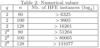
monomials. Thus the number of all HFE instances, i.e. quadratic polynomials which has more than two terms, linearly equivalent to some monomial is

n+1

2 |GLn(Fq)| − 1

2n(n+ 1)(q

n_{−1), forq >2,} n−1

2 |GLn(Fq)| − 1

2n(n−1)(q

n_{−1), forq= 2.}

Table 2 shows the numerical value of the above formula for some specific parameters. We can see that there are huge number of HFE instances linearly equivalent to some monomial.

Table 2: Numerical values q n Nb. of HFE instances (log2)

2 80 >6325 2 100 >9905 2 128 >16261 28 _{80 >51204}

28 _{100 >80005}

28 _{128 >131077}

In summary, the results of this section not only answer how many cryptographic schemes at most we can derive from monomials (Theorem 10) but also show that quite many HFE cryptosystems are equivalent to MI-type schemes (Theorem 14). However, it is not clear how to decide efficiently if a HFE scheme is equivalent to a MI-type scheme.

5. Conclusion and Future works

In this article, we brought a new question related to the IP problem, i.e. to determine the number of all the isomorphism equivalence classes of quadratic homogeneous poly-nomial systems. This question is related to equivalent keys and equivalent schemes of multivariate cryptography. By adopting a new tool of finite geometry, we have provided a framework for approaching to the question. Though determining all the equivalence classes is still an open problem, it seems that finite geometry is a good language to study it.

References

[1] Tsutomu Matsumoto and Hideki Imai. Public quadratic polynomial-tuples for efficient signature-verification and message-encryption. InAdvances in Cryptology – EUROCRYPT 1988, volume 330 ofLNCS, pages 419–453. Springer–Verlag, 1988.

[2] Jacques Patarin. The Oil and Vinegar signature scheme. presented at the Dagstuhl Workshop on Cryptography, 1997.

[3] Jacques Patarin, Louis Goubin, and Nicolas Courtois. C∗_{−+ and hm: Variations around two}