Research on Space-Time Adaptive Processing with Respect
to the Signal Powers
Wei Wang1, 2, *, Lin Zou1, and Xuegang Wang1
Abstract—Diverse array processing methods with higher order statistics (HOS) have been developed in the last three decades. One of the main interests in using HOS relies on the increase of effective aperture and the number of sensors of the considered array. In this work, we further exploit space-time adaptive processing (STAP) using HOS based on the phased array radar with uniform linear array (ULA). We implement STAP with respect to signal powers instead of with respect to signal amplitudes as the convention. The purpose of this paper is to provide some important insights into the STAP with respect to signal powers (SP-STAP), such as the output response, output signal-to-interference-plus-noise ratio (SINR), minimum detectable velocity (MDV) performance and effect of internal clutter motion (ICM). Compared with the conventional STAP under the condition of the same number of array elements and transmitting pulses, the simulation results show that SP-STAP can gain narrower target main beam, lower side-lobe levels, better MDV performance and less deleterious effect of ICM.
1. INTRODUCTION
Space-time adaptive processing (STAP) [1–4] is a crucial technique of clutter suppression and target detection for airborne/spaceborne moving target indicator (MTI) radar. It can adaptively adjust a two-dimensional space-time filter response to maximize the output signal-to-interference-plus-noise ratio (SINR), and thus provide a better target detection performance in strong clutter environments. The performance of STAP is relevant to the effective system degrees of freedom (DOFs). In particular, better minimum detectable velocity (MDV) performance can be obtained with more effective system DOFs. For instance, compared with the phased array radar, MIMO radar can achieve more effective system DOFs due to its orthogonal transmitting waveforms. However, the waveforms are generated by those extra waveform control modules at the expense of design and control complexities [5, 6]. Moreover, it is well known that a sparse array increases the virtual aperture dimension for a given physical aperture area, which can be regarded as effective system DOFs extension. (Virtual aperture dimension refers to the total length of the array from one end to the other, whereas, physical aperture area refers to the are a actually covered by aperture hardware.) [7]. A reference for an effective sparse array and the design procedure can be found in [8]. In comparison with the dense array, the sparse array can reduce the antenna pattern clutter Doppler spread and the Doppler width of blind zones, which results in better MDV performance [7, 9]. However, the sparse array causes grating lobes and may introduce additional Doppler blind zones in the case of high sparsity [7]. In practice, the phased array radar with uniform linear array (ULA) is widely used in the civil or military field. Though its system DOFs can be simply increased by adding the number of array elements or transmitting pulses, the equipment weight and size or the duration of coherent processing interval (CPI) will increase at the same time. However, the load of airborne/spaceborne platform is limited, and we commonly wish to decrease the weight or
Received 14 January 2018, Accepted 25 February 2018, Scheduled 21 March 2018 * Corresponding author: Wei Wang ([email protected]).
1 School of Electronic Engineering, University of Electronic Science and Technology of China, Chengdu, China.2China Aerodynamics
size as possible as we can. In addition, too long CPI duration will result in serious range-walk, which largely affects the STAP performance [2]. Therefore, we expect to increase the effective system DOFs without changing system hardware frame work or just increasing transmitting pulses for the purpose of saving hardware resource, reducing upgrade difficulty of hardware and avoiding some other performance declines.
On the other hand, for about three decades, higher order statistics (HOS) have been extensively used in many diverse application fields [10]. For example, many HOS-typed methods which make use of fourth order statistics of non-Gaussian signals have been developed for both direction finding [11, 12] and blind identification [13, 14]. Moreover, some other algorithms that exploit data statistics at an arbitrary even order have been developed in [15–18] for array processing. Note that those aforementioned HOS-typed methods can increase even more spatial resolution, robustness to modeling errors, and number of sources to be processed than traditional second-order statistics (SOS) methods based on an eigen structure [18]. This fact is reasonable when one considers that using SOS, commonly represented as a covariance matrix, is a data reduction technique [19]. According to information theory, it is well known that we always lose information by data reduction. Using HOS, which is usually represented as a cumulant matrix, can be considered as an alternate data reduction technique. However, it is a much better one since it is possible to recover more information from the cumulant matrix about the sources illuminating the array [19]. Additionally, the virtual array (VA) concept has been presented as a powerful tool for performance evaluation of HOS-typed array processing methods [19–21]. In summary, according to the information theory and VA concept, we can consider that one of the main reasons for the improvements of HOS-typed array processing methods relies on the increase of the effective aperture and the number of sensors of the considered array, i.e., the increase of effective system DOFs [21].
Recently, a nonlinear adaptive spatial beamforming technique using HOS performed on nested array has been described in [22]. This proposed scheme implemented beamforming with respect to signal powers instead of with respect to signal amplitudes as is the convention. This approach needs to take the autocorrelation of the received signal vector and enables us to perform beamforming with the full DOFs of the difference co-array and gain O(N2) DOFs using only N physical sensors. It can be regarded as a HOS-typed algorithm. Enlightened by [22], a novel nonlinear STAP method using HOS has been applied to nested array, but the performances of the new method have not been exhaustively discussed in [23].
In this work, we continue to exploit STAP using HOS and further study a novel HOS-typed STAP method, which is referred to as SP-STAP, based on the phased array radar with ULA. In this method, signal powers are taken as the inputs of the space-time filters for the purpose of obtaining more effective system DOFs without altering system hardware framework or adding transmitting pulses. The aim of this paper is to make some important investigations into SP-STAP, such as the output response, the output signal-to-interference-plus-noise ratio (SINR), the minimum detectable velocity (MDV) performance and the effect of internal clutter motion (ICM). Compared with the conventional STAP under the condition of the same number of array elements and transmitting pulses, the simulation results show that SP-STAP can get narrower target main beam, lower side-lobe levels, better MDV performance and less deleterious effect of ICM. The manuscript is organized as follows. The rationale of SP-STAP based on ULA is presented in Section 2. Comparative simulations and results are addressed in Section 3. Conclusions are finally summarized in Section 4.
2. RATIONALE OF SP-STAP BASED ON ULA
Consider aN elements ULA with inter-element spacingd=λ/2, whereλindicates the radar wavelength, and the spatial steering vector can be given by
a(fs) =
1, ej2πfs, . . . , ej2πfsn, . . . , ej2πfs(N−1)
T
(1)
wheren= 0,1, . . . , N−1, [·]T denotes the transpose operation, andf
s is the spatial frequency which is
given by
fs= d
sin(θ)
where θ is the angle of arrival (AOA). In addition, given M transmitting pulses with pulse repetition interval (PRI)T in a CPI for a fixed radar range bin, the Doppler steering vectorb(fd) can be written
as
b(fd) =
1, ej2πfd, . . . , ej2πfdm, . . . , ej2πfd(M−1)
T
(3)
wherem= 0,1, . . . , M −1 and fdis the normalized Doppler frequency which is given by
fd=
2vsin(θ)T
λ =βfs (4)
where β = 2vTd and v is the relative velocity between the moving radar platform and the signal source from direction θ. Note that to avoid temporal aliasing, T should be chosen such that−0.5≤fd≤0.5.
Then, the space-time steering vector vcan be expressed as
v=b(fd)⊗a(fs) (5)
where⊗ denotes the Kronecker product.
Suppose that a target is located at spatial frequency fst with normalized Doppler frequency fdt,
and the target signal s can be written as
s=αtb(fdt)⊗a(fst) =αtvt (6)
where αt is the complex target amplitude, and vt denotes the target space-time steering vector.
Remarkably, we mainly consider the clutter scenarios without jamming in this paper, and Nc clutter
patches are supposed to be uniformly distributed among the angle 0◦ to 360◦ for a fixed range bin. The whole clutter signals can be given by
c=
Nc
i=1
αib
fdci
⊗afsci
=
Nc
i=1
αivi= Nc
i=1
ci (7)
where αi, fsci , fdci , vi and ci denote the complex amplitude, spatial frequency, normalized Doppler
frequency, space-time steering vector and return signal of theith clutter patch, respectively. Accordingly, the received data snapshot x, which consists of target, clutter and noise, can be expressed by
x=s+c+n (8)
wheren denotes the noise vector.
It is assumed that the clutter patches are mutually uncorrelated, and then the clutter covariance matrix (CCM)Rc can be given by [2]
Rc = Nc
i=1
EcicHi
(9)
where [·]H is the conjugate transpose operation, andE[·] indicates the expectation operator. The noises are also assumed to be mutually uncorrelated, and then the noise covariance matrixRncan be described
as
Rn=σ2nIM N (10)
whereσ2n is the noise power, andIM N is an M N×M N identity matrix.
For the conventional STAP method, one tries to find a weight vector w for direct filtering the received data snapshotx. The filter output y can be obtained by
y=wHx. (11)
The output SINR can also be given by
SINR = w
Hs 2 wHR
Iw
(12)
where RI = Rc+Rn is the covariance matrix of the clutters plus noises in the assumption that the
clutters are independent of the noises. To achieve an upper bound of performance in the maximum SINR sense, the optimum space-time weight vector wopt can be given by [1]
whereκis an arbitrary scalar that does not alter the output SINR, andR−I1 denotes the inverse matrix of RI. Then the upper bound of SINR, which is called as the optimum SINR, can be given by [1]
SINRopt=sHR−I1s. (14)
Note that the conventional STAP method, which employs the covariance matrix of signal amplitudes to construct the filter weights and make them work on the received signal vector, is regarded as an SOS-type algorithm. Furthermore, in order to make use of more information contained in HOS, a new SP-STAP method takes signal powers as the inputs of the space-time filter. Then we will completely deduce the data model and the output SINR expression of SP-STAP in the follows.
Firstly, a new vectorz, which is named as power space-time steering vector, is defined by
z=v∗⊗v (15)
where [·]∗ denotes the conjugate operation. Accordingly, a new power vector of the target signal can be constructed as
sp = vecssH=σ2t(v∗t ⊗vt) =σt2zt (16)
where vec(·) denotes vectorization operation, zt the power space-time steering vector of target, and
σt2 = E[|αt|2] the target signal power. Similarly, a new power vector corresponding to Nc clutter
patches can also be written as
cp = vec (Rc) = Nc
i=1
σi2(v∗i ⊗vi) = Nc
i=1
σi2zi = Nc
i=1
cp,i (17)
whereσi2=E[|αi|2] denotes the power of theith clutter patch, andzi andcp,i are the power space-time
steering vector and power vector of the ith clutter patch. Thus, the clutter power covariance matrix (CPCM) can be obtained by
Rcp= Nc
i=1
Ecp,icHp,i
. (18)
Moreover, a new noise power vector is given by
np = vec (Rn) =σ2n1n (19)
where1n= [eT1,eT2, . . . ,eTM N]T and ej(j = 1, . . . , M N) is a column vector of all zeros except for a one in thejth position. Meanwhile, the new noise power covariance matrix can also be acquired by
Rnp =E
npnHp
. (20)
Consequently, the power snapshot of the received data for SP-STAP can be formulated as
xp=sp+cp+np. (21)
The SP-STAP filter output with respect to xp is certainly given by
yp =wHp xp (22)
where wp is a new weight vector corresponding to the signal powers. The corresponding output SINR can be computed by
SINRp =
wHp sp 2 wH
p RIpwp
(23)
whereRIp=Rcp+Rnp. Then, the expression (23) can achieve its upper bound whenwpis substituted by the optimum weight vectorwp-opt, which is given by
wp-opt=γR−Ip1sp (24)
whereγ is an arbitrary scalar which does not alter the output SINR, andR−Ip1 is the inverse matrix of
RIp. Then the optimum output SINR of SP-STAP can be given by
SINRp-opt=sHp R−Ip1sp. (25)
As is evident, SP-STAP depends on the new power vectors sp and cp, which are obtained by the
3. NUMERICAL SIMULATION
In this section, a set of comparative simulations between SP-STAP and the conventional STAP are carried out. The clairvoyant SINR-loss, which is generally defined by comparing the clutter-limited performance to the noise-limited capability, is employed as one of the primary evaluated criteria in this work. The clutter-limited performance is represented by the optimum SINR, while the noise-limited capability is represented by the signal-to-noise ratio (SNR). Then, the clairvoyant SINR-loss of the conventional STAP can be written by
SINRloss=
SINRopt
SNR =
sHR−I1s
M Nσ2t σn2
. (26)
On the other hand, the clairvoyant SINR-loss of the SP-STAP can be given by
SINRp-loss= SINRp-opt SNRp =
sHp R−Ip1sp
(M N)2σt4 σ4n
. (27)
In the next simulations, the number of array elements is N = 6, and the number of transmitting pulses in a CPI is M = 6. The carrier frequency is 10 GHz, and the pulse repetition frequency (PRF) is 600 Hz, i.e., T = 1/PRF. To avoid temporal aliasing, β is equivalent to 1. A hypothetic target is located at angle 33.5 degrees, and its normalized Doppler frequency is assumed to be−0.21. The noise power is normalized to 0 dB, and the clutter-to-noise ratio (CNR) is 40 dB for all clutter patches.
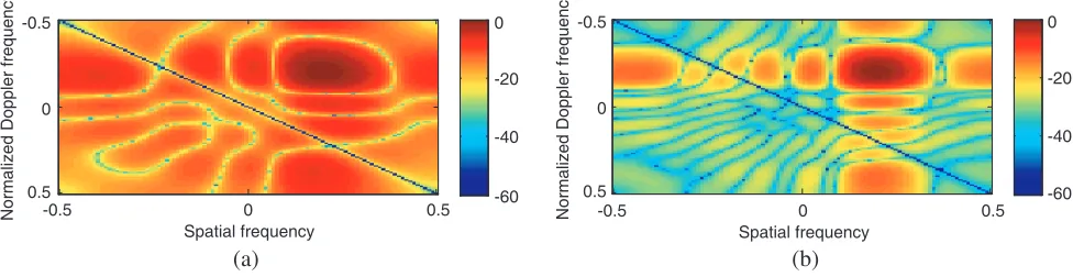
Figures 1(a) and 1(b) show the normalized space-time filter output responses of the conventional STAP and SP-STAP, respectively. It can be seen from the two pictures that both of the methods can form a deep notch at the clutter ridge and make a maximum peak at the target position. Nevertheless, the side-lobe levels of SP-STAP are lower than those of the conventional STAP. For the sake of explicit display, the spatial and normalized Doppler frequency principal plane cuts at the target location are illustrated in Figures 2(a) and 2(b), respectively. It is shown that the target main beam of SP-STAP is even narrower than that of the conventional STAP.
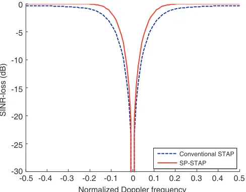
Next, fixing the angle atθ= 0◦ the clairvoyant SINR-loss curves of SP-STAP and the conventional STAP are shown in Figure 3, respectively. It is demonstrated that the clutter notch width of SP-STAP is smaller than that of the conventional STAP, which means that the MDV performance of SP-STAP is better than that of the conventional STAP. Therefore, SP-STAP has a greater potential to detect lower velocity target.
As aforementioned before, the SP-STAP method can increase effective system DOFs to improve the MDV performance without changing hardware architecture or adding transmitting pulses. To verify this standpoint strictly, we compare the SINR-loss of SP-STAP with that of the conventional STAP indifferent cases of array elements and transmitting pulses. The SINR-loss curve of SP-STAP with (N = 6, M = 6), and the SINR-loss curves of the conventional STAP with (N = 6, M = 6), (N = 7,
M = 7), (N = 8,M = 8) and (N = 9, M = 9) are all presented in Figure 4. Figure 4(b) is the closeup
(a) (b)
-0.5 0 0.5
Spatial frequency
-0.5 0 0.5
Spatial frequency -0.5
0
0.5
Normalized Doppler frequency
-0.5
0
0.5
Normalized Doppler frequency
0
-20
-40
-60
0
-20
-40
-60
(a) (b) -0.5
Spatial frequency
-0.4 -0.3 -0.2 -0.1 0 0.1 0.2 0.3 0.4 0.5 -0.5
Spatial frequency
-0.4 -0.3 -0.2 -0.1 0 0.1 0.2 0.3 0.4 0.5 0
10
-10
-20
-30
-40
-50
-60
Output (dB)
0 10
-10
-20
-30
-40
-50
-60
Output (dB)
conventional
SP-STAP
conventional
SP-STAP
Figure 2. Principal plane cuts at the target location. (a) Spatial cuts, (b) Doppler cuts.
-0.5 -0.4 -0.3 -0.2 -0.1 0 0.1 0.2 0.3 0.4 0.5 Normalized Doppler frequency
Conventional STAP SP-STAP
0
-5
-10
-15
-20
-25
-30
SINR-loss (dB)
Figure 3. The clairvoyant SINR-loss.
of Figure 4(a). It is well known that the apparent system DOFs of STAP can be represented by the number of array elements and transmitting pulses. Therefore, as shown in Figure 4, the clutter notch width of the conventional STAP decreases with the increase of array elements and transmitting pulses. In other words, the MDV performance improves with the increase of DOFs. On the other hand, we can see that the clutter notch width of SP-STAP with (N = 6,M = 6) is still smaller than that of the conventional STAP with (N = 6,M = 6). Meanwhile, it is almost the same as the clutter notch width of the conventional STAP with (N = 9, M = 9). The result can be owing to the increasing effective system DOFs caused by the HOS characteristics of the SP-STAP method. Consequently, it has been demonstrated again that the SP-STAP method is able to get higher effective system DOFs and better MDV performance than the conventional STAP method under the condition of the same number of array elements and transmitting pulses.
(a) (b) Normalized Doppler frequency
-0.5 -0.4 -0.3 -0.2 -0.1 0 0.1 0.2 0.3 0.4 0.5
Normalized Doppler frequency
-0.14 -0.12 -0.1 -0.08 -0.06 -0.04 -0.02 0 0
-5
-10
-15
-20
-25
-30
SINR-loss (dB)
0
-5
-10
-15
SINR-loss (dB)
N = 6, M = 6
N = 7, M = 7
N = 8, M = 8
N = 9, M = 9 SP N = 6, M = 6
N = 6, M = 6
N = 7, M = 7
N = 8, M = 8
N = 9, M = 9 SP N = 6, M = 6
Figure 4. The clairvoyant SINR-loss for different system DOFs. (a) Original curves, (b) close up of original curves.
-0.5 -0.4 -0.3 -0.2 -0.1 0 0.1 0.2 0.3 0.4 0.5 Normalized Doppler frequency
Conventional STAP SP-STAP
0
-5
-10
-15
-20
-25
-30
SINR-loss (dB)
Figure 5. The output SINR-loss with ICM.
4. CONCLUSION
REFERENCES
1. Melvin, W. L., “A stap overview,” IEEE Aerospace and Electronic Systems Magazine, Vol. 19, No. 1, 19–35, Jan. 2004.
2. Klemm, R., “Principles of space-time adaptive processing,” The Institution of Engineering and Technology, London, UK, 2006.
3. Guerci, J. R.,Space-time Adaptive Processing for Radar, Artech House, Boston, USA, 2003. 4. Li, X. M., D. Z. Feng, H. W. Liu, and D. Luo, “Dimension-reduced space-time adaptive clutter
suppression algorithm based on lower-rank approximation to weight matrix in airborne radar,”
IEEE Transactions on Aerospace and Electronic Systems, Vol. 50, No. 1, 53–69, Jan. 2014.
5. Liu, H. W., Y. S. Zhang, Y. D. Guo, et al., “A novel STAP algorithm for airborne MIMO radar based on temporally correlated multiple sparse Bayesian learning,” Mathematical Problems in Engineering, 2016.
6. Chen, C. Y. and P. P. Vaidyanathan, “MIMO radar space-time adaptive processing using prolate spheroidal wave functions,” IEEE Trans. Signal Process., Vol. 56, No. 2, 623–635, Feb. 2008. 7. Leatherwood, D. A., W. L. Melvin, and R. Acree, “Configuring a sparse aperture antenna for
spaceborne MTI radar,” IEEE Radar Conference, 139–146, Alabama, USA, May 2003.
8. Morabito, A. F., A. R. Lagana, and T. Isernia, “Isophoric array antennas with a low number of control points: A ‘size tapered’ solution,” Progress In Electromagnetics Research Letters, Vol. 36, 121–131, 2013.
9. Tang, B., X. Yang, H. Wu, and W. Peng, “Research on clutter spectra and STAP for sparse antenna arrays,” International Conference on Communications, Circuits and Systems (ICCCAS), Vol. 1, 280–283, Chengdu, China, Nov. 2013.
10. Mendel, J. M., “Tutorial on higher-order statistics (spectra) in signal processing and system theory: Theoretical results and some applications,” Proceedings of the IEEE, Vol. 79, No. 3, 278–305, Mar. 1991.
11. Cardoso, J. F. and E. Moulines, “Asymptotic performance analysis ofdirection finding algorithms based on fourth order cumulants,”IEEE Trans. Signal Process., Vol. 43, No. 1, 214–224, Jan. 1995. 12. G¨onen, E. and J. M. Mendel, “Applications of cumulants to array processing — Part VI: Polarization and direction of arrival estimation with minimally constrained arrays,” IEEE Trans. Signal Process., Vol. 47, No. 9, 2589–2592, Sep. 1999.
13. De Lathauwer, L., B. De Moor, and J. Vandewalle, “ICA techniques formore sources than sensors,”
Proc. Workshop Higher Order Statistics, Caesara, Israel, Jun. 1999.
14. Ferreol, A., L. Albera, and P. Chevalier, “Fourth order blind identification of under determined mixtures of sources (FOBIUM),” Proc. ICASSP, 41–44, Hong Kong, Apr. 2003.
15. Albera, L., A. Ferreol, P. Comon, and P. Chevalier, “Blind identification of overcomplete mixtures of sources (BIOME),”Linear Algebra and Its Applications, Vol. 391, 3–30, Nov. 2004.
16. Chevalier, P., A. Ferreol, and L. Albera, “High resolution direction finding from higher order statistics: The 2q-MUSIC algorithm,” IEEE Trans. Signal Process., Vol. 54, No. 8, 2986–2997, Aug. 2006.
17. Birot, G., L. Albera, and P. Chevalier, “Sequential high-resolution direction finding from higher order statistics,” IEEE Trans. Signal Process., Vol. 58, No. 8, 4144–4155, Aug. 2010.
18. Wang, F., X. Cui, and M. Lu, “Direction finding using higher order statistics without redundancy,”
IEEE Signal Processing Letters, Vol. 20, No. 5, 495–498, May 2013.
19. Dogan, M. C. and J. M. Mendel, “Applications of cumulants to array processing — Part I: Aperture extension and array calibration,”IEEE Trans. Signal Process., Vol. 43, No. 5, 1200–1216, May 1995. 20. Chevalier, P. and A. Ferreol, “On the virtual array concept for the fourthorder direction finding
problem,”IEEE Trans. Signal Process., Vol. 47, No. 9, 2592–2595, Sep. 1999.
22. Pal, P. and P. P. Vaidyanathan, “Nested arrays: A novel approach to array processing with enhanced degrees of freedom,” IEEE Trans. Signal Process., Vol. 58, No. 8, 4167–4181, Aug. 2010. 23. Vouras, P., “Fully adaptive space-time processing on nested arrays,” IEEE Radar Conference,
0858–0863, Virginia, USA, May 2015.