Scholarship@Western
Scholarship@Western
Electronic Thesis and Dissertation Repository
4-24-2018 1:30 PM
Simplified Numerical Models in Simulating Corona Discharge and
Simplified Numerical Models in Simulating Corona Discharge and
EHD Flows
EHD Flows
Sara Mantach
The University of Western Ontario
Supervisor
Adamiak, Kazimierz
The University of Western Ontario
Graduate Program in Electrical and Computer Engineering
A thesis submitted in partial fulfillment of the requirements for the degree in Master of Engineering Science
© Sara Mantach 2018
Follow this and additional works at: https://ir.lib.uwo.ca/etd
Part of the Electromagnetics and Photonics Commons
Recommended Citation Recommended Citation
Mantach, Sara, "Simplified Numerical Models in Simulating Corona Discharge and EHD Flows" (2018). Electronic Thesis and Dissertation Repository. 5357.
https://ir.lib.uwo.ca/etd/5357
This Dissertation/Thesis is brought to you for free and open access by Scholarship@Western. It has been accepted for inclusion in Electronic Thesis and Dissertation Repository by an authorized administrator of
Corona discharge is used in many practical applications. For designing and optimization of corona devices, the discharge phenomenon should be numerically simulated. Most often, the corona discharge model is simplified by neglecting the process dynamics and assuming a limited number of reactions and species. In the extreme case, monopolar corona models with just one species and no reactions are studied. However, there is a problem with determining boundary conditions for the space charge density. The simplest solution to this problem was suggested by Kaptzov, who hypothesized that the electric field on the electrode surface remains constant and equal to the value at the onset conditions, which is known from a semi-empirical Peek’s formula. Experimental data confirm good accuracy of this approach. However, it is impossible to experimentally measure the surface electric field at different voltage levels and compare it to Peek’s value. Our thesis will discuss different methods for simulating corona discharge in 1D wire-cylinder geometry in air at atmospheric pressure. The classical model based on Kaptzov’s hypothesis is compared with other approaches. The first model is still a single-species one, but it uses direct ionization criterion. Two other models consider a higher number of species and some number of reactions, so the ionization layer is included. The surface electric field can differ from Peek’s value by almost 43%. In addition, the results of numerical investigations of the EHD flow generated by dc corona discharge in the point-plane configuration in atmospheric air are presented in this thesis. A computational model of the discharge includes the ionization layer and three ionic species. The most important ionic reactions (ionization, attachment, recombination and detachment) are considered. The results of the corona simulations were used to predict the secondary EHD flow. All flow parameters (velocity components, pressure, streamlines) are determined. In addition to main flow vortex reported before, a local vortex near the discharge tip has also been discovered. COMSOL, a commercial finite element package, was used in simulations.
Keywords
ii
Dedication
iii
Acknowledgments
I am very grateful for my supervisor Prof. Kazimierz Adamiak. Your invaluable help, constant support and clear guidance throughout my research program were truly a blessing. Thank you for your patience and kindness. I really appreciate the chance you offered me to be a part of your research team.
iv
Table of Contents
Abstract ... i
Dedication ...ii
Acknowledgments ... iii
Table of Contents ... iv
List of Tables ... vii
List of Figures ...viii
Chapter 1 ... 1
1 Introduction ... 1
1.1 Introduction ... 1
1.2 Thesis Objectives ... 2
1.3 Thesis Outline ... 3
Chapter 2 ... 5
2 Literature review ... 5
2.1 Early Discovery of Corona Discharge ... 5
2.2 Numerical Simulation of Corona Discharge ... 6
2.2.1 Numerical Techniques to Calculate the Electrical Field ... 7
2.2.2 Numerical Techniques to Calculate the Space Charge Density ... 8
2.2.3 Numerical Investigation of Corona Discharge ... 9
2.3 Electrohydrodynamic Flow ... 12
Chapter 3 ... 15
3 Mathematical Model and Numerical Algorithm for Simulating Corona Discharge .... 15
3.1 Single-Species Approach ... 15
3.1.1 Idealizing Assumptions ... 15
v
3.2 Three-Species Approach ... 19
3.2.1 Governing Equations ... 19
3.3 Seven-Species Approach ... 21
3.3.1 Governing Equations ... 21
3.4 Numerical Algorithm ... 23
3.4.1 Numerical Algorithm for Single-Species Models ... 23
3.4.2 Numerical Algorithm for Multispecies Models ... 24
3.5 Governing Equation for the EHD Flow ... 25
3.6 Conclusions ... 26
Chapter 4 ... 27
4 Validation of Kaptzov’s Hypothesis for Wire-Cylinder Configuration in Air ... 27
4.1 Description of the Model ... 27
4.2 Single-Species Model ... 27
4.3 Three-Species Model ... 31
4.4 Seven-Species Model ... 34
4.5 Electric Field at the Corona Wire ... 39
4.6 V-I Characteristic Curves ... 40
4.7 Conclusions ... 42
Chapter 5 ... 43
5 Electrohydrodynamic Flow ... 43
5.1 Model Description ... 43
5.1.1 Geometry ... 43
5.1.2 Discretization ... 43
5.1.3 Corona and Flow Model ... 45
5.2 Simulation Results ... 45
vi
5.4 Conclusions ... 63
Chapter 6 ... 64
6 Conclusions ... 64
6.1 Summary of the Thesis ... 64
6.2 Unsuccessful Attempts with Corona Simulation ... 65
References ... 67
vii
List of Tables
Table 3-1: Swarm parameters for the ionic reactions in oxygen ... 20
viii
List of Figures
Figure 4-1: Electric field in the air gap between electrodes at three different voltage levels for
the single species models ... 29
Figure 4-2: Space charge density distribution at three different voltage levels for the single species models... 30
Figure 4-3: Total number of negative ions for different voltage levels from the model using Kaptzov’s hypothesis and the direct ionization criterion. ... 30
Figure 4-4: Ionic species distribution for voltage levels of -7.3 kV and -12 kV ... 34
Figure 4-5: Ionic species distribution of seven-species model for voltages -7.3 kV and -12 kV ... 38
Figure 4-6: Electric field on the corona wire for the four investigated models ... 39
Figure 4-7: V-I curve for the four investigated models... 41
Figure 5-1: Discretization of the computational domain ... 44
Figure 5-2: V-I characteristic curve ... 45
Figure 5-3: Validation of Peek's formula in point-plane configuration ... 46
Figure 5-4: Electric field distribution near the needle surface... 47
Figure 5-5: Distribution of all ionic species in the air gap for voltages -8 kV and -12kV ... 50
Figure 5-6: Variation of number of different ionic species with voltage ... 51
Figure 5-7: Spatial distribution of body force near the needle tip ... 53
Figure 5-8: Axial component of the EHD body force along the axis of symmetry ... 54
ix
Figure 5-10: Velocity magnitude of the airflow at -8 kV and -12 kV ... 58
Figure 5-11: Axial flow velocity ... 60
Figure 5-12: Axial velocity along axis of symmetry for different voltage levels ... 61
Figure 5-13: Maximum and minimum axial velocities for different voltage levels ... 62
Chapter 1
1
Introduction
An introduction to the corona discharge phenomenon, thesis objectives and thesis outline are presented in this Chapter.
1.1
Introduction
In a non-uniform configuration consisting of two or more electrodes, a stable electric discharge, called corona discharge, is produced when a sharp electrode is connected to a high voltage source. The other, much flatter, electrode is usually connected to ground. Because of the difference in the radii of curvature of both electrodes, a high field region is produced near the sharp electrode. If there is an electron in this region, it is accelerated and after reaching sufficient energy it can collide with a neutral molecule detaching another electron, so gas ionization takes place [1]. Positive ions and electrons are produced, and their movement depends on the polarity of the sharp electrode. When electrons leave the high field region, they don’t have enough energy to further ionize neutral molecules. In some gases, called electronegative ones, electrons attach to neutral molecules, forming negative ions. Therefore, two regions can be identified in the air gap between both electrodes: a lower field drift region and a high field ionization region [2]. Drift of ions and electrons leads to imposing some momentum on the neutral gas
molecules of the host medium, which causes the ionic wind, also known as electrohydrodynamic (EHD) flow.
The major published works on corona discharge may be credited to Loeb, Goldman and Sigmond [2,4]. Loeb analyzed the mechanism of negative corona pulses in air at
atmospheric pressure and studied the differences between positive and negative corona currents in air [4]. Robinson was the first to report the existence of ionic wind [5], but Chattok introduced its first quantitative analysis [6]. The lack of complete understanding of the physical processes taking place in corona discharge and important practical
applications of this phenomenon make the interest in corona discharge still alive today.
There are many practical applications of corona discharge in industry and research. Some of them are: charging thin insulating films, electrophotography, electrostatic
precipitation, removal of gaseous pollutants (mostly NOx and SOx) and many others. The
electrostatic precipitator was probably the first commercial application of the corona discharge phenomenon and this didn’t happen until 1907 [8]. On the other side, corona discharge is harmful in the electrical power systems, where it should be prevented since it causes power loss, produces audible noise and leads to radio interferences [9].
Corona discharge is a complex phenomenon and its experimental investigation is time consuming. Therefore, numerical simulation has been used more and more often. However, due to process complexity some simplifying assumptions are necessary. Despite this, relatively accurate solutions can be still obtained.
1.2
Thesis Objectives
The first objective of this thesis is to perform a numerical investigation of the negative DC corona discharge in atmospheric air in the wire-cylinder configuration. This investigation is done using three different approaches. The first approach includes one ionic species, where two numerical models are tested: one is based on Kaptzov’s
hypothesis and the other on the direct ionization criterion. The second approach includes three ionic species: electrons, negative ions and positive ions. The final approach in addition to the previous three species includes extra four species: O, O-, O
3 and O2(1∇g).
assumption, called Kaptzov’s hypothesis, can be validated, spatial distribution of electric charge and the current-voltage characteristics.
The second investigated geometry consists of a needle acting as the corona electrode which is perpendicular to a grounded plate. In this model, three ionic species are considered: electrons, positive ions and negative ions. The objective is to investigate a new air flow pattern that has not been reported before in literature on EHD.
To achieve both objectives, the numerical algorithm based on the Finite Element Method was implemented using commercial software COMSOL 5.3. As a result, the distributions of both space charge densities and electric potential can be determined.
Several data sets are reported, including the distribution of electric field on the corona electrode, the spatial distribution of the ionic species and the voltage-current
characteristics. In addition to this, three more parameters of interest are presented for the EHD flow. These include the airflow streamlines, the pressure distribution near the corona electrode, and the velocity distribution in the air gap between both electrodes.
1.3
Thesis Outline
The thesis is divided into 6 Chapters. The summary of each Chapter is as follows:
Chapter 2 includes a summary of some of the previous publications related to numerical simulation of negative corona discharge in wire-cylinder and needle-plate configuration in atmospheric air. Moreover, a review is done on the recent work related to
electrohydrodynamic flows. The review covers simulations of one-species, three-species and seven-species corona models. Moreover, the Kaptzov hypothesis and direct
ionization criterion are reviewed as well.
electric field and drift-diffusion for the charge transport are presented. In addition, the boundary conditions for all distributions are specified.
Chapter 4 includes the numerical investigation of the DC corona discharge in the wire-cylinder geometry. The electric field and space charge distributions are compared for different numerical models. The validity of Kaptzov’s hypothesis is verified.
Chapter 5 includes the simulation results of electrohydrodynamic flow in the point-plane geometry. The three-species model of the corona discharge is investigated first for the stationary discharge model. Determined electric field and space charge density are used to calculate the flow body force. The obtained results predict a double-vortex pattern never reported previously.
Chapter 2
2
Literature review
In this Chapter, a comprehensive literature review is presented regarding the theory and numerical simulation of DC corona discharge and electrohydrodynamic (EHD) flow. This review focuses on two configurations of electrodes: wire-cylinder and needle-plate. Various numerical approaches, from very simplistic to the most advanced are discussed.
2.1
Early Discovery of Corona Discharge
Peek was the first researcher to talk about the appearance of the corona in his book, which he published in 1929 [11]. He discovered that when the voltage between two smooth conductors increases above a certain critical potential, a hissing noise can be heard, a violet light can be observed, if the surrounding medium is dark, and a noticeable reading on a wattmeter is recorded. Peek also noticed the formation of ozone in this process. Moreover, when the air was electrically overstressed, the air constituents, oxygen O2 and nitrogen N2, chemically react, leading to the formation of oxides. As a
result, the corona discharge is accompanied by the power loss, which has several forms: chemical reactions, noise, light and heat. Peek also reported that the power loss recorded by a wattmeter increases significantly with the increase of the voltage level and also observed the difference between AC and DC corona discharge. The appearance of the AC corona for the positive half-cycle of the supplied voltage is the same as that of the
positive DC corona and the same applies to the negative corona. On the other hand, Peek discovered, using a stroboscope, the difference in the discharge pattern in the positive and negative corona discharges. In the case of the negative applied voltage, some reddish beads are formed on the wire. In the case of positive applied voltage, a smoother bluish-white glow is visible.
Any geometry that possesses a non-uniform gap can be used for generation of the corona discharge phenomenon. However, in practical situations geometries which have
electrodes with significantly different sharpness are more practical. The most commonly studied systems have been the point-to-plane, where the point can be a tip of sharp needle, and the coaxial wire-cylinder systems. In 1965, Loeb explained the difference in the corona pattern between these two systems [12]. While the point-plane geometry has a confined discharge region, in the coaxial geometry the discharge can be initiated at different points on the corona wire.
2.2
Numerical Simulation of Corona Discharge
Numerous electrical, mechanical and chemical processes are associated with the electric corona discharge. To study this phenomenon, major simplifications should be
implemented. Even with such simplifications, analytical solutions can’t be obtained unless the geometry of the targeted physical problem is one-dimensional. As a result, since the 1960s numerical simulation of corona discharge has been of wide interest to researchers to enhance understanding of industrial and research processes [13]. The two major parameters involved in the simulation of corona discharge are the electric field and the space charge density. These quantities enable the calculation of the electric current, which is in turn the main factor needed for calculation of the power and energy loss. The electric field depends on the space charge magnitude and distribution and the space charge is affected by the electric-field distribution. As a result, both quantities are mutually coupled.
2.2.1
Numerical Techniques to Calculate the Electrical Field
The Poisson equation, which governs the electric potential distribution, is a linear partial differential equation of the second order. The techniques for solving this equation can be divided into two groups: differential and integral. The integral methods require the discretization of the active parts of the domain only, which are the electrode surfaces and areas with electric charge. The first integral technique is the Charge Simulation Method (CSM). In this technique, all electrodes are substituted with some number of lumped charges placed inside of the conducting objects. The magnitude of these charges is determined from the condition that the electrode surface should be equipotential. After that, the electric field is calculated by the superposition of the individual electric fields resulting from each point charge. This technique can’t be used for nonlinear problems, or for systems having complex geometries, or for infinite electrodes [15].
The second technique uses a similar philosophy and is called the Boundary Element Method (BEM). The unknown in this technique is the surface charge density on the electrode surface, which is determined from the condition of electrode equipotential. These charges physically exist, so the method doesn’t rely on artificial charges used in CSM. Mathematically, the method is based on solving integral equations with weakly singular kernels, which makes the approach more complicated. While solution of the Laplace equation (problems without space charge) is relatively fast, problems with space charge are much more time consuming [16].
On the other hand, the differential methods require the discretization of the whole computational domain, which causes problems for open physical problems. The
matrix equations for each element, assembling the element equations and, finally, solving the obtained system of equations where the solution over each element is interpolated using a simple function, most often polynomials. A fine discretization of the domain may lead to large algebraic systems. This technique is easily used to solve problems with complex geometries [18].
2.2.2
Numerical Techniques to Calculate the Space Charge
Density
The knowledge of the electric field distribution in a given domain is needed to evaluate the space charge density. One of the most efficient techniques for this purpose is the Method of Characteristic (MOC), where the partial differential equations along the lines, along which the ions move, are reduced to the ordinary differential equations [18]. These lines are called characteristic lines. For single species models these equations have simple analytical solutions. Since it is more difficult to solve a set of ordinary differential
equations, application of this technique to the multiple species problems is more problematic.
Another technique, which can be used for the charge transport equations, is the Finite Volume Method (FVM); one of its versions is called the Donor-Cell Method (DCM) [19]. In this method, the domain is tessellated by closed polygonal paths and each
polygon has a node enclosed in it. DCM is based on the integral form of the conservation of charges, where each polygon bounds points that are nearer to the node inside the polygon than any other node. This technique can handle problems with multiple species; however, it is time consuming [20].
where the physical diffusion coefficient used in the drift-diffusion equations is modified according to the following equation:
D#$%&'(')*+ = D-./#'0%(+ δh|v| ( 2-1)
where 𝛿 is a stabilizing parameter between 0 and 0.5, h is the longest mesh side element and v is the charged species drift velocity. The drawback of such technique is that it adds artificial diffusion in all directions; thus, making it an inconsistent method. The other two consistent methods are the streamline diffusion and crosswind stabilization. Streamline diffusion adds the artificial terms in the direction of the electric field only [7]. This technique is considered consistent because the stabilizing term tends to zero when the solution converges. In the crosswind stabilization an artificial diffusion perpendicular to the electric field lines is added [37]. This technique is used for simulating models which have high electric fields.
Other methods are the Flux Corrected Transport (FCT) and the Total Variation Diminishing technique (TVD). FCT identifies the steep density gradient without introducing any artificial diffusion [63]. It adds an anti-diffusive term to the low-order solution making sure that no new maxima or minima associated with the new added terms are introduced. TVD on the other hand makes sure to eliminate any numerical oscillations which can result from the increase in the flow variables with time. As a result, although the solution can be of the second or third order in the smooth part, it changes to a first order at points where the artificial minima or maxima are generated.
2.2.3
Numerical Investigation of Corona Discharge
Each of the methods mentioned in the previous two sections has some advantages and disadvantages, where each is better for specific applications depending on the problem requirements. In order to handle simulations most efficiently, a combination of numerical methods should be considered, which leads to the idea of hybrid techniques.
three drift-diffusion equations for ionic species and the FDM method for solving
Poisson’s equation to determine electric field. A one-dimensional model was considered in this study.
The first published work, which reported using FEM only to simulate corona discharge was authored by Janischewskyj and Gela [18]. They simulated corona in a wire-cylinder configuration assuming a one-dimensional unipolar corona model. Deutsch assumption was satisfied in this simulation since the electrical field is always radial in this
configuration [22]. This assumption states that the intensity of the Laplacian field lines changes in the presence of space charge, but the geometry of the lines is preserved.
Abdel-Salam et al. used a hybrid FEM-CSM technique, for simulating corona discharge in wire-to-ground configuration [23, 24]. A monopolar corona model was used where the ionization layer was neglected. They assumed that the electrical field intensity on the corona wire is constant; thus, implementing Kaptzov’s hypothesis. Kaptzov’s hypothesis states that the electric field on the corona electrode is constant when the applied voltage is above a threshold value, called onset voltage. Chen and Davidson simulated positive and negative corona discharges in a wire-cylinder configuration [25]. A one- dimensional stationary model was adopted, where three ionic species (electrons, negative ions and positive ions) were taken into consideration. FDM was implemented to solve the charge continuity equations and Kaptzov’s hypothesis was adopted in this simulation.
Accurate results were attained when very fine discretization was used near the corona electrode, since the electric field has a very steep gradient in this area.
Some researchers studied the electric corona discharge using time-dependent and multi-polar models [28]. Liang et al. used a one-dimensional single species model in order to simulate a wire-cylinder electrostatic precipitator under the pulse energization [29]. Rajanikanth and Prabhakar used a two-dimensional single species model to simulate the same problem using a dependent model [30]. Salasoo and Nelson used a time-dependent two-dimensional multi-species model in order to simulate a pipe-type precipitator [31].
Many authors investigated negative and positive corona discharge in oxygen, air, SF6 and
other gases taking into consideration more detailed chemistry of ionic reactions.
Georghiou et al. simulated corona discharge in a point-plane geometry at radio frequency in air [28]. Detailed models were investigated considering multi-species and taking several ionic processes into account: the ionization of neutral molecules, attachment of electrons, the recombination between negative ions and positive ions and the
recombination between electrons and positive ions. Zhang and Adamiak used a similar approach to simulate corona discharge in oxygen in a point-plane geometry, where a DC stationary model was assumed [32].
Yanallah and Pontiga proposed a semi-analytical stationary discharge model in a point-plane configuration for both positive and negative corona discharge in oxygen. The approximate analytical expressions for the electric field and the ionic densities were found by solving the Gauss and the continuity equations. Secondary ionization criterion and photoionization were implemented in the boundary conditions of the problem by using the experimental corona current and applied voltage as inputs [33].
For the cylinder-wire-plate configuration, Dumitran et al. introduced a more realistic non-uniform charge injection that accounts for the field variation on the surface of the
In 2005, Adamiak et al. came up with a novel approach based on the direct ionization criterion instead of Kaptzov’s hypothesis and applied it for a two-dimensional hyperbolic needle-ground configuration. The new approach was compared with two others: one based on Kaptzov’s hypothesis and the other one based on the analytical Peek formula with an equivalent electrode radius [60]. BEM, FEM and MOC were combined to solve for the Laplacian electric field, the Poisson component of the electric field and the charge transport equation, respectively. The discharge current was practically the same for the three approaches However, the electric field distributions on the corona electrode surface were slightly different.
2.3
Electrohydrodynamic Flow
Electrohydrodynamic flow (EHD) is the result of the collisions between charged
particles, accelerated in the electric field, and neutral gas molecules. This leads to the rise of induced air flow, which has been called the “ion wind”.
EHD flow was first observed in 1629 by Cabeo, but the first official acknowledgement was reported in 1709 by Hauksbee [36,37]. Hauksbee discovered that a weak blowing wind is initiated near an electrified body [38]. Cavalo, in turn, provided the first qualitative explanation of the ionic wind [39]. Faraday identified the mechanism responsible for the movement of the air particles between two electrodes, when high voltage is applied to the emitter. He confirmed that ionic wind is driven by the momentum transfer between charged and uncharged particles [40]. In 1873, Maxwell published the most comprehensive work at that time, which is still valid nowadays [41].
The effect of many factors, including the electrodes geometry, the EHD force and the current-voltage characteristics on the velocity of the ionic wind has been studied. Zhao and Adamiak presented numerical investigation of the EHD flow produced by corona discharge [70]. Three different system configurations were considered with variable applied pressure. The development of the EHD flow to its full pattern has been investigated including the time it takes and the factors that affect it. Improved models were simulated including a set of continuity equations for the charged particles coupled with Poisson’s equation [75], where the corona model predicts the distribution of the EHD force and the flow velocity can be then obtained. A fully coupled model including both the continuity equations and the Navier-Stokes equations was proposed by Bérard et al [45]. The numerical investigation involved a steady state simulation of a 2D numerical model.
Some researchers tried to increase the gas flow velocity in a wire-plate configuration without reaching breakdown [56]. In 2014, an empirical model has been proposed linking the ionic wind velocity to the applied voltage and the geometry of the collecting electrode [57]. The measurements of the ions velocity and the discharge current were carried out for different electrode geometries, having a variable air gap length and applied voltage.
Chen et al. have reported the numerical and experimental study of a DC negative corona discharge in a needle-cylinder configuration [54]. They found that the gas near the needle tip flows towards the discharge electrode, while the gas velocity is oriented towards the ground electrode outside the ionization region. Moreover, the EHD force is
approximately two orders of magnitude higher in the ionization region than in the drift region.
classical plate discharge electrode [48]. Another configuration is a needle-ring-metal pump. In this configuration, the voltage is applied to both the needle and the ring. As a result, a higher flow velocity is observed [42]. A way to increase the flow velocity is to increase the active area of the pump. This is done by using a serial-staged configuration where a needle array is used [43].
The second application of EHD flow is the boundary layer control. The gas flow produced by the corona discharge is used to change the laminar-turbulent transition regime around obstacles [55]. This is done by changing the velocity in the layer that is very close to the surface of the object. Colver et al. performed a couple of numerical studies on the boundary layer control [73]. One significant aspect is the ion removal and deposition on the plate surface which have a small conductivity. The studies were performed using the Finite Difference Method and a coarse discretization was
implemented. Ghazanchaei proposed a model to numerically investigate the electrical and mechanical properties of a unipolar positive corona system around a flat plate by using FEM. He found that the efficiency of the system decreases at higher voltages and that the drag reduction occurs at higher velocities [55].
Chapter 3
3
Mathematical Model and Numerical Algorithm for
Simulating Corona Discharge
The corona systems investigated in this thesis consist of two electrodes, one having a much smaller radius of curvature then the other. The system investigated in Chapter 4 is a wire-cylinder configuration and in Chapter 5 it is a needle-plane configuration. In this Chapter, different discharge models are compared and they vary from a single-species to multi-species ones. In the most advanced approach, seven ionic species are considered with electron attachment, avalanche ionization and ionic recombination included. All these models will be used for 1D simulation, while the 2D discharge model is based on the three-species approach only. COMSOL, a commercial finite element package, is used for solving Poisson’s equation, governing the electric field distribution, in addition to convection-diffusion equations for all ionic species.
3.1
Single-Species Approach
3.1.1
Idealizing Assumptions
The essential processes in corona discharge are impact ionization of neutral molecules by electrons, attachment of electrons to neutral molecules, recombination of positive and negative ions, and others. The collision of accelerated electrons with gas molecules in the region with strong electric field leads to gas ionization and this takes place near the corona electrode. On the other hand, the presence of electrons in the region where the electric field is low leads to the attachment of these electrons to the neutral gas
electrode and its distribution is predicted by solving the coupled equations of the electric field and the charge transport.
3.1.2
Governing Equations
The first model considers the presence of just one ionic species. This is computationally less expensive than for other models, which consider the presence of three or more ionic species. The Poisson equation for the electric scalar potential is:
∇8V = −ρ
ε ( 3-1)
where ε is the permittivity of gas and ρ is the space charge density. The value of the space charge density ρis calculated by solving the charge transport equation.
In general case, the movement and generation of the ionic species are governed by the following drift-diffusion equation:
∇ ( − µ E@@⃗n − D∇n) = R ( 3-2)
where n is the species density (1/m3), D is the diffusion coefficient (m2/s), µ is the ion
mobility (m2/V·s ), R is the source term( 1/m3·s), and E is the electric field (V/m).
Since only one ionic species is considered in this model and no ion dissociation and recombination are considered, the source term is equal to zero. The relation between the space charge density ρ and density n is:
ρ = e · n ( 3-3)
where e is the electron charge equal to 1.602·10-19 C.
To solve the above equations, appropriate boundary conditions must be formulated. The corona and ground electrodes satisfy Dirichlet boundary conditions for the electric potential:
V= Vc on the corona electrode.
Two boundary conditions are also needed for the charge continuity equation. The first condition is a Neumann condition, where the normal derivative of the space charge density on the collecting electrode is zero. In addition to that, one boundary condition is needed for the space charge density on the corona electrode. Since ionization processes are ignored, the precise value of the space charge density can’t be determined. Two criterions were adopted for the boundary condition regarding the space charge density on the corona electrode: Kaptzov hypothesis and direct ionization criterion.
Moreover, in the 2D models, the computational domain is unlimited. In numerical algorithms this domain should be truncated by adding some artificial boundaries. The boundary conditions imposed on these artificial boundaries are: zero charge for the electrostatic potential and zero flux for the charge transport [2]. It is also important that the artificial boundaries should be far enough from the needle tip, so that they wouldn’t affect the results.
3.1.2.1
Kaptzov’s Hypothesis
According to this hypothesis, at voltages above the onset level, the electric field on the corona electrode remains constant regardless of the voltage level [2]. The electric field for the wire-cylinder configuration in atmospheric air can be calculated from Peek’s formula:
E- = 3.1 · 10K L1 +0.308
√r P
( 3-4)
where r is the radius of the corona electrode in centimeters, and Ep is the Peek’s value in
V/m.
For the point-sphere configuration, a different version of Peek’s formula should be used:
E- = 3.1 · 10K L1 +
0.308 √0.5 r P
The same formula is commonly used for 2D cases, where the electrode radius is replaced with the sum of principal radii of curvature.
When the electric field is larger than Peek’s value, the space charge density should be increased until the electric field is close to this value. On the other hand, when the electric field is smaller than this value, a zero space charge density is assumed on the corona electrode [63].
3.1.2.2
Direct Ionization Criterion
When a free electron, having a sufficiently high energy, hits a neutral gas molecule, a new electron and a positive ion are produced according to the following equation:
e + A à e + AS + e ( 3-6)
where A is the atom, A+ is the positive ion and e is the electron.
This process is called ionization by collision or electron avalanche. If an electric field is applied between two parallel electrodes, electrons are accelerated while traveling from the cathode to the anode due to an action of the electric force. Ionization takes place, if the electron energy is higher than the ionization potential, which is energy needed to dislodge an electron from its atomic shell [58]. If one electron collides with neutral molecules α times per one of centimeter travel and if the initial number of electrons at the cathode is n0, then the number of the electrons reaching the anode is equal to:
N = nU exp (α d) ( 3-7)
where d is the distance between the cathode and the anode andα is called the Townsend’s first ionization coefficient.
This process of avalanche ionization would die after some time, because all electrons would be removed from the air gap. A sustained discharge requires new seed electrons generated by other mechanisms. Two the most important are photoionization and
radiation is propagated in all direction and is not affected by the electric field, so photoionization can generate ions at points of higher electric potential (in some sense it travels against electric field) and this can lead to sustained discharge.
On the other hand, secondary ionization is a process of ejecting electrons from the discharge electrode. The positive ions produced by the avalanche ionization are attracted towards the cathode electrode. If the energy of the positive ion is greater than double the cathodic metal work function, one electron is released to gas and a second electron neutralizes the positive ion. The released electrons are called secondary electrons and they are the source electrons for the next avalanches. The probability of this process is associated with Townsend’s secondary ionization coefficient γ. Like α, γ is the net
number of secondary electrons produced by one positive ion and its value depends on the gas pressure, ion velocity and the material of the electrode.
3.2
Three-Species Approach
3.2.1
Governing Equations
This model takes into consideration four chemical reactions including the electron avalanche ionization, the ionic recombination of the electrons and the positive ions, recombination of the positive and negative ions, and the electron attachment to neutral molecules [8]:
e + O8à 2e + 𝑂8S ( 3-8)
e + 𝑂8S( 𝑁
8S) à O8(N8) ( 3-9)
𝑂8^+ 𝑁
8S+ O8(N8) à N8+ O8+ O8(N8) ( 3-10)
e + O8à 𝑂8^ ( 3-11)
fourth equation is Poisson’s equation, which is used to calculate the electric potential distribution:
∇ ( − µ_ E@@⃗n_ – D_∇n_) = R_ ( 3-12)
∇ ( µa E@@⃗na – Da∇na) = Ra ( 3-13)
∇ ( − µb E@@⃗nb – Db∇nb) = Rb ( 3-14)
∇8V = −e(na− n_− nb) ε
( 3-15)
where ne , np , nn are the densities (1/m3) of electrons, positive ions and negative ions,
respectively, De, Dp, Dn are the diffusion coefficients (m2/s), µe , µp , µn are the mobilities
(m2/V·s), Re , Rp , Rn are the source terms( 1/m3·s), and E is the electric field (V/m). The
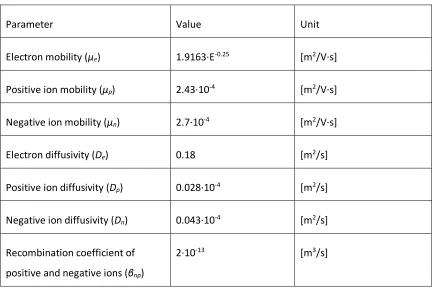
values of these parameters have been determined experimentally and are given in Table 3-1 [66].
Table 3-1: Swarm parameters for the ionic reactions in oxygen
Parameter Value Unit
Electron mobility (μe) 1.9163·E-0.25 [m2/V·s]
Positive ion mobility (μp) 2.43·10-4 [m2/V·s]
Negative ion mobility (μn) 2.7·10-4 [m2/V·s]
Electron diffusivity (De) 0.18 [m2/s]
Positive ion diffusivity (Dp) 0.028·10-4 [m2/s]
Negative ion diffusivity (Dn) 0.043·10-4 [m2/s]
Recombination coefficient of positive and negative ions (βnp)
Recombination coefficient of electrons and positive ions (βep)
2·10-13 [m3/s]
Ionization coefficient (α) 3.5·105·exp(-1.65·107/E) [1/m]
Attachment coefficient (η) 1.5·103·exp(-2.5·106/E) [1/m]
As seen in Table 3-1, the ionization reaction rate coefficients are expressed by using the local electrical field approximation. The following terms represent the reaction rates in equations for electrons, positive ions and negative ions:
R_ = α n_ µ_ E@@⃗ – η n_ µ_ E@@⃗ – β_a n_ na ( 3-16)
Ra = α n_ µ_ E@@⃗ – β_a n_ na ( 3-17)
Rb = η n_ µ_ E@@⃗ – βba nb na ( 3-18)
In order to have a self-sustained corona discharge model, some mechanism for generating seed electrons must be implemented. The most important source of these electrons is the secondary emission from the discharge electrode. When the positive ions collide with the negative corona electrode, the secondary electrons are ejected. The concentration of the secondary electrons is given by the following equation [72]:
n_ = γ · na· µa
µ_ ( 3-19)
where 𝑛* is the concentration of the electrons on the corona wire (1/m3). The secondary
emission coefficient γ is taken to be 0.001.
3.3
Seven-Species Approach
3.3.1
Governing Equations
ions were included, which is usually acceptable in a typical electrical model. A new model has been extended to include not only the attachment of electrons to the neutral oxygen molecules, but also the dissociative attachment reaction as follows:
e + O8à O + O^ ( 3-20)
As a result, the fourth and fifth chemical species are introduced, which are the atomic oxygen O and the corresponding atomic oxygen negative ion O- . Two more reactions
including the source and sink of the atomic oxygen should be introduced correspondingly
e + O8à O + O + e ( 3-21)
O + O à O8 ( 3-22)
For a more realistic model, ozone should also be added as the sixth chemical species. The reason behind this is that the atomic oxygen is very active according to the following equation:
O + O8à Og ( 3-23)
The sink source of the ozone is presented in the following chemical reaction:
e + Og à O8+ O + e ( 3-24)
The last chemical species included in the model is the excited oxygen O2(1∇g). This
species is an important component in the production of ozone. The second sink source of the ozone is represented in the following equation:
O8 ( ∇ gi ) + O
gà O8 + O8 + O ( 3-25)
On the other hand, the source term of the excited oxygen is presented in the following equation:
The rate coefficients of all the reactions included in this section are specified according to the experimental data compiled by Kogelschatz [68]. These coefficients are presented in tables as a function of the reduced electric field expressed in Td. Td is the physical unit of
the ratio E/N, where E is the electric field expressed in V/m and N is the concentration of neutral molecules expressed in 1/m3. As before, the local field approximation is used.
In the previous model, the number density of oxygen molecule O2 was assumed to be
constant. This assumption can’t be preserved in this model. The reason is that the atomic oxygen and ozone are being taken into consideration and their concentration is relatively high. Thus, the number of oxygen molecules decreases in accordance to the production of the atomic oxygen and the ozone.
Because the atomic oxygen, ozone and the excited oxygen species are not moved by the electric field, the diffusion equation for these species, in which the generation and diffusion are considered, is as follows:
∇ (– Dj∇nj) = Rj ( 3-27)
3.4
Numerical Algorithm
3.4.1
Numerical Algorithm for Single-Species Models
Simultaneous computation of both the space charge and potential distribution is needed to simulate the corona discharge. The numerical algorithm for simulating the corona
discharge in the wire-cylinder configuration is based on the Finite Element numerical technique implemented in the COMSOL commercial software. The value of the charge density on the corona wire is a parameter which should be determined using two criteria: one based on Kaptzov’s hypothesis and another using the direct ionization condition.
ρjSi = ρj + K·(Ej – Elbm_n) ( 3-28)
where ρi and Ei are the surface charge density and the surface electric field, respectively,
Eonset is the onset value and K is an experimental constant, which represents the step
increase inside the MATLAB routine. If K is too small, more iterations are needed to reach convergence. On the other hand, divergence takes place, if K is too big.
The second approach is based on the direct ionization criterion, in which the condition for a self-sustained corona discharge links both γ and αeff by the following formula [60]:
o α_pp( q) dr = ln(1 +1 γ)
( 3-29)
where αeff is the effective ionization coefficient, which is equal to the difference between
the attachment and the ionization coefficients.
If the gas involved in the simulation is air, the effective ionization coefficient αeff can be
expressed as [64]:
α*ss(E) = 𝐴 𝑝 [ (𝐸
𝐸U)8− 1]
( 3-30)
where A= 48.5 1/(cm·atm) and E0/p = 3.1·104 V/(cm·atm).
A MATLAB function is used to evaluate the integral and compare it to the right-hand side of ( 3-29). If the integral is larger or smaller than the right-hand side, space charge is increased or decreased, respectively.
3.4.2
Numerical Algorithm for Multispecies Models
algorithm, under-relaxation of the ionic species densities needs to be incorporated in the iterative algorithm. This is done by modifying the species concentrations numerically using the following equation:
nb_y = n lz{+ α (n|}qq_bn – nlz{) ( 3-31)
α falls in the range between 0.1 and 0.8. The value of α affects the number of iterations needed for convergence. For low voltage levels, a faster convergence is reached when α
has an initial value of 0.8 for the first couple iterations. α is reduced sequentially to 0.6, 0.4 and 0.2 until convergence is obtained for α=0.1. For high voltage levels, high values of α lead to a divergent solution. Accordingly, α is set to 0.1.
In the case of seven-species model, additional four transport of diluted species modules are added in COMSOL to represent the four-chemical species: O, O-, O3 and O2(1∇g).
These additional modules don’t require under-relaxation technique.
3.5
Governing Equation for the EHD Flow
EHD flow is generated when ions, drifting in electric field, collide with neutral molecules. There is a momentum transfer, which causes gas motion. When this EHD flow is simulated, in addition to solving the Poisson’s equation for electric field and the drift-diffusion equations for transport of ionic species, an additional equation is needed for the airflow. The Navier-Stokes equation is as follows:
𝜌s(u. ∇)u = − ∇P + η ∇8u + F@⃗ ( 3-32)
where 𝜌s is the fluid density (kg/m3), P is the pressure (P), η is the fluid viscosity (kg/ms)
and 𝐹⃗ is the Coulomb force. The electric Coulomb force is the main factor leading the EHD flow:
F@⃗ = qE@@⃗ ( 3-33)
3.6
Conclusions
In this Chapter, different models for simulating electric corona discharge have been discussed and they varied from one-species to three-species and finally seven-species ones. In the single species models, the ionization zone is neglected, and two kinds of boundary conditions were implemented for the space charge density: one based on Kaptzov’s hypothesis and the other based on the direct-ionization criterion. In the three-species model, four chemical reactions are taken into account. In the seven-three-species model, an additional seven chemical reactions are considered. For each model, proper boundary conditions have been imposed. The numerical algorithms have been reviewed. The three-species model needed the under-relaxation technique to have a stable
simulation. The numerical investigation was performed with the aid of the COMSOL commercial software.
Chapter 4
4
Validation of Kaptzov’s Hypothesis for Wire-Cylinder
Configuration in Air
The results of numerical investigations of the dc corona discharge in a wire-cylinder configuration in air at atmospheric pressure are presented in this Chapter. Four different discharge models are compared, including single-species, three-species and seven-species ones. For the single-species models, two approaches are tested: one based on Kaptzov’s hypothesis and the other one based on the direct ionization criterion. The simulation results for the total corona current and the electric field on the corona electrode surface for different discharge models are compared with that of the single-species corona discharge model based on Kaptzov’s hypothesis.
4.1
Description of the Model
Negative DC corona discharge has been investigated in a 1D axisymmetric wire-cylinder geometry considering only a single species of ionic charges, which can be treated as a negative ion. The investigation is carried out in air at atmospheric pressure and room temperature. The wire, which has a radius of R1=100 µm, is placed coaxially with a
grounded cylinder of radius R2 =3 cm. In the simulated configuration, the Peek’s value is
Ep =12.4 MV/m and the corona onset voltage is equal -7.2 kV. The domain has been
non-uniformly discretized into 4000 elements with an element length increase of 1% when getting away from the corona electrode. Simulations were carried out for negative DC voltages supplied to the wire in the range of -7.2 kV to -12 kV with a 500V step. The only parameter, which characterizes ion drift is the ion mobility, which is assumed to be equal to 2.4·10-4 m2/(V·s). The air permittivity was equal to ε = ε
0.
4.2
Single-Species Model
larger than that based on Kaptzov’s hypothesis. The reason behind this is the restriction imposed on the model applying Kaptzov’s hypothesis, where the electric field must be equal to Peek’s value. The model based on the direct ionization criterion doesn’t have this restriction and the electric field on the corona wire surface at different voltage levels slightly varies.
a) Electric field calculated from the model applying Kaptzov’s hypothesis
Figure 4-1: Electric field in the air gap between electrodes at three different voltage levels for the single species models
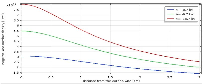
Figure 4-2 shows the space charge density distribution along the radial direction at three different voltages: -8.7 kV, -9.7kV and -10.7kV for both investigated models. For all voltage levels, most of the space charge density concentrates near the corona electrode. The concentration decreases until it reaches a very low value near the collecting
electrode. The space charge concentrated near the corona electrode is larger in the model based on Kaptzov’s hypothesis. The difference in the space charge density calculated from the model applying Kaptzov’s hypothesis and the direct ionization criterion increases as the voltage level increases.
b) Space charge density for the model applying direct ionization criterion
Figure 4-2: Space charge density distribution at three different voltage levels for the single species models
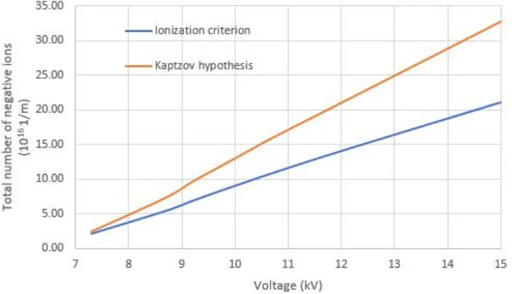
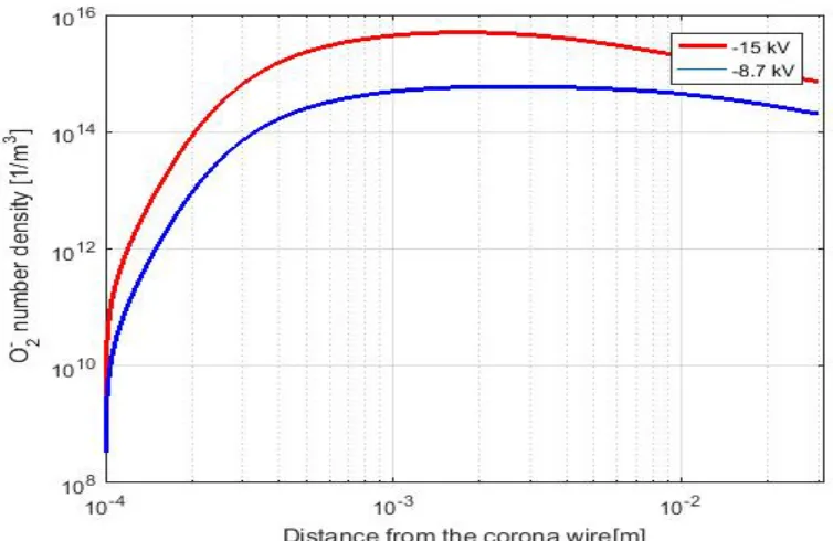
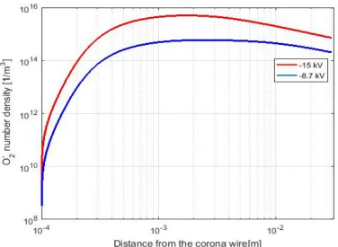
Figure 4-3 shows the total number of the ionic species for different voltages calculated from the models based on the direct ionization criterion and Kaptzov’s hypothesis. The total number of the ionic species for the model using direct ionization approach is smaller than the number obtained from the model using Kaptzov’s hypothesis. As the corona wire voltage increases, the difference between the total number of negative ions resulting from the two models increases until it reaches 53% at -15 kV. Since the electric field resulting from Kaptzov’s hypothesis is lower than that resulting from direct-ionization criterion, more negative-ions are accumulated in the airgap in this model. Charges accumulated closer to the ground electrode have smaller effect on the surface electric field, so a very large difference in the overall number of ions has relatively small effect on the electric field.
4.3
Three-Species Model
The single species corona discharge simulation has been extended to a three-species model, which includes electrons, negative ions and positive ions. A stationary model has been investigated. The voltage-current curve, the electron and ionic species number densities and the electric field distribution for different voltages are presented.
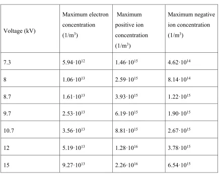
Table 4-1 shows the maximum concentration for the three-ionic species present in this model for different voltage levels. As the voltage increases, the densities of different ions increase.
Table 4-1: Maximum number densities of different species for different voltage levels
Voltage (kV)
Maximum electron concentration (1/m3)
Maximum positive ion concentration (1/m3)
Maximum negative ion concentration (1/m3)
7.3 5.94·1012 1.46·1015 4.62·1014
8 1.06·1013 2.59·1015 8.14·1014
8.7 1.61·1013 3.93·1015 1.22·1015
9.7 2.53·1013 6.19·1015 1.90·1015
10.7 3.56·1013 8.81·1015 2.67·1015
12 5.19·1013 1.28·1016 3.78·1015
15 9.27·1013 2.26·1016 6.54·1015
concentrated near the corona electrode. It is also obvious that the number density of all ions increases as the voltage increases. The exponential increase in the concentration of the electrons near the discharge electrode is caused by the avalanche ionization. This is represented by a linear curve in the log scaled plots. The maximum electron
concentration is reached at approximately the edge of the ionization layer. Starting from that point, the electron concentration starts to decrease, as electrons are attached to neutral molecules.
Positive ions should not exist outside of the ionization layer. However, the numerical model predicts a smooth continuous distribution, so some concentration is predicted there. However, this concentration is a few orders of magnitude smaller and negligible from the practical point of view.
The concentration of negative ions is equal to zero on the discharge electrode. Near the discharge electrode it increases because of the attachment of electrons to neutral
molecules. Starting from some point in the domain, this concentration starts to decrease as no new ions are generated and the total number of ions is distributed over an
a) Electron distribution
c) Negative ions distribution
Figure 4-4: Ionic species distribution for voltage levels of -8.7 kV and -15 kV
4.4
Seven-Species Model
a) Distribution of O-
c) Distribution of O3
e) Distribution of 02+
g) Distribution of 𝑂8^
Figure 4-5: Ionic species distribution of seven-species model for voltages -8.7 kV and -15 kV
Distribution of electrons, and positive and negative O2 ions for this model is not much
different than for the three-species model. One new charge species, O-, shows a
distribution similar to O2-. There are also three neutral species (O, O3 , 01(∇g)) and their
motion is affected by diffusion only. In this situation a uniform distribution would be expected. A slightly non-uniform distribution in one case is caused by numerical errors.
4.5
Electric Field at the Corona Wire
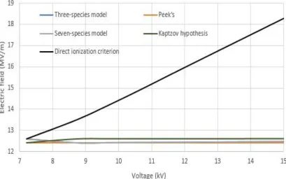
At the onset level, the electric field is high enough for the corona discharge to take place near the corona electrode and all discussed models should predict a very similar value. Figure 4-6 shows the electric field on the corona electrode surface for different voltage levels calculated from different numerical methods. In the case of Kaptzov’s hypothesis, the electric field at the corona electrode should be theoretically the same for any wire voltage. Practically, the values diverge from Peek’s value by about 1.6% due to numerical errors. In the case of the model applying the direct ionization criterion, the electric field at the onset voltage is higher by 2% than Peek’s value. As the voltage increases, the electric field at the corona wire increases until it diverges from Peek’s value by 43.56% for the voltage of -15 kV. For the multi-species models, the difference between the electric field intensity predicted from the seven- and the three-species models are negligible so the two graph lines overlap. At lower voltages, the electric field calculated from multi-species model is about 2% higher than Peek’s value; it satisfies Peek’s formula for voltages higher than -8.3 kV.
4.6
V-I Characteristic Curves
Sato proposed a method to calculate the corona discharge current [61]. This formula is derived from the motion of charged particle between electrodes, and it depends on the energy balance equation.
I = 1
Vo 2πr µb ρ E@@⃗ . E@@@@⃗ dr†
( 4-1)
where 𝜇ˆ is the ion mobility (m2/V·s), ρ is the space charge (C/m3) ,V is the applied
voltage on the corona wire, 𝐸@@@@⃗‰ is the Laplacian electric field (V/m), 𝐸@⃗ is the actual electric field (V/m) , I is the current (A/m) and the integration is done over the radial line connecting both electrodes.
The current in the stationary single-species case can be also calculated by integrating the current density (A/m2), equal to ρµ
bE, on the electrode surface. However, in the 1D case,
no integration is needed. As a result, the total current is is equal to:
I = 2π R i µb ρ E ( 4-2)
The currents resulting from applying equations (4-1) and (4-2) are the same.
To calculate the discharge current for the three-species model, some modifications need to be done to Sato’s equation to account for the added electrons and positive ions species.
𝐼 =1
𝑉o 2𝜋𝑟(𝜇*𝑛*+ 𝜇-𝑛-+ 𝜇ˆ𝑛ˆ ) 𝐸@⃗ . 𝐸@@@@⃗ 𝑑𝑟‰
( 4-3)
The formula for calculating the discharge current should be further expanded to include the ionic species O- in the case of the seven-species model. As a result, Sato’s formula is
as follows:
𝐼 = 1
𝑉o 2𝜋𝑟(𝜇*𝑛*+ 𝜇-𝑛-+ 𝜇ˆ𝑛ˆ + 𝜇••𝑛••) 𝐸@⃗ . 𝐸@@@@⃗ 𝑑𝑟‰
( 4-4)
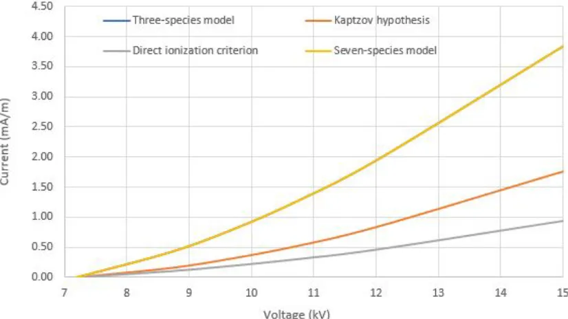
specifically, the corona current is proportional to V· (V-Vonset). Figure 4-7 shows the
currents resulting from the four investigated models. The difference in the current resulting from Kaptzov’s hypothesis and the current obtained from a model using the direct ionization criterion is negligible. Until the voltage -8.3 kV, both currents are the same. Above this voltage, the current resulting from applying Kaptzov hypothesis increases at a higher rate than the current resulting from applying the direct ionization criterion and the difference reaches 1.25 mA/m at the voltage level -15 kV.
The currents resulting from the three-species and seven-species models are very close and the difference is below 0.1%. As a result, both curves overlap on the graph.
On the other hand, the values of the discharge current for different voltage levels obtained from the multipolar models are much higher than the values obtained from the monopolar models. The difference between the currents resulting from the multipolar and monopolar models increases as the applied voltage increases until it reaches a maximum difference of 2 mA/m.
4.7
Conclusions
The negative corona discharge in a wire-cylinder configuration in air has been
numerically investigated in this Chapter. The equations of interest were the drift-diffusion equations for the ionic species and the Poisson equation for the electric field. The
investigated models included single ionic species, three ionic species and seven ionic species. Monopolar model neglected the ionization layer. Kaptzov hypothesis based on Peek’s value and the direct ionization criterion were investigated in this case. The three-species model included the electrons, negative ions 𝑂8^and positive ions 𝑂
8S. In this case,
an iterative algorithm was used and it was necessary to apply an under-relaxation technique in order to have a stable algorithm. The seven-species model included four more ionic species: atomic oxygen O, negative ion of atomic oxygen O-, ozone O
3 and
the excited species O2(1∇g). The voltage-current characteristic curve was plotted for each
investigated model. In addition, Kaptzov’s hypothesis was validated in each case. The spatial distributions of the different ionic species were shown for different voltage levels. The corona current resulting from the three-species model closely agreed with that resulting from the seven-species model. On the other side, a significant difference of the current was reported between the monopolar and multipolar models.
Chapter 5
5
Electrohydrodynamic Flow
The electrohydrodynamic flow produced by the electric corona discharge in atmospheric air has been numerically investigated in a needle to plane configuration. Commercial software, COMSOL, has been used to find the solution of the Poisson’s equation, the three-ionic drift- diffusion equations and Navier-Stokes equation. These equations predict the distributions of electric potential, space charge density and airflow after calculating the volume force. The volume force is the electric Coulomb force, which is the main factor leading to the EHD flow.
5.1 Model Description
5.1.1
Geometry
The investigated model consists of two electrodes. The first electrode is a grounded large metal plate and the second electrode is a sharp needle, perpendicular to the ground electrode and supplied with a high DC negative potential. The needle has a shape of a cylinder ended with a hemisphere. The needle tip radius is 500 µm, the needle body is 5 cm long and the distance between the ground electrode and the tip of the needle is 2 cm. A two-dimensional axisymmetric model is assumed.
5.1.2
Discretization
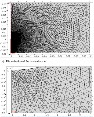
A non-uniform distribution of the electric field in the area close to the corona wire is a critical problem for modeling the corona discharge phenomenon. COMSOL, the software used for simulating the problem, is based on the Finite Element Method. A very fine discretization needs to be used in the area of high field gradient in order to achieve an accurate solution. The mesh should also have a non-uniform distribution; very fine triangular elements are formed near the electrode tip and the size of the elements
a) Discretization of the whole domain
b) Discretization of the domain near the corona tip
Figure 5-1: Discretization of the computational domain
5.1.3
Corona and Flow Model
The simulation algorithm for the corona discharge was discussed in Chapters 3 and 4. Three ionic species have been considered in this model: electrons, positive ions and negative ions. The calculation of the space charge density and the electric field is
essential before simulating the EHD flow, because the Coulomb force is generated by the action of the electric field on the space charge. For the flow model, a laminar flow has been assumed.
5.2
Simulation Results
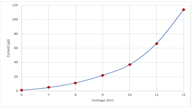
For the investigated model Peek’s value is 7.9 MV/m, which corresponds the onset voltage of -6 kV. Because a stationary case was investigated, the voltage-current characteristics was calculated for the voltages ranging from -6kV to -12 kV. Moreover, the electron and ionic species concentrations, electric field distributions, maximum and minimum velocities for different voltages have been determined.
The voltage-current characteristics is shown in Figure 5-2. The corona current is initiated when the voltage is above the onset voltage, and it changes as a square function of the applied voltage.
Kaptzov’s hypothesis has also been validated in this case. Figure 5-3 shows the value of the electric field on the electrode tip. The electric field is very close to Peek’s value at the onset voltage. However, when the supplied voltage increases, the difference between the actual electric field and Peek’s value increases.
Figure 5-3: Validation of Peek's formula in point-plane configuration
Moreover, comparing the distribution of the electric field along the needle surface with the Peek’s value can give some information about the extent of the ionization area. Figure 5-4 shows the electric field in the area near the needle surface at two voltage levels -8 kV and -12 kV. A close in look to the plots implies that the thickness of the ionization area is about 0.2 mm.
3 5 7 9 11 13 15 17
5.8 6.8 7.8 8.8 9.8 10.8 11.8 12.8
El
ect
ric
fie
ld
(M
V/m
)
Voltage (kV)
a) Electric field near the needle surface at -8 kV
b) Electric field near the needle surface at -12 kV
Figure 5-4: Electric field distribution near the needle surface
a) electron distribution for -8 kV
b) electron distribution for -12 kV
d) positive ions distribution for -12 kV
f) negative ions distribution for -12 kV
Figure 5-5: Distribution of all ionic species in the air gap for voltages -8 kV and -12kV
a) Total number of electrons
b) Total number of positive ions
c) Total number of negative ions
Figure 5-6: Variation of number of different ionic species with voltage
0 1 2 3 4 5 6 7 8 9
6 7 8 9 10 11 12
Tot al num be r of e le ct rons ( 1 0 8) Voltage (kV) 0 2 4 6 8 10 12
6 7 8 9 10 11 12
Tot al num be r of posi tiv e ions ( 1 0 7) Voltage (kV) 0 1 2 3 4 5
6 7 8 9 10 11 12
5.3
Simulation Results of EHD Flow
Figure 5-7 shows the distribution of the magnitude of the EHD force near the needle tip for the voltage levels of -8 kV and -12 kV. The force has a maximum value at the needle tip. It starts decreasing going away from the tip in both r-direction and z-direction. Regarding the direction of the EHD force, the concentration of positive ions is higher than that of the negative ions inside the ionization region. As such, the total charge is positive which implies that the force is directed towards the needle electrode. In the drift zone the net charge is negative, so the Coulomb force is directed towards the ground electrode.
b) Spatial distribution of body force at -12 kV
Figure 5-7: Spatial distribution of body force near the needle tip