A Complex Mix-Shifted Parallel QR Algorithm for the C-Method
Cihui Pan1, 2, 3, Richard Duss´eaux1, *, and Nahid Emad2, 3
Abstract—The C-method is an exact method for analyzing gratings and rough surfaces. This method leads to large-size dense complex non-Hermitian eigenvalue. In this paper, we introduce a parallel QR algorithm that is specifically designed for the C-method. We define the “early shift” for the matrix according to the observed properties. We propose a combination of the “early shift”, Wilkinson’s shift and exceptional shift together to accelerate convergence. First, we use the “early shift” in order to have quick deflation of some eigenvalues. The multi-window bulge chain chasing and parallel aggressive early deflation are used. This approach ensures that most computations are performed in level 3 BLAS operations. The aggressive early deflation approach can detect deflation much quicker and accelerate convergence. Mixed MPI-Open MP techniques are used for performing the codes to hybrid shared and distributed memory platforms. We validate our approach by comparison with experimental data for scattering patterns of two-dimensional rough surfaces.
1. INTRODUCTION
The C-method is an efficient and versatile theoretical tool for analyzing gratings or rough surfaces illuminated by an electromagnetic wave [1–6]. It is based on Maxwell’s equations solved in a non-orthogonal coordinate system fitted to the surface geometry. Discretizing the Maxwell’s equations under a non-orthogonal coordinate system and separating variables lead to solving the eigenvalue problem of the high-dimensional, dense, complex and non-symmetric matrix. The scattered field is expanded as a linear combination of eigensolutions satisfying the outgoing wave condition. The boundary conditions allow the scattering amplitudes to be determined. The strength of the C-method is that it leads to the eigensolutions of the scattering problem. It is an accurate method and it can be used as a reference for the analytical methods [7]. The dominant computational cost for the C-method is the eigenvalue problem solution that is of the order of O(N3) where N is the size of matrix. The C-method must be improved with regard to this point, in particular, for analyzing random rough surfaces insofar as the average scattered intensity is estimated over results of several surface realizations.
In this paper, we focus on the numerical aspects of the C-method in order to reduce the computational time. Iterative eigensolvers, such as Bi-Conjugate Gradient methods, Krylov subspace methods or Jacobi-Davidson methods have been developed to deal with large-scale eigenvalue problems [8]. However, they have the possibility of missing some eigenvalues. Therefore, these iterative methods are inefficient for the C-method because all the eigenvalues and eigenvectors are needed. In contrast, the QR algorithm is based on similarity transformations and calculates all the eigenvalues and eigenvectors without any danger of missing some eigensolutions [9, 10]. We present the parallel QR algorithm that is specifically designed for the C-method. We define a technique, called “early shift” for the matrix according to the properties that we have observed. We mix the “early shift”, Wilkinson’s
Received 8 April 2016, Accepted 11 June 2016, Scheduled 30 June 2016
* Corresponding author: Richard Dusseaux ([email protected]).
shift and exceptional shift together to accelerate the convergence. Especially, we use the “early shift” first to have quick deflation of some eigenvalues [11, 12]. The multi-window bulge chain chasing and parallel aggressive early deflation (AED) are used [12, 13]. A Mixed Message Passing Interface and Open Multi-Processing techniques (Mixed MPI-Open MP) are utilized for parallel implementation of our application for hybrid shared and distributed memory platforms [14, 15].
The paper is structured as follows. In Section 2, we present the C-method. In Section 3, we introduce the parallel QR algorithm specifically designed for the C-method and we present the implementation details, architectures and platforms. In Section 4, we present numerical experiments and we validate numerical results by comparison with experimental data.
2. THE C-METHOD AS AN EIGENVALUE PROBLEM
2.1. Formulation of the Problem
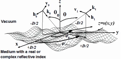
Consider a periodic surface with a height profilez=s(x, y) and a periodDwith respect toOx andOy axis (See Figure 1). The surface separates the vacuum (ν(1)= 1) from a material with a reflective index
ν(2). It is illuminated by a monochromatic plane wave with wavelength λ(1). The time-dependence
factor varies as exp(jωt) where ω is the angular frequency. Each vector function is represented by its associated complex vector function and the time factor is omitted. Superscripts (1) and (2) designate quantities relative to the upper medium and the lower medium, respectively. The incident wave vector
k0 is defined from the zenith angle θ0 and the azimuth angle ϕ0 [4]. For an incident wave in (a)
polarization, the problem consists in working out the co- and cross-polarized components of the field scattered within the two media.
Figure 1. An elementary cell of a periodic surface illuminated by a plane wave under (θ0, ϕ0). h0 and v0 are the polarization vectors of the incident plane wave. In the vacuum, the diffracted elementary wave is characterized by the wave vectork1, the polarization vectorsh1 and v1, the zenith angleθand the azimuth angle ϕ[3, 4].
The C-method uses the translation coordinate system (u, v, ω) where (u, v) = (x, y) and w =
z−s(x, y). So, the height function z = s(x, y) coincides with the coordinate surface w = 0 and the change from Cartesian components (ax; ay; az) of a vectora to covariant components (au, av, aw) is given by [1, 3]. ⎧
⎪ ⎪ ⎪ ⎨ ⎪ ⎪ ⎪ ⎩
au(x, y, w) =ax(x , y , z) + ∂s(x, y)
∂x az(x , y , z) av(x , y, w) =ay(x;, y , z) +∂s(x, y)
∂y az(x , y , z) aw(x , y, w) =az(x , y , z)
(1)
equations and the constitutive relations expressed in the translation system that the componentψ=Ew orψ=ZHw obeys to the propagation equation:
∂2ψ ∂u2 +
∂2ψ ∂v2 +gww
∂2ψ ∂w2 +k
2ψ+ ∂ ∂w
guw∂ ψ
∂u +
∂ guwψ
∂u +gvw ∂ ψ
∂v +
∂ gvwψ
∂v
= 0 (2)
k is the wave number of the medium under consideration andZ, this impedance. Termsguw,gvw and
gww are elements of metric tensor which depend on the derivatives of function s(u, v) with respect tou and v [3].
guw =−∂s
∂u gvw=−∂s
∂v
gww= 1 +∂s
∂u 2 + ∂s ∂v 2 (3)
As shown in [3],Eu,Ev,Hu and Hv can be expressed in terms ofEw and Hw only:
∂2E
u
∂w2 +k 2E
u = ∂
2E
w
∂u∂w −k2guwEw−jk
gvw∂ZHw ∂w +
∂ZHw
∂v (4)
∂2E
v
∂w2 +k 2E
v = ∂
2E
w
∂v∂w −k2gvwEw+jk
guw∂ZHw ∂w +
∂ZHw
∂v (5)
∂2H
u
∂w2 +k 2H
u = ∂
2H
w
∂u∂w −k2guwHw+j k Z
gvw∂Ew ∂w +
∂Ew
∂v (6)
∂2H
v
∂w2 +k 2H
v = ∂
2H
w
∂v∂w −k2gvwHw−j k Z
guw∂Ew
∂w + ∂Ew
∂v (7)
2.2. Eigenvalue System
In [3], a procedure is proposed for solving the propagation Equation (2). ψ(x, y, w) is represented in terms of the quasi-periodic functions exp(−jαpx) exp(−jβqy):
ψ(x, y, w) = p
q
ψpq(w)exp(−jαpx) exp(−jβqy) (8)
where
αp =k(1)sinθ0cosϕ0+p
2π
D, βq=k(1)sinθ0sinϕ0+q
2π
D (9)
Substituting (8) and (9) into (2) and projecting on the quasi-periodic functions gives:
j k(1) ∂ ∂w p,q α s
k(1)g
uw
s−p,t−q+gsuw−p,t−qkα(1)p + βt k(1)g
vw
s−p,t−q+gvws−p,t−qkβ(1)q ψpq(w) + j k(1) ∂ ∂w p,q gww
s−p,t−qψpq(w)
= γ
2
st
k(1)2ψst(w) (10)
where
j k(1)
∂ψpq(w)
∂w =ψpq (w) (11)
and γst2 =k2−α2s−βt2. It is interesting to note thatγstis the propagation coefficient of an elementary plane wave with respect to the Oz axis [1]. Termsgp,quw,gp,qvw and gwwp,q are the Fourier coefficients of the periodic functionsguw,gvw and gww. Equations (10) and (11) can be written in matrix form:
j k(1)Ll
∂ ∂w
ψ
ψ =Lr
ψ
ψpq and ψpq are the components of vectors ψ and ψ. For a truncation order M, −M ≤ p, q ≤ +M. As a result, Ll and Lr are 2Ms-square matrices with Ms = (2M+ 1)2. The elementary solution of Equation (12) is defined as follows:
ψn(w)
ψ
n(w) =
φ
n
φ
n
exp(−jk(1)rnw) (13)
φnand φn are the upper eigenvector and the lower eigenvector associated with the eigenvaluern. They are solutions of the eigenvalue problem (14).
rnLl
φ
n
φ
n
=Lr
φ
n
φ
n
(14)
System (14) gives 2Ms eigensolutionsψn(x, y, w) defined as follows:
ψn(x, y, w) =
+M
p=−M +M
q=−M
ϕn,pqexp(−jαpx) exp (−jβqy) exp
−jk(1)r
nw
(15)
For each medium (m), the C-method requires the solution of an eigenvalue problem. The signs of the real and imaginary parts of the eigenvalue define the nature of the wave corresponding to the elementary wave function (15). ψn(m)(x, y, w) represents an outgoing wave travelling without attenuation if Re
(−1)mr(nm))
<0 and Im(r(nm)) = 0. For an evanescent wave, Im
(−1)mr(nm))
>0.
The componentψs(m)(x, y, w) of the field scattered within the medium (m) is expanded as a linear combination of eigensolutions ψ(nm)(x, y, w) satisfying the outgoing wave condition. Among the 2Ms eigenfunctions, there are Ms of them that correspond to outgoing waves and as many of them to incoming waves.
ψ(m)
s (x, y, w) = Ms
n=1 A(m)
n ψn(m)(x, y, w) (16)
For an incident wave in (a) polarization, we deduce from Eq. (4) to Eq. (7) the (ha)-polarized components (Esu(m,ha), Esv(m,ha), Hsu(m,ha), Hsv(m,ha)) by taking Esw(m) = 0 and Hsw(m) = ψ(sm). The (va )-polarized components (Esu(m,va), Esv(m,va), Hsu(m,va), Hsv(m,va)) by takingEsw(m) =ψs(m)andHsw(m)= 0. The co-amplitudesA(naa) and the cross-amplitudesA(nba)are found by solving the boundary value problem and a 2Ms-dimensional matrix system. In this section, we have succinctly presented numerical implementation of the C-method. For more information, we refer the reader to Reference [3] for 2D-gratings and to References [4–6] for 2D random rough surfaces.
3. ALGORITHMS
The most time-consuming part of C-method is to compute the eigenvalues and eigenvectors ofA=L−r1Ll where A is a large size, complex, dense and non-Hermitian matrix. For determining the complete spectrum, the most powerful and stable algorithm is the QR algorithm [8–10]. We choose this algorithm to keep the stability and to save the computation time.
the bulge). In general, as the complement to the use of the shift, the deflation technique is used in the QR algorithm. This means that once an eigenvalue has converged, the corresponding rows and columns of the Hessenberg matrix will be removed and thus, the following QR iterations will be applied on a smaller matrix.
We make use of three techniques in the implementation of our parallel QR algorithm: early shift, parallel bulge chasing and parallel aggressive early deflation (AED). We introduce in parallel QR algorithm, the early shifts to give approximation of a part of the eigenvalues of the matrix. For the bulge chasing, instead of only a single bulge, containing two shifts, a chain of several tightly coupled bulges, each containing two shifts, is chased in the course of one multi-shift QR iteration [11, 12]. This idea allows performing most of the computational work in terms of matrix-matrix multiplications to benefit from highly efficient level 3 basic linear algebra subprograms (BLAS, the level 3 contains matrix-matrix operations) [16]. The idea of AED allows to detect converged eigenvalues much earlier than conventional deflation strategies. We will first present QR sequential algorithm and the shift strategy to accelerate the convergence, then we present all the parallel techniques for this specifically designed QR algorithm.
3.1. Double Shifted QR Algorithm
The QR algorithm is an iterative method for reducing a matrix to almost upper triangular form by unitary similarity transformations. The idea is to compute the Schur decomposition of a N-square complex matrix A (here, N = 2Ms with Ms = (2M + 1)2): T = WHAW [9] where T is an upper triangular matrix andWH is the conjugate transpose of W which is the Schur matrix of A. Formally, let A0 := A. A0 := A. At the k-th step (starting with k = 0), we compute the QR decomposition: Ak = QkRk where Qk is an unitary matrix and Rk is an upper triangular matrix. We then form
Ak+1 =RkQk and:
Ak+1 =RkQk=QHkAkQk (17)
So all the matrices Ak are similar to each other and hence they have the same eigenvalues. By this iteration, the matrices Ak converge to an upper triangular matrix, the Schur form of A. Usually, the QR algorithm starts with the Hessenberg decomposition [10]:
H=QHAQ (18)
H is a Hessenberg matrix and Qis a unitary matrix. This is because the Hessenberg form is preserved by the QR algorithm and this form can decrease the cost of the QR iterations [10]. There are several ways of Hessenberg reduction such as Gram-Schmidt transformation, Householder reduction and Givens rotation [10]. Efficient parallel algorithm for this Hessenberg reduction is implemented in the ScaLAPACK (Scalable Linear Algebra PACKage) routine PZGEHRD [17]. So we will focus on the iterative part that comes after this Hessenberg reduction.
The convergence of the Hessenberg QR algorithm can be improved dramatically by introducing spectral shifts into the algorithm. Nevertheless, in some cases, the shifted Hessenberg QR algorithm does not work well. For the single shift, when the element hN−1,N−1 of the Hessenberg matrix H is
negligible with respect to hN,N−1, the convergence could be slow even if the Rayleigh quotient shift
gives a very good approximation (e.g., hN,N−1 is very small). For this reason, we make use of double
shifted Hessenberg QR algorithm. This technique is also used for real matrices with complex conjugate eigenvalues because it allows avoiding the introduction of complex numbers in calculations during QR iterations. Indeed, the so-called implicit Q theorem allows us to use the implicit double shift QR algorithm without explicitly computing the QR decomposition [10]. The algorithm is characterized by a “bulge chasing” procedure.
Suppose that two shiftsσ1 andσ2 of the Hessenberg matrixH are given. The implicit double shift
a) Calculate the first column of the shift polynomial
v= (H−σ1I)(H−σ2I)e1 = ⎛ ⎜ ⎜ ⎜ ⎜ ⎜ ⎝ ∗ ∗ ∗ 0 0 ⎞ ⎟ ⎟ ⎟ ⎟ ⎟ ⎠ (19)
b) Construct a 3×3 Householder transformation Q1 such that the second and third entries of v are
transformed to zero (i.e.,Q1v). The similarity transformation gives the updated matrix H1:
H1=QH1 HQ1 = ⎛ ⎜ ⎜ ⎜ ⎜ ⎜ ⎜ ⎜ ⎝ ∗ ∗ ∗ ∗ ∗ ∗ ↔
X X X ∗ ∗ ∗ ↔
X X X ∗ ∗ ∗ ↔
X X X ∗ ∗ ∗ ↔
0 0 0 ∗ ∗ ∗ ↔
0 0 0 0 ∗ ∗ ↔
⎞ ⎟ ⎟ ⎟ ⎟ ⎟ ⎟ ⎟ ⎠ (20)
The Hessenberg structure is damaged by the bulge that we denote with symbol “X”.
c) Construct a 3×3 Householder transformationQ2 such that the third and fourth entries of the first
column of H1 reduce to zero. The similarity transformation gives the updated matrixH2:
H2=QH2 H1Q2 = ⎛ ⎜ ⎜ ⎜ ⎜ ⎜ ⎜ ⎜ ⎝ ∗ ∗ ∗ ∗ ∗ ∗ ↔ ∗ ∗ ∗ ∗ ∗ ∗ ↔
0 X X X ∗ ∗ ↔
0 X X X ∗ ∗ ↔
0 X X X ∗ ∗ ↔
0 0 0 0 ∗ ∗ ↔
⎞ ⎟ ⎟ ⎟ ⎟ ⎟ ⎟ ⎟ ⎠ (21)
d) Continue similar operations to chase the bulge. In general, construct a 3 × 3 Householder transformationQk such that the (k+ 1)th and (k+ 2)th entries of the (k−1)th column of Hkare mapped to zero. Applying the corresponding similarity transformation to Hk results the updated matrix Hk+1 where k = 2,3, . . . , N −1. The bulge will be chased to vanish at the bottom right
corner and leads to zeros, thus deflations. For example,H3 will be look like as follows:
H3 =QH3 H2Q3 = ⎛ ⎜ ⎜ ⎜ ⎜ ⎜ ⎜ ⎜ ⎝ ∗ ∗ ∗ ∗ ∗ ∗ ↔ ∗ ∗ ∗ ∗ ∗ ∗ ↔
0 ∗ ∗ ∗ ∗ ∗ ↔
0 0 X X X ∗ ↔
0 0 X X X ∗ ↔
0 0 X X X ∗ ↔
⎞ ⎟ ⎟ ⎟ ⎟ ⎟ ⎟ ⎟ ⎠ (22)
3.2. Early Shift
Some eigenvalues of the scattering matrix can be approximated as follows [1]:
r(m)
n ≈ ±γ˜pq(m)=±
ν(m)2−α˜2
p−β˜q2 (23)
where ˜αp = αp/k(1), ˜βq = βq/k(1) and ˜γpq(m) = γpq(m)/k(1). As shown in [1], the values ˜γpq(m) constitute very good approximations when the indexes p and q are small relative to the matrix size. In general, ifn(m) is real or has a very small imaginary part, for the pair (p, q) that satisfies ˜α2p+ ˜βq2 <Re(ν(m)), the approximation can be quite accurate. We recall that for a lossless medium (m), a real value ˜
γ(m)
˜
βq = sinθ(nm)sinϕ(nm) and ˜γpq(m) = ±cosθ(nm) (see Figure 1). The real eigenvalue r(nm) defines the propagation direction of the eigenfunction ψ(nm)(x, y, w). In [1], this approximation is used in order to describe the asymptotic scattered field in the lossless medium by a sum of elementary plane waves propagating without any attenuation. As shown in [1], this procedure is numerically efficient.
Here, the expression of ˜γpq(m) can be used as shifts to approximate the real eigenvalues or eigenvalues with very small imaginary part. The convergence is very quick due to the good approximation. We call this the “early shift”. This specific shift is used in pairs corresponding to above double shift QR algorithm. One pair of the “early shift” will create a bulge to be chased. Each pair will be used only once during one iteration of double shifted Hessenberg QR which corresponds to (n−1) right and left multiplications ofA by Householder reflectors. Wilkinson shift can be used after the “early shift” [10]. The “early shift” represents a further step forward in relation to previous works on the C method.
3.3. Parallel QR with Tightly Coupled Bulge Chasing
The parallel bulge chasing algorithm was first proposed by Braman et al. [11]. In order to benefit from the level 3 BLAS, they parallelize the bulge chasing procedure by performing the chasing of multiple chains of tightly coupled bulges. With the delay and accumulate technique, the main computation work becomes the matrix-matrix multiplications. The procedure of intra-block chasing and inter-block chasing are described below.
To describe the parallel algorithm, we first introduce the data layout mapping in a distributed memory environment as follows:
• The processors are arranged into apr×pc rectangular mesh labeled from (0,0) to (pr−1, pc−1) according to their specific positions indices in the mesh. Usually the values ofpr and pc are set to be as close as possible.
• TheN×N matrix is partitioned in 2D block cyclic scheme [17] and is mapped on ourpr×pc grid. The block size isMb×Nb and we require the block to be square Mb =Nb. Generally, a processor will store a collection of non-contiguous blocks. Figure 2 shows an example with a fourth-order grid wherepr =pc = 2. The four processors are represented by different colors. If the matrix size isN = 16, then the block size is 4x4 and the processor (0, 0) will store the elements A(1 : 4,1 : 4),
A(1 : 4,9 : 12), A(9 : 12,1 : 4) and A(9 : 12,9 : 12). An array descriptor stores the details of data layout. The mapping between entries of the global matrix and their corresponding locations in the memory can be established from the array descriptor.
Figure 2. 2D block cyclic scheme with four processors andpr =pc = 2.
Locally, each processor in the mesh may also utilize multithreading often associated with shared memory architectures. This can be seen as adding another level of explicit parallelization by organizing all the pr×pc processors into a three-dimensional mesh [12].
We use the shifts that are mentioned earlier to introduce the chain of bulges into diagonal blocks. Each of the chains resides on a different diagonal block. We choose the number of shifts in such a way that each chain covers at most half of the data layout block. The “early shift” is distributed from left-upper diagonal blocks to right-lower diagonal blocks. Each “early shift” is used once. When there is no “early shift” to distribute, we use Wilkinson shift [10].
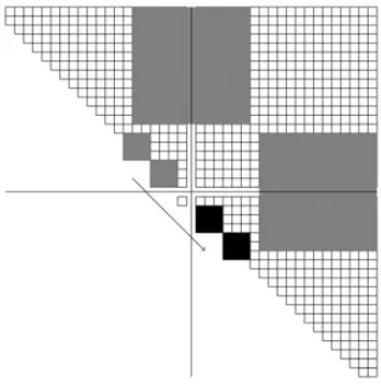
Figure 3. Intra-block parallel bulge chasing. The grey bulges are chased to the black bulges. The matrix under consideration is a 40×40 matrix. It is partitioned into 4 square blocks of size 20×20.
to chase the chain of bulges down some rows to the down right-hand corner of the contiguous diagonal block. We start from the lowest bulge of the block and chase one bulge at a time. The intra-block chasing can be performed locally on the process that owns this chain and simultaneously between different diagonal contiguous blocks that saves computation time. Figure 3 shows how the intra-block chasing are performed, the grey bulges are chased to the black bulges. After the bulge chasing within the diagonal block, the accumulated unitary matrices are sent to the corresponding processors in order to update the off-diagonal blocks. The off-diagonal blocks are then updated by matrix-matrix multiplications that use level 3 BLAS. The broadcasts are sent in parallel. In order to avoid conflicts in the intersecting parts, they are performed first in the row direction and then in the column direction (See Figure 3 for the intra-block chasing with pr =pc = 2 and Mb=Nb= 20).
For the inter-block chasing, for each diagonal blocks in which the bulge chains reside, we create copies of its neighbors and it becomes similar to the case of intra-block chasing. Figure 4 illustrates the procedure with pr = pc = 2 and Mb = Nb = 20, the grey bulges are chased to the black bulges. More precisely, the processor that stores the grey bulges creates a copy of the block on each side of the border. Then we can perform the chasing locally, just as in the intra-block chasing and broadcast the corresponding orthogonal factors to the blocks on both sides of the cross border. The updated neighboring blocks are sent to its owner. To update the corresponding off-diagonal blocks, we broadcast orthogonal matrix accumulated in the diagonal chasing stage to the corresponding rows/columns of processors that are involved in off-diagonal updating. Then each involved processor exchanges data blocks with its neighbor as illustrated in Figure 4 in the two large gray blocks. The off-diagonal blocks are then updated by multiplication with the accumulated orthogonal matrix. We perform inter-block chasing first for the odd-numbered blocks and then for the even-numbered blocks. This odd-even manner avoids conflicts between different tightly coupled chains [12].
For each diagonal block, the corresponding orthogonal transformations are accumulated into an orthogonal factor. Each orthogonal has the following form:
U =
U11 U12
U21 U22 (24)
U12is a lower triangular matrix andU21is a upper triangular matrix. As a result, matrix multiplications
Figure 4. Inter-block parallel bulge chasing. The dark grey large parts exchange data blocks with neighbors when updating off-diagonal blocks.
3.4. Parallel AED
The AED algorithm was proposed in [13]. We divide the Hessenberg matrixH as follows:
H=
H
11 H12 H13 H21 H22 H23
0 H32 H33
(25)
where H11 and H33 are (N −k−1)-and k-square matrices, respectively. We use the pipeline parallel
QR algorithm to find the Schur decomposition of H33 with H33 = V T VH and perform the following
similarity transformation:
⎛
⎝ I0 01 00 0 0 VH
⎞ ⎠
H
11 H12 H13 H21 H22 H23
0 H32 H33
I 0 0 0 1 0 0 0 V
=
H
11 H12 H13V H21 H22 H23V
0 s T
(26)
I is the (N−k−1)-square identity matrix andT an upper triangular k-square matrix. Now the matrix looks like as in Figure 5 where the spike sis denoted as the gray part.
3.5. Hardware and Software Platforms
For the sequential case, there are two stages: the Hessenberg matrix implementation and the triangular decomposition of the Hessenberg matrix. Each of these stages requires one matrix and a few buffers with “negligible” sizes for intermediate calculations. For the parallel QR case, the matrix is distributed over the computation nodes. It is necessary to store it somewhere and to update it regularly. We must therefore store at most two matrices and we need a few buffers for the intermediate calculations. The computer memory required is proportional to N2.
The experiments are performed on the machine Poincare hosted by IDRIS national computing center in France (http://www.idris.fr/). This machine is IBM computer, composed mainly iDataPlex dx360 M4 servers: 92 nodes equipped with 2 Sandy Bridge E5-2670 processors (2.60 GHz, 8 cores every processor, 16 cores every node) and 32 Gb memory every node.
Figure 5. Aggressive early deflation. The grey spike contains the vectors.
4. NUMERICAL RESULTS
4.1. Surfaces under Consideration
The parallel QR algorithm presented in Section 3 can be used for analyzing crossed gratings or two-dimensional random gratings. As an illustration, we consider in this section periodic random surfaces having a Gaussian height distribution. The correlation function is Gaussian and isotropic. We noteσs the root mean square height of the surface andls, the correlation length, respectively. For an incident wave in (a) polarization and a scattered wave in (b) polarization, the average scattered intensity in the upper medium is derived from the scattering amplitudesA(nba)associated with angles (θn,ϕn) [18]. The average scattered intensity is estimated by averaging the scattering amplitudes over Nr realizations. The interface realization is obtained by filtering of uncorrelated white noise [18, 19].
4.2. Reduction on the Computational Time
To compare the computation times of sequential algorithm and parallel algorithm, we present Figure 6 that is based on numerical result of one realization. The perfectly conducting surface we consider is of 64 square wavelengths and σs = λ(1) and ls = √2λ(1). The incident angle is chosen as θ0 = 30◦ and ϕ0= 0◦. The truncation orderM is equal to 28 and the matrix size is N= 6498.
Figure 6 gives the results of the pairs (pr;pc) = (1; 1) (2; 2) (4; 4) (6; 6) and (8; 8). Considering one core, the proposed algorithm with respect to the sequential one leads to a substantial reduction in the computational time (factor higher than 5). With the new version of parallel strategy by using 16 cores for one simulation, the solutions for 100 eigenvalues problems associated with 100 surface realizations require approximately 12 minutes if we use 1600 cores. The naive parallel strategy based on using the sequential algorithm and on solving of individual realizations on individual processors requires approximately 330 minutes. The proposed parallel strategy can be significantly more efficient than the naive parallel strategy.
2.6 2.8 3 3.2 3.4 3.6 3.8 4 4.2 4.4
0 10 20 30 40 50 60 70
Computation time (log10(seconds))
#Cores
Parallel: Sequential:
Figure 6. Computation times with respect to number of cores.
0 5000 10000 15000 20000 25000
10 15 20 25 30 35 40
Computation time (seconds)
M
Parallel: Sequential:
Figure 7. Computation times with respect to truncation order.
4.3. Comparison with Experimental Data
We use the parallel QR algorithm for analyzing random grating and we compare numerical results with published experimental data considering random rough surfaces. We analyze moderately rough and very rough surfaces. For all simulations, D= 8λ, M = 28 and Nr = 200. First, we consider a surface with a moderate roughness,σs= 0.352λ(1) and ls = 2.21λ(1), and illuminated under θ0 = 55◦ and ϕ0 = 0◦.
The reflective index of the lower medium is ν(2) = 1.62−0.001j. Figure 8 shows the (vv)-polarized differential reflection coefficient (DRC) as a function of the observation angle in the incidence plane [20]. It is noteworthy that the DRC curve presents a minimum similar to the Brewster angle for a planar surface (By analogy with reflection from a smooth surface, a lossless dielectric with a refractive index equal to 1.62 provides a Brewster angle close to 58◦). The comparison with experimental data that come from [20] is excellent. The comparison is also conclusive for (hh)-results.
0 0.002 0.004 0.006 0.008 0.01 0.012 0.014 0.016 0.018 0.02
-20 0 20 40 60 80 100
DRC
Scattering Angle (deg) C-method:
Exp:
Figure 8. Differential reflection coefficient versus observation angle in the incidence plane. Moderately rough surface. Polarization (vv).
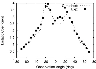
Figure 9 shows the (vv)-polarized normalized bistatic cross section as a function of the observation angle in the incidence plane for a perfectly conducting surface [21]. Figure 10 gives results for the (hv)-polarized bistatic cross section. We consider a very rough surface for which the predictions of the standard analytic methods are inaccurate [7]. Roughness parameters are: σs = λ(1) and l
s = √2λ(1) and the surface is illuminated underθ0 = 20◦ and ϕ0 = 0◦. The C-method used with M = 28 leads to
an error on the power balance smaller than 5% for all the realizations. The mean error estimated over the 200 realizations is smaller than 2×10⁻³.
0 0.5 1 1.5 2 2.5 3 3.5 4
-80 -60 -40 -20 0 20 40 60 80
Bistatic Coefficient
Observation Angle (deg) C-method:
Exp:
Figure 9. Normalized bistatic scattering cross section versus observation angle in the incidence plane. Very rough surface. Polarization (vv).
0 0.2 0.4 0.6 0.8 1 1.2 1.4 1.6 1.8 2
-80 -60 -40 -20 0 20 40 60 80
Bistatic Coefficient
Observation Angle (deg) C-method:
Exp:
Figure 10. Normalized bistatic scattering cross section versus observation angle in the incidence plane. Very rough surface. Polarization (hv).
for the first surface realization, the relative errors are small and vary within the range [10−8, 10−3]. With early shift, the computational time of parallel multi-shift and AED decreases by approximately 16%.
It is noteworthy that the studied surface exhibits backscattering enhancement in both co-polarized and cross-polarized returns. We recall that the truncation order is a numerical parameter of the C-method. The Mth-order truncation removes the evanescent waves in the field components as shown in Equations (15) and (16). The evanescent waves contribute to the near field and take part in the couplings between propagating waves. For the roughness parameters under consideration, when we use the C-method with M = 28, the proportion of the evanescent wave functions is sufficient to describe the electromagnetic couplings and to analyze the backscattering enhancement. The comparison with experimental data coming from [21] is very good and the backscattering peaks coincide well. The comparison is also conclusive for (hh)- and (vh)-results.
5. CONCLUSION
In this paper, we have proposed a parallel QR algorithm that is specifically designed for the C-method applied to the scattering of electromagnetic plane wave by a rough surface. From numerical experiments, we have observed that some eigenvalues can be approximated efficiently by the propagation coefficients of elementary plane waves with respect to the Oz axis. We design the “early shift” algorithm to take advantage of this property. We plug this “early shift” method, together with Wilkinson shift and exceptional shift, into the new parallel QR algorithm. This algorithm uses multiple chains of tightly coupled bulges chasing technique to parallelize the conventional bulge chasing and the aggressive early deflation technique to detect deflation quickly. We apply this specifically designed parallel QR algorithm to the matrix characterizing the scattering problem. We also compare the computation time with that of the sequential code. The proposed algorithm leads to a substantial reduction in the computational time.
This parallel QR algorithm can be used for analyzing crossed gratings or two-dimensional random gratings. In this paper, we have analyzed two-dimensional random rough surfaces by a grating approach. Comparisons with experimental data are conclusive in both co- and cross-polarized components and validate the grating approach for moderately rough and very rough surfaces under consideration.
REFERENCES
1. Chandezon, J., D. Maystre, and G. Raoult, “A new theoretical method for diffraction gratings and its numerical application,” J. Optics (Paris), Vol. 11, 235–241, 1980.
3. Granet, G., “Analysis of diffraction by surface-relief crossed gratings with use of the Chandezon method: Application to multilayer crossed gratings,”J. Opt. Soc. Am. A, Vol. 15, 1121–1131, 1998. 4. A¨ıt Braham, K., R. Duss´eaux, and G. Granet, “Scattering of electromagnetic waves from two-dimensional perfectly conducting random rough surfaces — Study with the curvilinear coordinate method,”Waves Random Complex Media, Vol. 18, 255–274, 2008.
5. Duss´eaux, R., K. A¨ıt Braham, and G. Granet, “Implementation and validation of the curvilinear coordinate method for the scattering of electromagnetic waves from two-dimensional dielectric random rough surfaces,” Waves Random Complex Media, Vol. 18, 551–570, 2008.
6. Duss´eaux, R., E. Vannier, O. Taconet, and G. Granet, “Study of backscatter signature for seedbed surface evolution under rainfall — Influence of radar precision,” Progress In Electromagnetics Research, Vol. 125, 415–437, 2012.
7. Elfouhaily, T. M. and C. A. Gu´erin, “A critical survey of approximate scattering wave theories from random rough surfaces,”Waves in Random and Complex Media, Vol. 14, R1–10, 2004. 8. Bai, Z., J. W. Demmel, J. J. Dongarra, A. Ruhe, and H. van Der Vorst,Templates for the Solution
of Algebraic Eigenvalue Problems. Software, Environments, and Tools, SIAM, 2000.
9. Golub, G. H. and F. Uhlig, “The QR algorithm: 50 years later its genesis by John Francis and Vera Kublanovskayaand subsequent developments,”IMA J. Numer. Anal., Vol. 29, 467–485, 2009. 10. Golub, G. H. and C. F. Van Loan, Matrix Computations, Johns Hopkins University Press,
Baltimore, 1996.
11. Braman, K., R. Byers, and R. Mathias, “The multi-shift QR algorithm. Part I: Maintaining well-focused shifts and level 3 performance,” SIAM J. Matrix Anal. Appl., Vol. 23, 929–947, 2002. 12. Granat, R., B. Kagstr¨om, and D. Kressner, “A novel parallel QR algorithm for hybrid distributed
memory HPC systems,”SIAM J. Sci. Comput., Vol. 32, 2345–2378, 2010.
13. Braman, K., R. Byers, and R. Mathias, “The multi-shift QR algorithm. Part II: Aggressive early deflation,” SIAM J. Matrix Anal. Appl., Vol. 23, 948–972, 2002.
14. “MPI — Messaging passing interface,” See http://www.mcs.anl.gov/research/projects/mpi/. 15. “OpenMP — Open multi-processing,” See http://openmp.org/wp/.
16. “BLAS — Basic linear algebra subprograms,” See http://www.netlib.org/blas/.
17. “ScaLAPACK — Scalable linear algebra package,” See http://www.netlib.org/scalapack/.
18. Kong, J. A., K. H. Ding, and C. O. Ao, Scattering of Electromagnetic Waves — Numerical Simulations, Wiley-Interscience, New York, 2001.
19. Afifi, S. and R. Duss´eaux, “Scattering by anisotropic rough layered 2D interfaces,” IEEE Trans. Antennas Propag., Vol. 60, 5315–5328, 2012.
20. Berginc, G., “Small-slope approximation method: A further study of vector wave scattering from two-dimensional surfaces and comparison with experimental data,” Progress In Electromagnetics Research, Vol. 37, 251–287, 2002.