An Efficient Method for Solving Frequency Responses
of Power-Line Networks
Bing Li*, Daniel M˚ansson, and Guang Yang
Abstract—This paper presents a novel approach for solving the frequency responses of a power-line network, which is a two-parallel-conductor system with multiple junctions and branches. By correcting the reflection coefficient and transmission coefficient of each junction, a complex network can be decomposed into several, single-junction, units. Based on the Baum-Liu-Tesche (BLT) equation, we preliminarily propose the calculation method of frequency responses for single-junction network. In accordance with the direction of power transfer, we calculate the frequency responses of loads connected to each junction sequentially, from the perspective of the network structure. This approach greatly simplifies the computational complexity of the network frequency responses. To verify the proposed algorithm, networks with various numbers of junctions and branches are investigated, and the results are compared with a commercial electromagnetic simulator based on the topology. The analytical results agree well with the simulated ones.
1. INTRODUCTION
For the frequency response calculation of a power-line network, Anatory et al. [1–5] gave the transfer function of power-line networks from excitation source to load responses, establishing an overall model of broadband power-line communication network with irregularly distributed branched networks, arbitrary terminal loads, various line lengths and characteristic impedances. This method gives the relationships of voltages and currents between transmitting and receiving ends, but it cannot be applied to simultaneously obtain the frequency responses at other terminal loads. Also, to take the effects of all the other loads into account, the calculation equations require to be nested for relatively more times than the method proposed in this paper.
Due to the multiple junctions in the power-line network, there are multiple reflections between junctions, which results in a multi-path propagation in the network, and the theoretical number of the propagation paths is infinite. After listing the probable propagation paths between the transmitter and receiver as much as possible, Ding and Meng [6] derived the transfer function by using a recursive model. However, it is merely suitable for the point-to-point case and the accuracy of the model depends on the selection of the number of multiple reflections. Considering the effects of the adjacent junctions, Shin et al. [7] defined a degree of distantness, where the junctions are not in the direct propagation path linking the transmitting and receiving terminals. However, the complexity of the network increases with the number of the adjacent junctions or the branches connected to the adjacent junctions, and the accuracy of the model is heavily affected by the choice of the degree of distantness. Departing from the perspective of two-port networks, Zheng et al. [8] established the power-line channel model that solves the matrix equations of the network and obtains the frequency responses of target load, by using the admittance matrix as well as the relationship between branch admittance matrix and node admittance matrix.
Received 30 January 2015, Accepted 23 April 2015, Scheduled 4 May 2015 * Corresponding author: Bing Li ([email protected]).
Originating in the EMC community, the Baum-Liu-Tesche (BLT) equation [9–14], proposed by Baum, Liu and Tesche, can also be applied to solve this kind of problem. The equation describes the electromagnetic waves leaving and entering junctions, and the wave propagation along tubes in a transmission-line network, by using the scattering matrix and propagation matrix of the network. But the scattering parameter between two waves is difficult to obtain, as any wave is the superposition of many other waves. In addition, conventional methods do not work when facing the super matrix equations in Zheng’s model [8] and the BLT model [9–14] above. Besides, a super matrix requires fairly large space for storage and its computation is time-consuming.
In our study, a more efficient approach based on the BLT equation is proposed to solve the frequency responses. The calculation results include all load frequency responses at each termination. The main idea is to divide a complex power-line network with arbitrary structure into multiple local single-junction units, instead of establishing a global model which includes the relationships between all loads. In the single-junction model, there are no multiple reflections, hence there is no need to provide any approximation on the number of reflections. By adopting a tree structure in the algorithm, all junctions and loads at the layer is simultaneously computed, in the processes of coefficients correction and frequency responses calculation, and the algorithm converges fast even if the network is fairly complex.
2. METHODS OF CALCULATING LOAD RESPONSES
In a power-line network, with the number of arbitrary distributed junctions and branches increasing, the complexity of the network increases. Different branch lengths, load values and line characteristic impedances also increase the diversity of the network configuration. In our study, with respect to various network complexities, six typical power-line networks shown in Figure 1 are investigated, and the calculation of the frequency responses at each load will be discussed subsequently in the following sections.
In this paper, In represents the n×n identity matrix, 0 the matrix with entries 0, diag(∗) the diagonal matrix, and adiag(∗) the anti-diagonal matrix. (∗) and (∗) respectively denote the real part and the imaginary part of a complex number, and (∗)T stands for transpose.
2.1. The BLT Equation
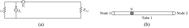
To solve the frequency responses, for the simplest power-line network (see Figure 1(a)), the BLT equation [11] is applied. Assuming that the line length is L, propagation constant is γ, characteristic impedance isZc, and the load impedances areZL1 andZL2, respectively. The excitation source consists
of a lumped voltage source Vs and a lumped current source Is, which are located at a distance of xs
from the left load ZL1 (see Figure 2).
When the excitation source (VsandIs) act on the power-line, the voltage waves propagate along the
power-line. Note that the voltage consists of the incident waves Vinc = [V1inc, V2inc]T and the reflected wavesVref = [V1ref, V2ref]T shown in Figure 3, by following the BLT equation in the matrix way, we have
Vinc =ΓVref+S, (1)
where Γ = adiage−γL, e−γL. Besides,S = [S1, S2]T in (1) represents the excitation vector, which is
given by
S 1
S2
=
⎡ ⎢ ⎣ −
1
2(Vs−ZcIs)e
−γxs
1
2(Vs+ZcIs)e
−γ(L−xs) ⎤ ⎥ ⎦.
Generally, the propagation constant γ =jωμ(σ+jω) is a complex number. Let α=(γ) and
β =(γ) be the attenuation constant and phase constant, respectively. According to [15], we have
α=ω
μ
2
1 +
σ
ω
2
−1
1/2
and β=ω
μ
2
1 +
σ
ω
2
+ 1
1/2
#1 #2 Excitation
(a)
#1
#2
#3 #4
Excitation
(b)
#1
#2 #3
#4 Excitation
(c)
#1
#2 #3
#4
#5
#6 #7 #8
#9 #10
#11 Excitation
#1
#2 #3
#4
#5
#6 #7 #8 #9 #10
#11 #12
#13
#14
#15
Excitation
#15
#14 #9
#10
#3
#4 #5 #1 #2 #6
#7 #8
#11
#12
#13
Excitation
(f)
(d) (e)
Figure 1. Different types of power-line network. (a) Two loads without junction; (b) four loads with one junction; (c) four loads with two junctions; (d) eleven loads with five junctions; (e) fifteen loads with seven junctions; and (f) fifteen loads with seven junctions with different excitation.
Vs
ZL1 Is ZL2
Node 1 Node 2
Vs
Tube 1
(a) (b)
Figure 2. The network of Figure 1(a). (a) Geometry; and (b) tube model.
Here, ω is angular frequency, and μ, and σ are permeability, permittivity and conductivity of the medium between two conductors in a transmission line. Particularly, if the media is lossless, that is
σ= 0, then α and β are reduced to
α= 0 and β =ω√μ= ω
v =
2πf
v =
2π
λ , (2)
#1 #2
1 ref
V
1 inc
V
2 inc
V
2 ref
V
Figure 3. Voltage travelling waves on the power-line.
Following the transmission line theory, the incident voltage and reflected voltage at a load satisfies
Vref =ρVinc, (3)
whereρ is the reflection coefficient shown as
ρ= ZL−Zc
ZL+Zc
. (4)
Thus, in the network shown in Figure 1(a), given the reflection coefficients ρ1 and ρ2 at two terminals
respectively, the reflected voltage can be expressed as
Vref =PVinc, (5)
whereP= diag (ρ1, ρ2).
Note that the frequency responses V= [V1, V2]T is the superposition of the incident and reflected
voltages, say
V=Vinc+Vref, (6)
by combining (1), (5) and (6), we finally obtain the frequency responses by
V= (I2+P) (I2−ΓP)−1S. (7)
2.2. The Modified BLT Equation
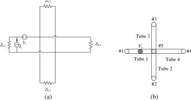
In this section, we extend our case to the network with one junction and four branches, as shown in Figure 4. At the branch i, i = 1,2,3,4, the length is Li, the propagation constant is γi, and the characteristic impedances are Zci. Besides, at the end of the branchi, the load is given byZLi, which
has the same index with branch. The excitation sources are located on the first branch.
Due to the junction in this network, the BLT equation needs to be modified. We suppose that TEM is the main mode of wave propagation, and if this mode is dominant also through the junction (as seen in [16]), then the reflection can be described by the transmission line theory. The voltage travelling waves propagate along all branches connected to a junction, since they are connected in parallel. The
Vs
ZL1
ZL3
ZL2
ZL4
Is
'
(a)
#1
#3
#2
#4 #5
Vs
Tube 1 Tube 3
Tube 2 Tube 4
(b)
...
reflection coefficients ρ(i) and the transmission coefficients T(i) for each branch at the junction, where the superscript icorresponds to the branchi, are respectively given by
⎧ ⎪ ⎪ ⎪ ⎪ ⎪ ⎪ ⎪ ⎪ ⎪ ⎪ ⎪ ⎨ ⎪ ⎪ ⎪ ⎪ ⎪ ⎪ ⎪ ⎪ ⎪ ⎪ ⎪ ⎩
ρ(1)= Zc2//Zc3//Zc4−Zc1
Zc2//Zc3//Zc4+Zc1
ρ(2)= Zc1//Zc3//Zc4−Zc2
Zc1//Zc3//Zc4+Zc2
ρ(3)= Zc1//Zc2//Zc4−Zc3
Zc1//Zc2//Zc4+Zc3
ρ(4)= Zc1//Zc2//Zc3−Zc4
Zc1//Zc2//Zc3+Zc4
and ⎧ ⎪ ⎪ ⎪ ⎪ ⎨ ⎪ ⎪ ⎪ ⎪ ⎩
T(1) = 1 +ρ(1)
T(2) = 1 +ρ(2)
T(3) = 1 +ρ(3)
T(4) = 1 +ρ(4)
, (8)
Note that, for n parallel-connected power line with characteristic impedance Zk, k = 1,2, . . . , n, we have
Z1//Z2//. . .//Zn= n
k=1
Z−1
k
−1
, (9)
without loss of generality, for anyi∈ {1,2,3,4}, the reflection coefficients and transmission coefficients in (8) can be formulated as
ρ(i)= ⎛ ⎝
j=i
Z−1 cj
⎞ ⎠
−1
−Zci ⎛
⎝
j=i
Z−1 cj
⎞ ⎠
−1
+Zci
and T(i) = 1 +ρ(i). (10)
Particularly, if the branches have the identical characteristic impedance, say Zci = Zc, i= 1,2,3,4,
the reflection coefficient ρ(i) at each branch can be reduced to
ρ(i) = Zc/3−Zc
Zc/3 +Zc =− 1
2. (11)
Based on the reflection coefficient and the transmission coefficient at the junction, we modify the original BLT equation. Similar to the analysis in Section 2.1, for the voltage travelling waves shown in Figure 5, we have the relationship between the incident voltages and the reflected as shown in (1), with Vinc = [V1inc, V2inc, V3inc, V4inc]T,Vref= [V1ref, V2ref, V3ref, V4ref]T, the transmission matrix
Γ= ⎡ ⎢ ⎢ ⎢ ⎣
ρ(1)e−2γ1L1 T(2)e−(γ1L1+γ2L2) T(3)e−(γ1L1+γ3L3) T(4)e−(γ1L1+γ4L4)
T(1)e−(γ1L1+γ2L2) ρ(2)e−2γ2L2 T(3)e−(γ2L2+γ3L3) T(4)e−(γ2L2+γ4L4)
T(1)e−(γ1L1+γ3L3) T(2)e−(γ2L2+γ3L3) ρ(3)e−2γ3L3 T(4)e−(γ3L3+γ4L4)
T(1)e−(γ1L1+γ4L4) T(2)e−(γ2L2+γ4L4) T(3)e−(γ3L3+γ4L4) ρ(4)e−2γ4L4
⎤ ⎥ ⎥ ⎥
⎦, (12)
#1 #2 #3 #4 ref 1 V inc 1 V ref 2
V V2inc inc
3
V V3ref
inc 4 V ref 4 V
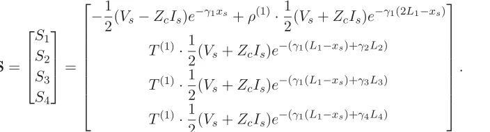
and the excitation vector
S=
⎡ ⎢ ⎢ ⎣
S1
S2
S3
S4 ⎤ ⎥ ⎥ ⎦=
⎡ ⎢ ⎢ ⎢ ⎢ ⎢ ⎢ ⎢ ⎢ ⎣
−1
2(Vs−ZcIs)e
−γ1xs+ρ(1)·1
2(Vs+ZcIs)e
−γ1(2L1−xs)
T(1)·1
2(Vs+ZcIs)e
−(γ1(L1−xs)+γ2L2)
T(1)·1
2(Vs+ZcIs)e
−(γ1(L1−xs)+γ3L3)
T(1)·1
2(Vs+ZcIs)e
−(γ1(L1−xs)+γ4L4)
⎤ ⎥ ⎥ ⎥ ⎥ ⎥ ⎥ ⎥ ⎥ ⎦
. (13)
Additionally, given the reflection coefficient ρi at the terminali,i= 1, 2,3,4, we have
P= diag (ρ1, ρ2, ρ3, ρ4). (14)
Following the relationships for the reflected and incident waves in (1) and (5), as well as the superposition law in (6), we similarly obtain the frequency response matrixV= [V1, V2, V3, V4]T as
V= (I4+P) (I4−ΓP)−1S. (15)
Comparing (15) with (7), we can easily find that they have the same form of expression, but with completely different matrices (vectors).
3. UNIT CALCULATION METHOD BASED ON COEFFICIENT CORRECTION
Here, a power-line network with multiple junctions is discussed. We take the network with two junctions and four branches (loads) as an example and conduct the analysis, and subsequently develop an algorithm for computing multiple distributed junctions and branches. Within the network shown in Figure 1(c), we assume the branch lengths, propagation constants, characteristic impedances and load values are distinct. The excitation source is still located on the first branch. Besides, the length of the line between the two junctions isL.
The algorithm idea consists of two steps. We first divide the network into two single-junction network units, as shown in Figure 6. The cut is located at the second junction, and the equivalent
#1
#2 #3
#4 Excitation
#2 ' #4
#1
#2
#3' Excitation
(a)
(b) (c)
#3
loads in two units are labelled as 3 and 2, respectively. To hold the structure of the second unit, i.e., ensure that there are still three branches connected to the junction, a virtual branch of length zero is introduced to the second junction. For the single-junction network shown in Figure 6(b), we use the modified BLT equation to solve the load responses. Afterwards, according to the transfer direction of power, the power absorbed by the load 3 is put as the excitation source of the second single-junction network, and compute the load responses in the second unit. More details are provided in the following parts.
3.1. Coefficient Correction
To calculate the frequency responses of the first unit, the reflection coefficient and the transmission coefficient are required. At the second junction of the network shown in Figure 6(a), the coefficients can be obtained by using (8). To take the circled part shown in Figure 7 as a super load, the effects of load 3 and load 4 need to be taken into account.
For the super load, we setS=0 since no excitation source participates. Considering the length of the virtual branch is zero, by applying (12), we obtain
⎡ ⎢ ⎣ Vref 3 Vinc 3 Vinc 4 ⎤ ⎥ ⎦= ⎡ ⎢ ⎢ ⎣
T2−1 T2(3)e−γ3L3 T
(4) 2 e−γ4L4
T2e−γ3L3 ρ(3)2 e−2γ3L3 T (4)
2 e−(γ3L3+γ4L4)
T2e−γ4L4 T (3)
2 e−(γ3L3+γ4L4) ρ (4)
2 e−2γ4L4 ⎤ ⎥ ⎥ ⎦ ⎡ ⎢ ⎣ Vinc 3 Vref 3 Vref 4 ⎤ ⎥
⎦, (16)
whereρ(3)2 ,ρ(4)2 are the reflection coefficients, andT2,T (3) 2 ,T
(4)
2 are the transmission coefficients at the
second junction for the connected line and two branches. The superscript represents the branch index and the subscript is junction number.
Besides, by following the definition of reflection coefficient, we have
Vref 3 Vref 4 =
ρ3 0
0 ρ4
Vinc 3 Vinc 4 , (17)
whereρ3 andρ4 are the reflection coefficients at load 3 and 4, respectively. Substituting (17) into (16),
the corrected reflection coefficient for the load 3 is derived as
ρ3 V ref 3
Vinc 3
= (T2−1) + T2T (3) 2 A 1− T(3) 2 A + T(4) 2 B
+ T2T
(4) 2 B 1− T(3) 2 A + T(4) 2 B , (18)
whereA= 1+ 1
ρ3e−2γ3L3
,B = 1+ 1
ρ4e−2γ4L4
. From (18), we can see that the calculation of the reflection coefficient for the super load 3 involves the terminal load reflection coefficients, propagation constants, branch lengths and branch transmission coefficients.
#1 #2 #3 #4 1 ref V 1 inc V 2 ref V 2 inc V 3ref
V 3 inc V inc V ref V 4 inc V 4 ref V 3' 3'
Figure 7. Voltage travelling waves in the network of Figure 1(c).
#1 #2 inc V ref V #N #3
Without loss of generality, for the junction withN+ 1 branches, as shown in Figure 8, the corrected coefficient at the junction is
ρ = (T −1) +
T
T(1)
A1
+T
(2)
A2
+. . .+T
(N)
AN
1−
T(1)
A1
+T
(2)
A2
+. . .+T
(N)
AN
=T
1− N
i=1
T(i)
Ai
−1
−1 =T−1, (19)
whereAi= 1+ 1
ρie−2γiLi,T
(i)is the transmission coefficients for branchi, andTdenotes the transmission
coefficient for the connected line. Here, T is regarded as the equivalent transmission coefficient, from the angle of the connected line to characterize the single-junction unit.
3.2. Calculation of Frequency Response at Each Load
The calculation of the frequency response at each load runs recursively. In our specific model, since we decompose the network into two units, we should first solve the unit one, regarding the load 1, 2 and 3. After obtaining the frequency response at load 3, we access the unit two to compute the frequency responses of the loads in unit two.
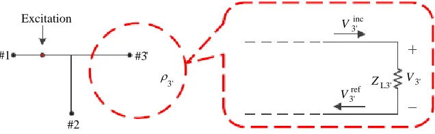
(1) For Unit One: there are three branches connected to the junction. Supposing that the value of the super load 3 isZL3, the equivalent model is shown in Figure 9. By applying the modified BLT
approach proposed in Section 2.2, we obtain the frequency responses at the three loads.
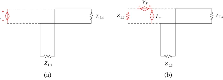
(2) For Unit Two: we use the frequency responses of load 3 as excitation source, as shown in Figure 10(a). SinceV3 is a voltage determined by Unit One, the symbol of the controlled voltage source
is used here. The length of the virtual branch where the excitation source are placed is set to zero. To apply the modified BLT equation, we construct a network similar to the one shown in Figure 4(a). Therefore, the location of the excitation source shifts to the placexs away from the terminal. Because
the length of the virtual branch is zero, the value of xs should also be zero. In addition, to show the
integrity of analysis, technically we add an equivalent controlled current source (see Figure 10(b)) at the same position of the controlled voltage source, but the value of the current should be zero. Considering that the terminal of the virtual branch is shorted, a virtual load, ZL2, is added at the terminal, as
shown in Figure 10(b), and the load value is zero. According to (4), the reflection coefficient is set to be ρ2 = −1. Then, the frequency responses of the loads in unit two are obtained. So far, all load
frequency responses in the entire network are solved.
#1
#2
#3' Excitation
ref 3'
V
inc 3'
V
3'
V
3' ZL3'
ρ
Figure 9. Equivalent model of the super load.
4. ALGORITHM
L3 Z 3'
V
L3 Z
Z L2'
Z
3' V
3' I L4
Z
(a) (b)
L4
Figure 10. The second unit of the network. (a) The second unit with equivalent excitation source; and (b) deformation of the second unit.
4.1. Algorithm Description
In what follows, we develop an algorithm that is applied to the complex power-line networks with multiple distributed junctions and branches, such as the networks in Figure 1(e) and Figure 1(f), aiming at computing the frequency response in an efficient way.
Taking the network in Figure 1(e) as an example, there are three main branches, seven junctions and fifteen branches with loads. It is evident that the network is tree-structured and can be displayed in the topology given by Figure 11. The junction that connects to the excitation source is placed at the top point, and is set to be root node of the tree. Throughout the tree, there are totally seven layers, which is one more than the height of the tree.
Given that we have the knowledge of all load values, branch lengths, junctions and the excitation
J1
J2 #2 #1
J3 #4 #3
J4 #7 #6
J6 J5 #9
#5
#8
J7 #12 #11 #10
#15 #14 #13
source, the algorithm consists of two phases and the main steps are outlined as follows:
(i) From the bottom to the top: recursively correct the reflection coefficient at junctions on the upper layer until the root (top point) is reached;
(ii) From the top to the bottom: after correcting all the reflection coefficients, recursively calculate the load response for the associated child nodes until the bottom layer is reached.
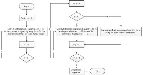
For a tree-structured network with n layers, the procedure of the algorithm is illustrated in Figure 12.
4.2. Algorithm Complexity Analysis
Given a tree-structure network of heightn, equivalently n+ 1 layers, we denote by Xi,i= 1,2, . . . , n, the set of child nodes number for the parents at layer i. To be more precise, at layer i, assuming there areli parents, thenXi is shown as
Xi ={Xi,1, Xi,2, . . . , Xi,li}, (20)
whereXi,k,k= 1,2, . . . , li, corresponds to the number of child nodes for thekth parent at layer i. To quantify the algorithm efficiency, a straightforward and effective way is to count the number of arithmetic operations (i.e., the addition and multiplication) when conducting the calculation. Based on the complexity metric given above, we analyze the efficiency performance of the following three methods: our proposed method, the recursive time domain method [6], and simulations made with the numerical software, EMEC [17]. As we will discuss, those three schemes are all involving the matrix inversion, which contributes most among all possible operations in terms of the computational complexity.
Although the time complexity of matrix inversion can be improved through designing related algorithms (as stated in [18, 19], the steps of arithmetic operations of inversion or multiplication for a matrix of order m are bounded by O(mw), where 2 < w ≤ 3 is determined by the algorithms. Here, the notation O(∗) describes the limiting behaviour of a function when the argument tends towards a particular value or infinity, which is widely used in time complexity analysis to classify algorithms [20, 21]), we here take the Gaussian-Jordan elimination method for matrix inversion as
Begin
i < 2
Correct all the reflection coefficients of the father nodes at layer i, by using the reflection
coefficients at their associated child nodes
i = i − 1
N
Compute the load responses at layer (j + 1), by setting the reflections coefficients of the
ancestor node at layer (j − 1) as −1
j= j + 1
Y Compute the load responses at layer (j + 1), by
using the input source information
j > 1 N
j > n − 1
End Output load
responses Set i = n − 1
Set j = 1
N
Y
Y
the standard approach to obtain the matrix inversion, whose number of arithmetic operations can be expressed [22] as f(N) = 3k=1akNk, where ak, k = 1,2,3, are certain scalars such that f(N) is monotonically increasing withN, andN is the order of matrix. Commonly, we consider the worst case to test the complexity of algorithm, then the numbers of additions and multiplications are respectively given by [23]
fA(N) = 13N3+12N2−56N and fM(N) = 13N3+N2+13N, (21)
thus the total operations is
f(N)fA(N) +fM(N) = 2 3N
3+3
2N
2−1
2N ≈ ˜
f(N) 2 3N
3, for N 1. (22)
where ˜f(N) is an approximation of f(N) for sufficiently large N. For the sake of simplicity, in the following analysis, we adopt the metric ˜f(∗) to evaluate the complexity.
• In our proposed algorithm, we assume each parent node has the capability of processing data locally, individually, then the total number of operationsM1 is given by:
M1= 2
n i=1 li j=1
f(Xi,j)≈2 n i=1 li j=1 ˜
f(Xi,j) = 4 3 n i=1 li j=1 X3 i,j (23)
where the factor 2 comes from the round-trip procedure, i.e., from bottom to top, then back to bottom.
• By the recursive time domain solution proposed in [6], we need to establish a globalN×N matrix Ato represent the reflection/transmission coefficients, and the orderN is twice of edges in the tree graph, say
N = 2m= 2 n i=1 li j=1
X(i)
j . (24)
Note that the recursive time domain solution involves the multipath, strictly speaking, to achieve the perfect ideal theoretical results of load responses, we should consider all potential paths. In graph theory and matrix theory, we follow the concept of transition matrix to verify if the destination is reachable after several transitions. To be more precise, in [6], the reflection/transmission matrix coefficient matrix A is the transition matrix, and the following operation to calculate the frequency response value is recursively multiplying A and conducting the superposition on the derived values of each iteration. Equivalently, the manipulation can be summarized by lim K→∞ K i=0
Ai =IN +A+A2+· · ·= (IN −A)−1, (25)
where K is referred to as the iterations, IN is an identity matrix of size N. It is easy to see, the above closed-form expression derives the load response with perfect precision. In this manner, the
M2 ≈f˜(N) =
2 3 ⎛ ⎝2 n i=1 li j=1 Xi,j ⎞ ⎠ 3 > 16 3 n i=1 ⎛ ⎝li
j=1 Xi,j ⎞ ⎠ 3 > 16 3 n i=1 li j=1 X3
i,j ≈4M1 (26)
• In the software EMEC, nodal analysis is used. The employed algorithm is based on the admittance matrix for the whole network, which is inverted into a system impedance matrix, and the voltage in all nodes is calculated by multiplying the impedance with the current vector [17]. Note that, the order of the admittance matrix is the number of all nodes (including the root node), thus, following the previous notations, we have the N×N admittance matrix with
N =m+ 1 = n i=1 li j=1
X(i)
it is easy to show that, the metricM3 satisfies
M1 <M3≈f˜(N) =
2 3
⎛ ⎝1 +
n
i=1
li
j=1
Xi,j
⎞ ⎠ 3
<M2 (28)
In light of above analysis, we observe, for the distributed calculation methods (i.e., the first scheme), the complexity merely relies on the maximum degree of the tree graph, however, the subsequent two algorithms require the sum of all degrees. Obviously, given the fixed height of tree-structured network
n, by increasing the number of loads, we can see that,M1 M3 <M2, which implies the significant
improvement in efficiency.
5. COMPARISON OF CALCULATING RESULTS
To validate the algorithm, we take the commercial software EMEC [17] as the benchmark, which is based on electromagnetic topology. For test purpose, the parameters chosen for the variables in the power-line networks are given in Table 1–Table 5. The characteristic impedances for each power line are all 45 Ω, which are consistent with the cable data given in the datasheet of the software EMEC.
Table 1. Parameters for the network shown in Figure 1(a).
Parameter Load (Ω) Length (m) Distance (m) Voltage (V) Current (A)
ZL1 ZL2 L xs Vs Is
Value 200 400 10 1 100 0
Table 2. Parameters for the network shown in Figure 1(b).
Parameter Load (Ω) Length (m) Distance (m) Voltage (V) Current (A)
ZL1 ZL2 ZL3 ZL4 BL1 BL2 BL3 BL4 xs Vs Is
Value 10 10 100 200 10 10 10 10 5 100 0
Table 3. Parameters for the network shown in Figure 1(c).
Parameter Load (Ω) Length (m) Distance (m) Voltage (V) Current (A)
ZL1 ZL2 ZL3 ZL4 BL1 BL2 BL3 BL4 L xs Vs Is
Value 10 10 100 200 10 10 10 10 10 5 100 0
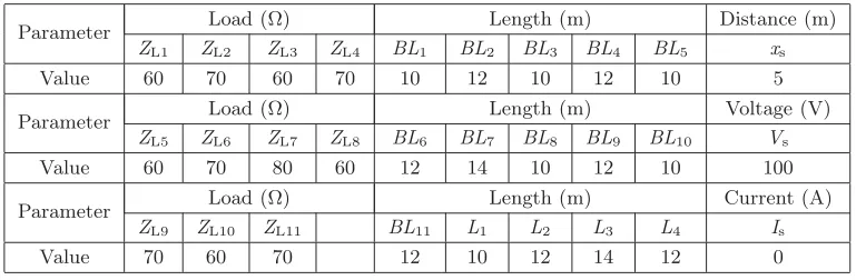
Table 4. Parameters for the network shown in Figure 1(d).
Parameter Load (Ω) Length (m) Distance (m)
ZL1 ZL2 ZL3 ZL4 BL1 BL2 BL3 BL4 BL5 xs
Value 60 70 60 70 10 12 10 12 10 5
Parameter Load (Ω) Length (m) Voltage (V)
ZL5 ZL6 ZL7 ZL8 BL6 BL7 BL8 BL9 BL10 Vs
Value 60 70 80 60 12 14 10 12 10 100
Parameter Load (Ω) Length (m) Current (A)
ZL9 ZL10 ZL11 BL11 L1 L2 L3 L4 Is
Table 5. Parameters for the network shown in Figure 1(e) and Figure 1(f).
Parameter Load (Ω) Length (m) Distance (m)
ZL1 ZL2 ZL3 ZL4 ZL5 BL1 BL2 BL3 BL4 BL5 BL6 BL7 xs
Value 60 70 60 70 60 10 12 10 12 10 12 14 5
Parameter Load (Ω) Length (m) voltage (V)
ZL6 ZL7 ZL8 ZL9 ZL10 BL8 BL9 BL10 BL11 BL12 BL13 BL14 Vs
Value 70 80 60 70 60 10 12 10 12 10 10 12 100
Parameter Load (Ω) Length (m) Current (A)
ZL11 ZL12 ZL13 ZL14 ZL15 BL15 L1 L2 L3 L4 L5 L6 Is
Value 70 60 60 70 80 14 10 12 14 12 10 12 0
0 0.2 0.4 0.6 0.8 1 1.2 1.4 1.6 1.8 2 ×10⁷ Load response
Frequency [Hz] #1(M)
#2(M) #1(E) #2(E)
20 40 60 80 100 120 140 160 180 200
Voltage [V]
Figure 13. Calculation results of the network shown in Figure 1(a).
0 0.2 0.4 0.6 0.8 1 1.2 1.4 1.6 1.8 2 ×10⁷ Load response
Frequency [Hz] #1(M) #2(M) #3(M) #4(M) #1(E) #2(E) #3(E) #4(E)
0 10 20 30 40 50 60 70 80 90
Voltage [V]
Figure 14. Calculation results of the network shown in Figure 1(b).
0 0.2 0.4 0.6 0.8 1 1.2 1.4 1.6 1.8 2 ×10⁷ 0
10 20 30 40 50 60 70 80 90
Load response
Frequency [Hz]
Voltage [V]
#1(M) #2(M) #3(M) #4(M) #1(E) #2(E) #3(E) #4(E)
Figure 15. Calculation results of the network shown in Figure 1(c).
0 0.2 0.4 0.6 0.8 1 1.2 1.4 1.6 1.8 2 ×10⁷ 0
10 20 30 40 50 60 70 80 90 100
Load response
Frequency [Hz]
Voltage [V]
#1(M) #2(M) #3(M) #5(M) #8(M) #10(M)
Figure 16. Calculation results of the network shown in Figure 1(d).
0 0.2 0.4 0.6 0.8 1 1.2 1.4 1.6 1.8 2 ×10⁷ 0
10 20 30 40 50 60 70 80 90 100
Load response
Frequency [Hz]
Voltage [V]
#1(M) #2(M) #3(M) #5(M) #8(M) #13(M)
Figure 17. Calculation results of the network shown in Figure 1(e).
0 0.2 0.4 0.6 0.8 1 1.2 1.4 1.6 1.8 2 ×10⁷ Load response
Frequency [Hz] #1(M) #3(M) #6(M) #8(M) #11(M) #14(M)
0 10 20 30 40 50 60
Voltage [V]
Figure 18. Calculation results of the network shown in Figure 1(f).
results show that, the frequency responses from the algorithm and the EMEC software coincide very well. This agreement shows the proposed method is accurate. The maximum error found in any studied case presented here is less than 5%.
6. CONCLUSION
We study the conventional approaches in computing the frequency responses and point out their application limitations when the power-line network grows complex. Based on the classic BLT equation, we conduct the corresponding modifications to make it applicable to the scenarios with one junction as well as multiple ends. We further propose a generic and efficient algorithm for computing the frequency responses at each load in complex power-line networks with multiple distributed junctions and branches with loads. The key idea of the algorithm is to deal the whole network with an equivalent composition of units. The reflection coefficients can be recursively achieved by regarding the units as the super loads, and the frequency responses at each load can be eventually obtained by recursively entering the units and applying the modified BLT equation locally. Results comparison shows that the algorithm converges fast and highly coincides with solutions by the EMEC software. Compared to the graphical interface based EMEC software, the proposed algorithm is much easier for the implementation as well as the adjustment of power-line network structure with various parameters.
REFERENCES
1. Anatory, J., N. Theethayi, and R. Thottappillil, “Power-line communication channel model for interconnected networks — Part I: Two-conductor system,” IEEE Trans. Power Del., Vol. 24, No. 1, 118–123, 2009.
2. Anatory, J., N. Theethayi, R. Thottappillil, et al., “A broadband power-line communication system design scheme for typical Tanzanian low-voltage network,”IEEE Trans. Power Del., Vol. 24, No. 3, 1218–1224, 2009.
3. Anatory, J., N. Theethayi, R. Thottappillil, et al., “Expressions for current/voltage distribution in broadband power-line communication networks involving branches,” IEEE Trans. Power Del., Vol. 23, No. 1, 188–195, 2008.
4. Anatory, J., N. Theethayi, R. Thottappillil, et al., “An experimental validation for broadband power-line communication (BPLC) model,” IEEE Trans. Power Del., Vol. 23, No. 3, 1380–1383, 2008.
6. Ding, X. and J. Meng, “Channel estimation and simulation of an indoor power-line network via a recursive time-domain solution,”IEEE Trans. Power Del., Vol. 24, No. 1, 144–152, 2009.
7. Shin, J., J. Lee, and J. Jeong, “Channel modeling for indoor broadband power-line communications networks with arbitrary topologies by taking adjacent nodes into account,” IEEE Trans. Power Del., Vol. 26, No. 3, 1432–1439, 2011.
8. Zheng, T., M. Raugi, and M. Tucci, “Time-invariant characteristics of naval power-line channels,”
IEEE Trans. Power Del., Vol. 27, No. 2, 858–865, 2012.
9. Baum, C. E., “How to think about EMP interaction,” Proceedings of the 1974 Spring FULMEN Meeting, 1974.
10. Baum, C. E., T. K. Liu, and F. M. Tesche, “On the analysis of general multiconductor transmission-line networks,” Interaction Note 350, 467–547, 1978.
11. Baum, C. E., “Generalization of the BLT equation,”Proc. 13th Zurich EMC Symp., 131–136, 1999. 12. Tesche, F. M., “Topological concepts for internal EMP interaction,” IEEE Trans. AP, Vol. 26,
No. 1, 1978.
13. Tesche, F. M., “Development and use of the BLT equation in the time domain as applied to a coaxial cable,”IEEE Trans. EMC, Vol. 49, No. 1, 3–11, 2007.
14. Tesche, F. M. and C. M. Butler, “On the addition of EM field propagation and coupling effects in the BLT equation,”Interaction Notes, 2004.
15. Paul, C. R.,Introduction to Electromagnetic Compatibility, A Wiley Interscience Publication, USA, 1992.
16. M˚ansson, D., R. Thottappillil, and M. B¨ackstr¨om, “Propagation of UWB transients in low-voltage power installation networks,” IEEE Trans. EMC, Vol. 50, No. 3, 619–629, 2008.
17. Carlsson, J., T. Karlsson, and G. Und´en, “EMEC — An EM simulator based on topology,” IEEE Trans. EMC, Vol. 46, No. 3, 353–358, 2004.
18. Coppersmith, D. and S. Winograd,, “Matrix multiplication via arithmetic progressions,”
Proceedings of the Nineteenth Annual ACM Symposium on Theory of Computing, 1–6, 1987. 19. Pan, V., “Complexity of parallel matrix computations,” Theoretical Computer Science, Vol. 54,
No. 1, 65–85, 1987.
20. Black, P. E., “Big-O notation,”Dictionary of Algorithms and Data Structures, 2007.
21. Mohr, A., “Quantum computing in complexity theory and theory of computation,” 1–6, 2014, www.austinmohr.com/Work files/complexity.pdf.
22. Valiant, L. G., “The complexity of computing the permanent,” Theoretical Computer Science, Vol. 8, No. 2, 189–201, 1979.