An improved parallel AGE method to solve incomplete blow-up problem through high performance computing system

Int. J. Open Problems Compt. Math., Vol. 3, No. 3, September 2010 ISSN 1998-6262; Copyright © ICSRS Publication, 2010

www.i-csrs.org

An Improved Parallel AGE Method to Solve

Incomplete Blow-up Problem through High

Performance Computing System

Norma Alias1, Md. Rajibul Islam2, Nurul Ain Zhafarina Muhamad3, Noriza Satam3 and Norhafiza Hamzah3

1_{Ibnu Sina Institute, Faculty of Science, University Technology Malaysia, 81310}

Johor

e-mail: [email protected]

2_{Faculty of Information Science and Technology, Multimedia University,}

Malaysia

e-mail: [email protected]

3_{Mathematic Department, Faculty of Science, University Technology Malaysia,}

81310 Johor

e-mail: {nurul.ain.zhafarina, norizasatam, norhafizahamzah}@gmail.com

Abstract

Incomplete blow-up is a condition under the quasilinear heat equation. The Porous Medium Equation (PME) with power source are admitting incomplete blow-up. It is used as one of the filtration process in the industry. This filtration process has been used globally in the medical and laboratory applications. Previously, the standard numerical procedure was Gauss Seidel method to solve this problem. We propose a new variance of the Alternating Group Explicit Scheme (AGE) algorithms to solve incomplete blow-up problem through High performance computing (HPC). HPC systems include of multiple (usually mass-produced) processors linked together in a single system with commercially available interconnects. This is in contrast to mainframe computers, which are generally monolithic in nature. Four important terms that are, convergent rate by the number of iteration, execution time, computational complexity and stability are considered in this study to evaluate the performances of this approach.

1 Introduction

Temperature distribution is a physical model may be imagined in which heat is considered to be a fluid inside matter, free to flow from one position to another. The amount of fluid present is measured in some unit such as the calorie (cal) or BTU (British Thermal Unit). Evidence of its presence in matter is the temperature thereof; it is assumed that the more heat presents the higher the temperature, and that it flows from places of high temperature to places of low temperature. Temperature can be measured directly by a thermometer; the quantity of heat present is inferred indirectly.

Five types of blow-up patterns were illustrated for the 4th-order semilinear parabolic equation of reaction-diffusion type by Galaktionov [1] and Noriko Mizoguchi [2] presented multiple blow-ups to solve a semilinear heat equation problem. R. Natalini, C. Sinestrari and A. Tesei [3] presented an incomplete blowup of entropy solutions to first-order quasilinear hyperbolic balance laws. They specified a general procedure to continue solutions beyond the blowup time, which made use of monotonicity methods. The continuations thus obtained were possibly unbounded and satisfied suitable generalized entropy and Rankine-Hugoniot conditions. Then they proved the uniqueness of continuations satisfying such conditions as well. José M. Arrieta and Aníbal Rodríguez-Bernal [4] showed that blow-up occurred only on the boundary while they analyzed the existence of solutions that blow-up in finite time for a reaction-diffusion equation. Noriko Mizoguchi and Juan Luis Vazquez [5] demonstrated multiple blow-ups for semilinear heat equations at different places and different times and also solutions for a semilinear heat equations II described by Noriko Mizoguchi [6]. Nonlinear Volterra integral equations of the second kind with solutions that blow-up or quench had analyzed by Catherine A. Roberts [7].

1.1 Incomplete

Blow-up

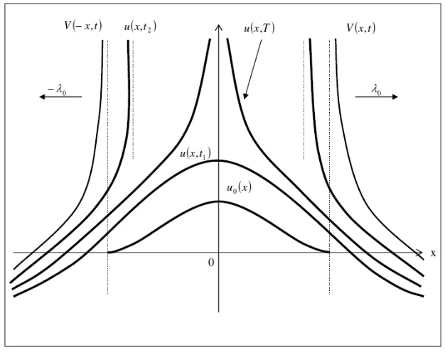
In general, quasilinear heat equation is a natural problem which is to find conditions for complete and incomplete blow-up in terms of the constitutive functions. In principle, the alternative will also depend on the initial data. It is clear that for flat initial data (u constant) blow-up is always flat, hence complete. ₀ Incomplete blow-up is an admitting of power source of Porous Medium Equation (PME). The incomplete blow-up has some properties to consider. But, in this study, only one of the properties will be discussed.

The nonnegative solutions u=u(x, t) of the quasilinear heat equation

( )

xx m

t u u

371 An Improved Parallel AGE Method to Solve …

may blow up in finite time for some initial data u

( )

( )

2

1< p≤m+ solutions blow up for arbitrarily small initial datau₀, while for 2

+ >m

p blow up always occurs for sufficiently large initial function.

Let u(x, t) be the unique global proper (minimal) solution constructed by monotone increasing approximations, and T =T(u₀)be its finite blow up time. If the continuation of the solution beyond blow-up is trivial, i.e., u(x,t)≡∞ for t>T, we say that the blow-up is complete, otherwise, if u(x,t)≡∞ for t>T, it is incomplete.

The blow-up set B

[ ]

( )

[ ]

( )

{ }

{ }

B { : _k , _k withu(x_k,t_k)→∞}, (2)

and in the case of incomplete blow-up B

[ ]

( )

[ ]

1.2

The application to industry

Incomplete blow-up is one of a special Porous Medium Equation (PME) with power source. In industrial world, the porous medium is used as one of the process such as in the filtration process.

As we can see, filtration is the process of passing a flow containing suspended solids through a porous medium, the fabric. It has been widely accepted as an effective, reliable and economic method for solid-liquid separation. Some critical applications include sterilization of pharmaceutical fluids; control of sub micron contaminants is deionized water for integrated circuit manufacture and purification of a variety of chemicals and solvents. Greater performance demands are being placed on filtration systems with particular reference to increase security, improved economy and enhanced removal efficiency. A good knowledge of the technique is, therefore, essential for the process industry personnel.

For a number of reasons, the medical and laboratory product industries cannot rely solely on the current forms of filtration and separations materials for a new application.

The incomplete blow up Heat Equation (HE) will be discretized by using Partial Differential Equation (PDE) in this study. This discretization must be done to see whether the function is satisfying or not the condition that have been stated.

The key purpose on this study is to implement the new variance of AGE method. The accuracy of the AGE method is comparable. This method also employs the fractional splitting strategy and the implicit form. The second endeavor is to run the AGE method with the HPC platform. Through the Linux Programming, the algorithms of the AGE method will be coded and run by the HPC.

The final target is to analyze the equation. This step is important because there will be an example that can be run to find the error residual. The error will be compared through two methods which are Gauss-Seidel method and AGE method. The best method which can give the lowest error is the best method.

373 An Improved Parallel AGE Method to Solve …

which is used as a communication platform will be discussed in this section. The discretization of the incomplete blow-up and the performance analysis of Gauss Seidel and AGE programming will be discussed and the result will be compared in order to evaluate the performance in section 4. Finally, Section 5 will conclude the paper.

2.0 Numerical

Method under Consideration

There are two methods that have taken under consideration for this study which are the Alternating Group Explicit Scheme (AGE) method and the Gauss-Seidel method in solving the equation.

2.1

Alternating Group Explicit Scheme (AGE) Method

Through the Alternating Direction Implicit (ADI), Alternating Group Explicit Scheme (AGE) methods with Peaceman-Rachford variation are created to be more extremely powerful, flexible and these offer users many advantages. The accuracy of these methods are comparable if not better than that of the GE class of problem as well as other existing schemes presented by Evans and Abdullah [8]. These methods employ the fractional splitting strategy and the implicit form is as follows,

(

) (

[

)

]

2 1

1 2 1

f u G rI rI G

u⎜_⎝⎛ +k ⎟_⎠⎞ _{= +} − ₋ k ₊

(3)

( )

₍

_{) (}

₎

1

1 1

2 1

⎥ ⎥ ⎦ ⎤ ⎢

⎢ ⎣ ⎡

+ −

+

= ⎟⎠

⎞ ⎜ ⎝ ⎛ + −

+ _{G rI rI G u f}

u k k ₍₄₎

We have

.

2 1 G

G

A= + (5) if we resume m to be odd then Gˆ could be written as,

, ˆ

2 2 2 2

×

⎥ ⎦ ⎤ ⎢

⎣ ⎡

r c

b r

G (6)

where .

2 2

a r

r = + The alternating implicit nature of the (2×2) groups where the

implicit and explicit values are given on the forward and backward levels for

sweeps on the

th

k ⎟ ⎠ ⎞ ⎜ ⎝ ⎛ +

2 1

and

(

)

2 ,

2 2

1

a r r a r

r = − = + end

bc r − =

∆ 2

2 , k=1,2,…,n,

i. at the

th

k ⎟ ⎠ ⎞ ⎜ ⎝ ⎛ +

2 1

, 2 1 ) ( 2 ) ( 1 1 2 1 1 r f bu u r u k k

k − +

= ⎟ ⎠ ⎞ ⎜ ⎝ ⎛ + (7) , ) ( 2 ) ( 1 ) ( ) ( 1 2 1 ∆ + + + + = − + + ⎟ ⎠ ⎞ ⎜ ⎝ ⎛ + i k i k i k i k i k i E Du Cu Bu Au

u (8)

, ) ( 2 ) ( 1 ) ( ) ( 1 2 1 1 _∆ + + + + = − + + ⎟ ⎠ ⎞ ⎜ ⎝ ⎛ + + i k i k i k i k i k i E Du Cu Bu Au

u (9)

with i=2,4,6,…..,m-1, ⎪⎭ ⎪ ⎬ ⎫ ⎩ ⎨ ⎧ − ≠ − = = − = − = = − = + 1 , 1 , 0 , , , 2 1 2 1 2 1 2 m i b m i D bf f r E br C r r B cr A i i i (10) and ⎪⎭ ⎪ ⎬ ⎫ ⎩ ⎨ ⎧ − ≠ − − = = − = − = = − =

+ _{, 1}

1 , 0 , , , 2 1 2 1 2 1 2 m i b m i D bf f r E br C r r B cr A i i i 11)

ii. at the

(

)

( ) 2) _,

1 ( 2 ) 2 1 ( 1 ) 2 1 ( ) 2 1 ( 1 1 ∆ + + + + = + + + + + + − + i k i k i k i k i k i T Su Ru Qu Pu

u (12)

( ) 2( ) _,

) ( 1 ) ( ) ( 1 1 1 _∆ + + + + = − + + + + i k i k i k i k i k i T Su Ru Qu Pu

u (13)

( ) 2) _,

1 ( 1 ) 2 1 ( 1 1 ∆ + + − = − + + + m k m k m k m f u r cu

u (14)

With ⎪⎭ ⎪ ⎬ ⎫ ⎩ ⎨ ⎧ ≠ = = − = = − = =

+ _{, 1}

1 , 0 , , , , 2 1 2 2 1 2 1 i c i P bf f r T b S br R r r Q i i i (15) and ⎭ ⎬ ⎫ + − = − = = = − = + , _ , , , 1 2 2 2 1 2 i i

i cf r f

T br S r r Q R cr Q (16)

375 An Improved Parallel AGE Method to Solve …

IADE_BRIAN and IADE_DOUGLAS for one dimensional problem is presented in table 1 below.

Table 1: computational complexity for sequential IADE_BRIAN and IADE_DOUGLAS for one-dimensional problem

Methods Multiplication Addition

Constant of IADE_BRIAN IADE_BRIAN

18 10m + 5

7 8m + 5 Constant of IADE_DOUGLAS

IADE_DOUGLAS 21 12m + 7 11 8m + 5

Gauss Seidel Red Black 6m + 5 4m + 3

2.2 Gauss-Seidel

Method

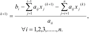
The Gauss-Seidel method attempts to solve the equations in a non-linear system within each period by a series of iterations which do not involve linear approximations. In the descriptions below the superscript represents the value calculated in the “n” th iteration and the superscript 0 indicates the starting value for the variable.

,

1 ) ( 1

1

) 1 (

) 1 (

ii n

i j

k j ij i

j

k j ij i

k i

a

x a x

a b

x

∑

∑

+ = −

=

+

+

− −

= (17)

. ,..., 3 , 2 ,

1 n

i= ∀

The Gauss-Seidel Method is more efficient than the Jacobi Method in terms of the rate of convergence.

2.3 The

Discretization

In previous sections, we have been overviewed the incomplete blow-up equation. In this subtopic, we will discuss the discretization of the incomplete blow-up equation. The incomplete blow-up is a two dimensional parabolic equation. From equation (1), we have

,

, ,

1

t

u

u

u

δ

−

=

(18)

, 2

)

( , 1 ₂, , 1

x u u u

um _xx i j ij ij

δ

+

− − +

= (19)

.

,j i p _u

The discretization is based on partial differential equation as shown below.

Substitute equation (18), (19), (20) into equation (1),

, 2 , 2 1 , , 1 , , , 1 j i j i j i j i j i j i u x u u u t u u + + − = − _{− +} + δ

δ (21)

(

)

1 , , 1 , 2 , ,

1j i j i j i j i j ij

i u u u x u

x t u u δ δ δ + + − = − _{− +}

+ (22)

Hence,

, 2

1 _{2 , 2 , 1}

1 , 2 ,

1 − +

+ ⎟ + ⎠ ⎞ ⎜ ⎝ ⎛ _{+ −} +

= _{ij ij i j}

j i u x t u x t t u x t u δ δ δ δ δ δ δ (23)

The equation (23) can be written in the matrix form:

⎣

⎦

[

]

where ⎟

⎠ ⎞ ⎜ ⎝ ⎛ − +

=1 2 ₂

x t t b δ δ

δ and ₂

x t c δ δ = .

2.4

Gauss Seidel Programming

The classical Gauss Seidel has been discussed in the previous section. The incomplete blow-up equation has been discrete according to the classical Gauss Seidel. The one dimensional incomplete blow-up:

, 2 2 p m u x u x

t _{= +} δ δ δ

δ

(25)

and the discretization of the form,

, 2 2 p m u x u x t + = δ δ δ δ (26) , 2 , 2 1 , , 1 , , , 1 j i j i j i j i j i j i u x u u u t u u + + − = − _{− +} + δ

δ (27)

Giving the explicit formula,

, 2

1 _{2 , 2 , 1}

1 , 2 ,

1 − +

+ ⎟ + ⎠ ⎞ ⎜ ⎝ ⎛ _{+ −} +

= _{i j i j ij}

377 An Improved Parallel AGE Method to Solve …

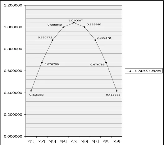
The Gauss Seidel programming has been done by using C Programming. The graph of the Gauss Seidel approximation can be seen in the Fig. 2.

From Fig. 2, we can see that the Gauss Seidel method gives the parabolic curve to the value of xi. The value of x1 = x9 =0.415383,x2=x8=0.676786, x3=x7=0.880472,

x4=x6=0.999940, and x5=1.040007. From the programming that has been run, the

number of iteration for Gauss Seidel method is 150 iterations with the error drop to 0.

Fig. 2: Gauss Seidel Approximation Graph

2.5

AGE Method Programming

The algorithm for the AGE method has been discussed in the previous section. This method employs the fractional splitting strategy and the implicit form is as follows,

(

) (

[

)

]

2 1

1 2 1

f u G rI rI G

u k ⎟⎠ _{= +} − ₋ k ₊

⎞ ⎜ ⎝ ⎛ +

(29)

( )

₍

_{) (}

₎

2 1 ( 1 1

2 1

⎥ ⎦ ⎤ ⎢

⎣ ⎡

+ −

+

= − +

+ _{G rI rI G u f}

u k k ₍₃₀₎

with k=1,2,…..,n and

.

2 1 G

G

A= + (31) By using AGE approximation, we got the result as in Fig. 3.

1.040007 0.999940

0.880472 0.880472

0.676786 0.676786

0.415383 0.415383 0.999940

0.000000 0.200000 0.400000 0.600000 0.800000 1.000000 1.200000

x[1] x[2] x[3] x[4] x[5] x[6] x[7] x[8] x[9]

Fig. 3: AGE Approximation Graph

From Fig. 3, we can see that the AGE method gives the parabolic curve to the value of xi. The value of x1 = x9 =0.415382,x2=x8=0.676786, x3=x7=0.880472,

x4=x6=0.999939, and x5=1.040007. From the programming that has been run, the

number of iteration for AGE method is 200 iterations with the error drop to 0.

3.0 Performance

Analysis

We can compare both Gauss Seidel and AGE approximation method to get the four important components which are convergent rate by the number of iteration, execution time, computational complexity and stability.

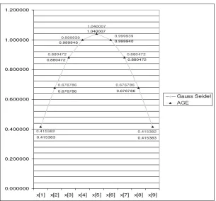
As we can see from Fig. 4, Gauss Seidel and AGE method got the parabolic curve which means that the both approximations are valid.

1.040007

0.999940 0.999940

0.880472 0.880472

0.676786 0.676786

0.415383 0.415383

0.000000 0.200000 0.400000 0.600000 0.800000 1.000000 1.200000

x[1] x[2] x[3] x[4] x[5] x[6] x[7] x[8] x[9]

379 An Improved Parallel AGE Method to Solve …

Fig. 4: Gauss Seidel and AGE Approximation Graph

From the Fig. 4, we cannot see any different between Gauss Seidel and AGE approximation. But by the value of each xi, we can see the different at x1 , x4 , x6

and x9. The different is 0.000001 at all point x1 , x4 , x6 and x9. From Table 2, we

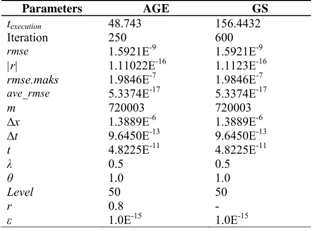
can see that the number of iteration for Gauss Seidel method is 600 and AGE method is 250 with the lower error rate that Gauss Seidel method. The rate of convergence of AGE is better than Gauss Seidel method. The degree of accuracy of AGE

method is higher than Gauss Seidel method. This proved by texecution (Execution time),

iteration and |r|=absolute errors, generated by AGE method have a lowest value than Gauss Seidel method. Table 3 shows the parallel computational complexity and communication cost for AGE and GS methods and here it’s shown that computational

complexity and communication cost of AGE are lower than GS method. Hence, it is

Table 2: Analysis of AGE_BRAIN and Gauss-Seidel methods

Parameters AGE GS

texecution 48.743 156.4432

Iteration 250 600

rmse 1.5921E-9 1.5921E-9

|r| 1.11022E-16 1.1123E-16

rmse.maks 1.9846E-7 _1.9846E-7

ave_rmse 5.3374E-17 5.3374E-17

m 720003 720003

∆x 1.3889E-6 1.3889E-6

∆t 9.6450E-13 9.6450E-13

t 4.8225E-11 4.8225E-11

λ 0.5 0.5

θ 1.0 1.0

Level 50 50

r 0.8 -

ε 1.0E-15 _1.0E-15

rmse=root mean square error, |r|=absolute error, r.maks=maximum error and ave_rmse=average of rmse

Table 3: Computational complexity and communication cost of AGE

Method Computational complexity communication cost AGE

D p

m T

p m

⎟⎟ ⎠ ⎞ ⎜⎜

⎝ ⎛

+ +

⎟⎟ ⎠ ⎞ ⎜⎜

⎝ ⎛

+1257 2250 1268

2250 3000tdata+1500(tstart+

tidle)

GS

D p

m T

p m

⎟⎟ ⎠ ⎞ ⎜⎜

⎝ ⎛

+ +

⎟⎟ ⎠ ⎞ ⎜⎜

⎝ ⎛

+1800 3600 3000

2400 7200tdata+3600(tstart+

tidle)

D=multiplication, T= addition

4.0 Parallel

Architectures

381 An Improved Parallel AGE Method to Solve …

environmental modeling, fluid dynamics simulations, and weather prediction applications.

PVM system is implemented on a hardware base which is consists of different machine architectures, including single CPU systems, vector machines, and multiprocessors. This computing element is interconnected by one or more networks, which may themselves be different like one implementation of PVM operates on Ethernet, Internet and a fiber optic network [9].

C, C++ and FORTRAN are all languages that can be used to write PVM codes. This project is done by using C languages by UNIX as an operating function. To execute an application, a user typically starts one copy on one task from a machine within the host pool.

Task-to-task communication in PVM is done with message passing. Message passing is a set of tasks that use their own local memory during computation. Multiple tasks can reside on the same physical machine as well as across an arbitrary number of machines. Tasks exchange data through communications by sending and receiving messages. Data transfer usually requires cooperative operations to be performed by each process. For example, a send operation must have a matching receive operation.

5.0 Performance Analysis of PVM

There are a master task and a number of worker tasks in the PVM implementation of the modeling codes. Master task is responsible to divide the model domain into sub domains and distribute them to worker tasks. Then, the workers tasks perform time marching and communicate after each time step. Time execution, speedup, efficiency, effectiveness and temporal performance will be analyzed by looking at the performance of the parallel algorithm.

Parallel Analyses of the basic PDE

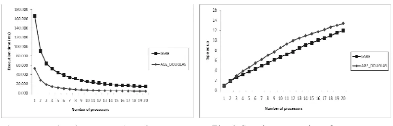
From Fig. 5,6,7,8 and 9, we can see that AGE method is providing better results than Gauss Seidel method on parallel environment in terms of time of execution, speedup, efficiency, effectiveness and temporal performance depending on the number of processors. One dimensional PDE was applied for this analysis.

Parallel Analyses to solve incomplete blow-up The Time Execution

The time execution has been determine when running the parallel algorithm. The result of the time execution is as below.

Table 4 and Fig. 10 shows the time execution of one dimensional parabolic equation model implemented to the parallel computing. The time execution has been determined by using two different method which are AGE and Gauss Seidel (GS) method. The size of the matrices; m=70000 has been used to see the time execution. The time execution of AGE method is lower than GS method for all number of processors. It means that AGE method is the better than GS method while running the incomplete blow-up parallel computing system.

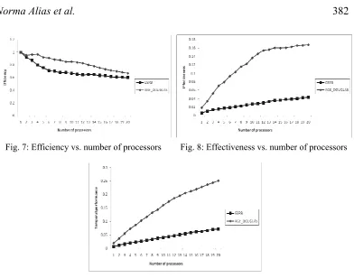
Fig. 7: Efficiency vs. number of processors Fig. 8: Effectiveness vs. number of processors

383 An Improved Parallel AGE Method to Solve …

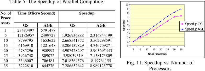
The Speedup

The Amdahl’s law state that the speed of a program is the time to execute the program while speedup is defined as the time it takes a program to execute in serial (with one processor) divided by the time it takes to execute in parallel (with many processors).

Table 5: The Speedup of Parallel Computing

No. of Proce

ssors

Time (Micro Second) Speedup

GS AGE GS AGE

1 23483497 5791478 1 1

5 12186957 2499727 1.926936888 2.316844199

10 8799795 1653622 2.668541372 3.502298591

15 6169910 1221648 3.806132829 4.740709271

20 4785296 980992 4.907428297 5.903695443

25 3926748 809072 5.98039319 7.158173809

30 3346007 706481 7.018364576 8.19764155

35 3222810 644276 7.286652642 8.989125778

Table 5 and Fig. 11 show that the speedup of parallel computing system while running the AGE and GS method. From Fig. 6, the speedup for both AGE and GS methods are increased. According to the Amdahl’s law, the speedup increases with the number of processors increase up to the certain level. For this problem, the speedup of the level from 15 to 35 processors increases slower than the speedup of lower number of processors. However, the parallel computing has been used to show that AGE method has higher than GS for the number of processors.

The Efficiency

The efficiency of a parallel algorithm is a measure of processor utilization. Efficiency is the speedup divided by the number of processors that has been used.

Number of Processors

Time (Micro Second) GS AGE

1 23483497 5791478

5 12186957 2499727

10 8799795 1653622

15 6169910 1221648

20 4785296 980992

25 3926748 809072

30 3346007 706581

35 3222810 644276

Fig. 11:Speedup vs. Number of Processors

0 1 2 3 4 5 6 7 8 9 10

1 5 10 15 20 25 30 35

No. of Processors

Spe

e

dup Speedup GS

Speedup AGE

0 5000000 10000000 15000000 20000000 25000000

1 5 10 15 20 25 30 35

No. of Processors

E

x

ec

ut

io

n Ti

m

e

Time (Micro Second) GS

Time (Micro Second) AGE

Table 4:The Time Execution of Parallel Computing

Table 6:The Efficiency of Parallel Computing

No. of Proce

ssors

Time (Micro Second) Efficient

GS AGE GS AGE

1 23483497 5791478 1 1

5 12186957 2499727 0.385387 0.463369

10 8799795 1653622 0.266864 0.350230

15 6169910 1221648 0.253742 0.316047

20 4785296 980992 0.245371 0.295185

25 3926748 809072 0.239216 0.286327

30 3346007 706481 0.233945 0.273255

35 3222810 644276 0.208190 0.256832

Table 6 shows that the efficiency decreases with the increasing of the number of processors, p. Poor load balance when imbalance workload distributed among the different processors is the factor that the decreasing of efficiency happened. It is also contributed by idle time, time startup and waiting for all processors to complete the computations. However, from the Fig. 12, the AGE method still more efficient method than GS method.

The Effectiveness

The effectiveness of the method by using parallel algorithm has been determined by calculate the speedup and efficiency.

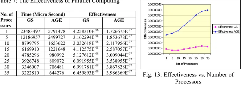
Table 7:The Effectiveness of Parallel Computing

No. of Proce ssors

Time (Micro Second) Effectiveness

GS AGE GS AGE

1 23483497 5791478 4.258310E-08 _1.726675E-07

5 12186957 2499727 3.162294E-08 _1.853678E-07

10 8799795 1653622 3.032618E-08 _2.117956E-07

15 6169910 1221648 4.112575E-08 _2.587057E-07

20 4785296 980992 5.127612E-08 _3.009044E-07

25 3926748 809072 6.091955E-08 _3.538955E-07

30 3346007 706481 6.991781E-08 _3.867828E-07

35 3222810 644276 6.459893E-08 _3.986369E-07

Table 7 and Fig. 13 show the effectiveness for both AGE and GS method by using parallel computing system. The formula of the effectiveness depending on the speedup; when speedup increases, the effectiveness is also increase. From the graph we noticed that the AGE method is more effective than GS method.

Fig. 12:Efficiency vs. Number of Processors

Fig. 13:Effectiveness vs. Number of Processors

0 0.2 0.4 0.6 0.8 1 1.2

1 5 10 15 20 25 30 35

No. of Processors

E

ff

ici

en

cy

Efficiency GS Efficiency AGE

0.00000000 0.00000005 0.00000010 0.00000015 0.00000020 0.00000025 0.00000030 0.00000035 0.00000040 0.00000045

1 5 10 15 20 25 30 35

No. of Processors

Ef

fe

c

ti

v

enes

s

385 An Improved Parallel AGE Method to Solve …

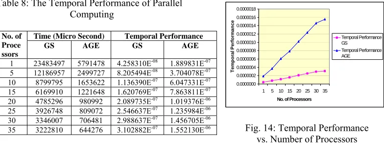
The Temporal Performance

Temporal performance is a parameter to measure the performance of a parallel algorithm which is

Temporal=1/Time (p)

Where Time P = time execution using p processor.

Table 8:The Temporal Performance of Parallel Computing

No. of Proce ssors

Time (Micro Second) Temporal Performance

GS AGE GS AGE

1 23483497 5791478 4.258310E-08 _1.889831E-07

5 12186957 2499727 8.205494E-08 _3.704078E-07

10 8799795 1653622 1.136390E-07 _6.047331E-07

15 6169910 1221648 1.620769E-07 _7.863811E-07

20 4785296 980992 2.089735E-07 _1.019376E-06

25 3926748 809072 2.546637E-07 _1.235984E-06

30 3346007 706481 2.988637E-07 _1.456705E-06

35 3222810 644276 3.102882E-07 _1.552130E-06

The temporal performance of parallel computing of AGE and GS method can be determined from Fig. 14. The Fig. shows increasing temporal performance for both methods. As showed above, the AGE method has higher temporal performance than GS method.

5.1 Granularity

Migration from sequential to parallel promises the existence of communication between working processors. Thus, the execution time measured for parallel implementation will be totally different with sequential. Parallel execution time will consider the time consumed for computation as well as time consumed for communication process. Communication cost involves time spent during sending and receiving messages. As computation and communication can be separately measured, granularity can be taken into account parallel performance evaluation. In [10], Kwiatkowski defines granularity as

comm comp

T T G =

Where T_comp and T_comm each represents computation and communication time. By measuring granularity, the ratio between computations to communication time can be explicitly shown. High rate of granularity shows that computation time holds the higher percentage out of overall execution time.

Fig. 14: Temporal Performance vs. Number of Processors

0.0000000 0.0000002 0.0000004 0.0000006 0.0000008 0.0000010 0.0000012 0.0000014 0.0000016 0.0000018

1 5 10 15 20 25 30 35

No. of Processors

Te

m

por

a

l Pe

rf

or

m

a

nc

e

Temporal Performance GS

Table 9x: Granularity Rate, Percentage of Execution, Communication, and Computation Time for Solution Using GS method

p Execution time Computation time Granularity Communication time

Gauss Seidel

5 44.10 30.99 2.36 13.11

% 70.27 29.73

10 24.88 16.04 1.82 8.831

% 64.47 35.49

15 17.19 10.33 1.51 6.856

60.09 39.88

20 13.90 7.822 1.29 6.078

% 56.26 43.72

Table 9y: Granularity Rate, Percentage of Execution, Communication, and Computation Time for Solution Using AGE method

p Execution time Computation time Granularity Communication time

AGE

5 11.00 9.60 6.9 1.40

% 87,27 12.72

10 5.85 4.72 4.2 1.12

% 80.68 19.14

15 4.35 3.18 2.7 1.16

73.10 36.47

20 3.62 2.39 1.9 1.23

% 66.02 51.46

387 An Improved Parallel AGE Method to Solve …

Granularity

0 1 2 3 4 5 6 7 8

5 10 15 20

No. of Processors

G

ran

u

la

ri

ty Ra

te

Granularity GS Granularity AGE

Efficiency vs Num ber of Process ors

0 0.1 0.2 0.3 0.4 0.5 0.6 0.7 0.8 0.9 1

5 10 15 20

No. of Processors

E

ff

ici

en

cy Rat

e

Ef f iciency GS

Ef f iciency AGE

This evaluation of granularity will be use in measuring parallel efficiency as stated by J. Kwiatkowski [10] where

1 1

1 1

+ = + =

G G

G E

This formula had been used to calculate the rate of efficiency and the result is as shown in Fig. 16. It shows the comparison of efficiency rate for problem solution using GS and AGE method. AGE donates better efficiency rate compared to GS and this shows the benefit of AGE method’s usage in computation.

6.0

Conclusions and Open Problems

Porous Medium Equation (PME) has been adopted in one of the important process in the industry that is the filtration process. In recent years, this filtration process is very important to the industry especially in medical and laboratory application. In 1950, Zel’dovich and coworkers developed the heat radiation in plasma by using the PME [11, 12]. Other applications that have been proposed is in mathematical biology, spread of viscous fluids, boundary layer theory, and other fields.

Though, it is still an open problem to discover conditions for complete and incomplete blow-up in terms of the constitutive functions by quasilinear heat equation, in this study, one of the properties (i.e., incomplete blow-up) under PME has been chosen to be solved by using the AGE method. The properties have been stated in the book written by Victor A. Galaktionov [13]. This parabolic equation described the first properties in incomplete blow-up that may blow-up in finite time u

( )

The mathematical problem in this study is solved by using the HPC system with PVM. The performance analysis of PVM has been done and the five terms which are time execution, speedup, efficiency, effectiveness and temporal performance has been determined. Both AGE and Gauss Seidel method has been compared when determined the graph of each terms. The HPC has been used to run a large scale problem.

At the beginning the parabolic equation incomplete blow-up has been solved by the Gauss Seidel and a new variance of the AGE method. Both equations have been run using C programming to see whether Gauss Seidel or AGE method is the best algorithm to solve the equation by comparing their convergence rate. From that analysis, it’s proved that AGE is the best algorithm to solve the parabolic equation incomplete blow-up.

ACKNOWLEDGEMENT

The authors wish to state their appreciation and thanks to the Technology University of Malaysia and the Malaysian government for providing the moral and financial support under the e-Science Research grants (Grant No. 72019) forth-successful completion of this project.

REFFERENCES

[1] Galaktionov, V.A. “Five types of blow-up in a semilinear Fourth-order reaction-diffusion equation: An analytic-numerical approach”, Nonlinearity, 22(7), (2009), pp. 1695-1741.

[2] Noriko Mizoguchi, “Multiple blowup of solutions for a semilinear heat equation”, Mathematische Annalen, 331, (2005), pp. 461–473.

[3] Natalini, R., Sinestrari, C. and Tesei, A. “Incomplete Blowup of Solutions of Quasilinear Hyperbolic Balance Laws”, Arch. Rational Mech, Anal. (Springer-Verlag), 135, (1996), pp 259-296.

[4] José M. Arrieta and Aníbal Rodríguez-Bernal, “Localization on the Boundary of Blow-up for Reaction–Diffusion Equations with Nonlinear Boundary Conditions”, Communications in Partial Differential Equations, 29(7&8), (2004), pp 1127–1148.

[5] Noriko Mizoguchi and Juan Luis Vazquez, “Multiple blow-ups for semilinear heat equations at different places and different times”, Indiana University mathematics journal, 56(6), (2007), pp 2859-2886.

389 An Improved Parallel AGE Method to Solve …

[7] Catherine A. Roberts, “Recent results on blow-up and quenching for nonlinear Volterra equations”, Journal of Computational and Applied Mathematics, 205, (2007), pp 736 – 743.

[8] Evans, D. J. and Abdullah, A. R. B. “Group Explicit Method for Parabolic Equations [J]”, Inter. J. Comput. Math., 14, (1983), pp 73-105. [9] Sunderam, V. S., and Geist, G. A. “The PVM System: Supercomputer

Level Concurrent Computation on a Network of IBM RS/6000 Powerstations”, Proceedings of the Large Scale Analysis and Modeling Conference, Park City, UT, (1991), pp 258-261.

[10] Jan Kwiatkowski, “Evaluation of Parallel Programs by Measurement of Its Granularity”, In Parallel Processing and Applied Mathematics, R. Wyrzykowski et al., Eds., (2002), pp 145–153, Springer-Verlag Berlin Heidelberg,.

[11] Ko, Y. “Regularity of the interface for the porous medium equation”, Electron. J. Differential Equations, 68, (2000), pp 1-12.

[12] Ya. B. Zel’dovich, and Kompaneets, A.S. “Towards a theory of heat conduction with thermal conductivity depending on the temperature”, in Collection of papers dedicated to 70th Anniversary of A. F. Ioffe, Izd. Akad. Nauk SSSR, Moscow, (1950), pp 61-72.