Accurate Gradient Computation for Elliptic Interface Problems with Discontinuous and Variable Coefficients

(1)

ABSTRACT

CHEN, GUANYU. Accurate Gradient Computation for Elliptic Interface Problems with Discontinuous and Variable Coefficients. (Under the direction of Dr. Zhilin Li.)

(2)

(3)

Accurate Gradient Computation for Elliptic Interface Problems with Discontinuous and Variable Coefficients

by Guanyu Chen

A dissertation submitted to the Graduate Faculty of North Carolina State University

in partial fulfillment of the requirements for the Degree of

Doctor of Philosophy

Applied Mathematics

Raleigh, North Carolina 2015

APPROVED BY:

Dr. Alina Chertock Dr. Ernest Stitzinger

Dr. Xiaobiao Lin Dr. Zhilin Li

(4)

DEDICATION

To my wife, Yan Li

To my parents, Jian Chen and Ping Wang

(5)

BIOGRAPHY

(6)

ACKNOWLEDGEMENTS

It is my honor to thank the many people who have helped me through this work. I would like to express my deepest gratitude to my advisor and mentor, Dr. Zhilin Li, for his guidance, training and support throughout my PhD study. These last five years have been amazing for me. I have been able to grow as a student, and more importantly, as a man. He not only taught me the knowledge needed to be successful in research but also led by example the correct attitude towards challenges on our way. His enthusiasm, meticulousness and great patience helped me continuously to accomplish in my research work. The experience I learned from his guidance will be an invaluable part of my life.

I would like to thank my committee members, Dr. Alina Chertock, Dr. Ernest Stitzinger and Dr. Xiaobiao Lin for reviewing my dissertation and offering valuable suggestions. I would also like to thank Mrs. Denise Seabrooks for her kind help during my six years in the graduate program.

I also want to thank Haifeng Ji and Professor Jinru Chen from Nanjing Normal University for their collaborations and discussions on my research. Thanks also go to my dear friends at NC State University for their help and collaborations on the research projects: Peng Song, Sidong Zhang, Zhaohui Wang, Tom and Mami Wentworth, Paige Shy, Ralph Abbey, Katherine Varga, Ming Jiang, Min Yang, Anna Fregosi, Gadi Elamami and Ranya Ali.

(7)

LIST OF TABLES

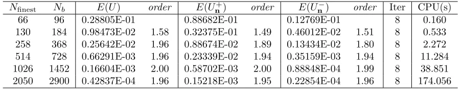
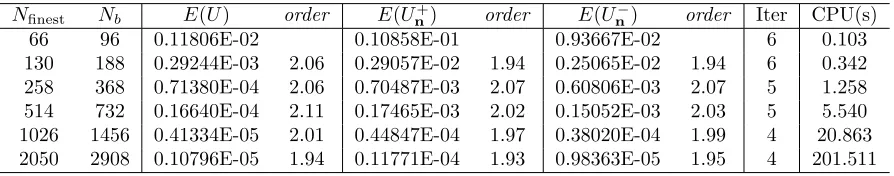
Table 4.1 Numerical results and convergence analysis for Example 4.1.1,Ncoarse= 5. 66

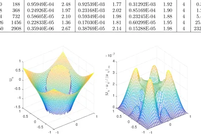
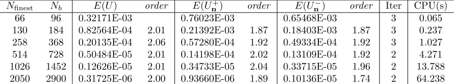
Table 4.2 Numerical results and convergence analysis for Example 4.1.2,Ncoarse= 5. 68

Table 4.3 Numerical results and convergence analysis for Example 4.2.1,Ncoarse =

5, C = 0.1, b= 0.05. . . 69 Table 4.4 Numerical results and convergence analysis for Example 4.2.1,Ncoarse =

5, C = 0.1, b= 3.5. . . 70 Table 4.5 Numerical results and convergence analysis for Example 4.4.1,Ncoarse =

5. . . 74 Table 4.6 Numerical results and convergence analysis for Example 4.5.1,Ncoarse =

(10)

LIST OF FIGURES

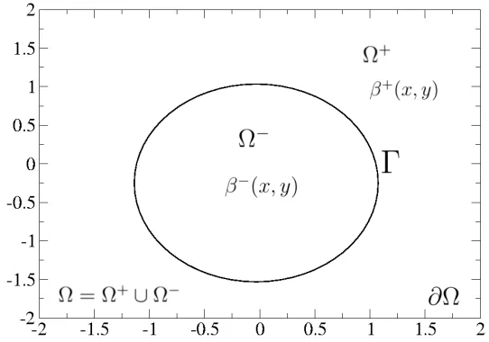
Figure 1.1 A typical rectangular domain Ω = Ω+_∪_Ω− _{with an interface Γ. The} coefficients β(x) have a finite jump across the interface Γ. . . 3 Figure 2.1 A diagram of the local coordinates in the normal and tangential

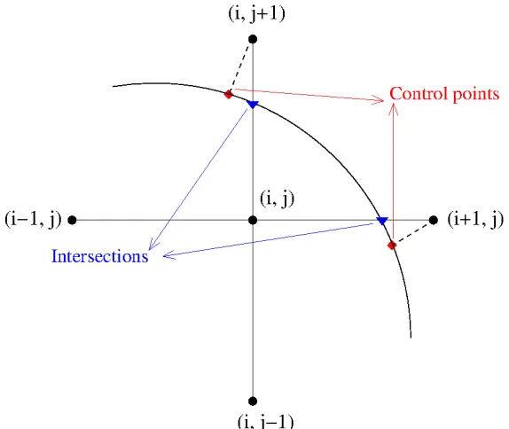
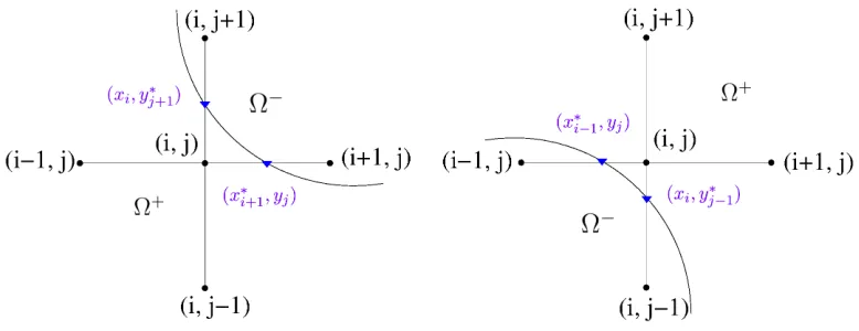
direc-tions, where θ is the angle between the x-axis and the normal direction. 27 Figure 2.2 The geometry at an irregular grid point (xi, yj). The red diamonds are

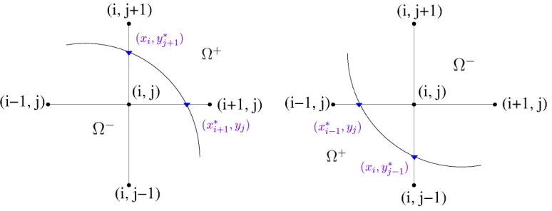
the control points, which are the orthogonal projections of the grid points (xi, yj+1) and (xi+1, yj) on the interface. The blue triangles are the intersection points, where the interface intersects with the grid lines involved in the 5-point stencil. . . 33 Figure 2.3 The irregular grid point (xi, yj) in the Ω−subdomain. At least one of its

four nearest neighbor grid points must belong to the other subdomain Ω+. The intersections are labeled by the little blue triangles, with their coordinates listed inside the parentheses. . . 34 Figure 2.4 The irregular grid point (xi, yj) in Ω+ subdomain. At least one of its

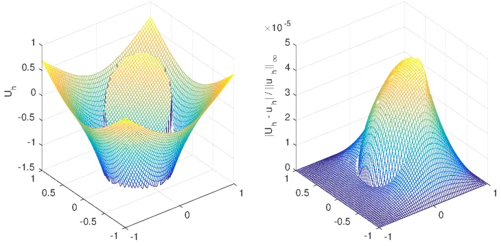
four nearest neighbor grid points must belong to the other subdomain Ω−. The intersections are labeled by the little blue triangles, with their coordinates listed inside the parentheses. . . 35 Figure 4.1 The computed solution and the distribution of the relative error for

Example 4.1.1. . . 67 Figure 4.2 The computed solution and the distribution of the relative error of

Example 4.1.2. . . 68 Figure 4.3 The computed solution and the distribution of the relative error of

Example 4.2.1, with C = 0.1, b= 3.5. . . 70 Figure 4.4 The computed solution and the distribution of the relative error of

Example 4.2.1, with C = 0.1, b= 0.05. . . 71 Figure 4.5 The number of GMRES iterations versus the number of grid lines N

in the x-direction. . . 72 Figure 4.6 The number of GMRES iterations versus the ratio of jumps β−/β+ _in

the log-log scale for Example 4.2.1 with a fixed mesh size M = 130 and N = 130. . . 73 Figure 4.7 The computed solution and the distribution of the relative error for

Example 4.4.1. . . 74 Figure 4.8 The computed solution and the distribution of the relative error for

Example 4.5.1. . . 82 Figure 4.9 The computed solution and the distribution of the relative error for

(11)

(12)

Chapter 1

Introduction

1.1

Interface problems

1.1.1

Applications of interface problems

(13)

or two states, and the source terms are often singular. As a result, the solutions to the differential equations are typically nonsmooth, or even discontinuous across the interface. Therefore, many standard numerical methods based on the assumption of smoothness of solutions do not work or work poorly for interface problems, due to the complications arise from the presence of interfaces, discontinuities in the coefficients and the singular source terms.

To develop numerical methods for interface problems, the main challenges lie in how to obtain an approximate solution with certain order of accuracy near or on the interface and how to efficiently solve the linear system of equations involved. Our work in this dissertation is also centered around these two key questions.

1.1.2

Elliptic PDEs with interfaces

In this dissertation, we’re interested in elliptic interface problems. An elliptic interface problem can be written in the following form,

∇ · β(x, y)∇u(x, y)

+σ(x, y)u(x, y) =f(x, y), (x, y)∈Ω = Ω+∪Ω−, (1.1)

together with the jump conditions across the interface Γ ,

[u]Γ=w, [βun]Γ=v, (1.2)

where Ω is a rectangular domain with a prescribed boundary condition on ∂Ω and β ≥

βmin > 0. Within this domain, Γ is an interface between two subdomains Ω+ and Ω−,

across which, the diffusion coefficientβis discontinuous, see Figure 1.1 for an illustration.

un is the normal derivative on the interface, which is defined asun =

∂u

(14)

n is the normal direction of the interface Γ pointing outward. Moreover, the coefficient

β(x, y) is variable in each subdomain,

β(x, y) =

      

β+₍_{x, y}₎ _{if (}_{x, y}₎_∈_Ω+_, β−(x, y) if (x, y)∈Ω−.

(1.3)

The functions w and v are two jump conditions defined only along the interface Γ. σ

and f are piecewise continuous functions, i.e.,σ±(x, y)∈C,f±(x, y)∈C, but may have a finite jump discontinuity across the interface. The interface Γ is assumed to be twice continuously differentiable along the interface, i.e., Γ ∈ C2_{. The solution is assumed to}

be twice continuously differentiable in each subdomain, i.e.,u±(x, y)∈C2_{. The diffusion}

coefficient β(x, y) is assumed to be continuously differentiable in each subdomain, i.e.,

β±(x, y)∈C1_.

(15)

The jump conditions across the interface Γ are defined as:

[u]Γ def

=u+ X(s), Y(s)−u− X(s), Y(s) =w(s), (1.4) [βun]Γ

def

=β+ X(s), Y(s)u+_n X(s), Y(s)

−β− X(s), Y(s)u−_n X(s), Y(s)=v(s),

(1.5)

where X(s), Y(s) is the arc-length parametrization of the interface Γ. The + and −

signs are assigned to be the limiting values of a function taken from the subdomain Ω+ and the subdomain Ω−.

Note that if the first jump condition [u] =w= 0, the solution to the interface problem (1.1) is equivalent to the solution of the following equation in the entire domain including the interface (Ω+_∪_Ω−_∪_{Γ), with a singular source on the right hand side,}

∇ · β(x, y)∇u(x, y)+σ(x, y)u(x, y) =f(x, y) +

Z

Γ

v(s)δ(x−X(s))ds . (1.6)

whereδis the two-dimensional Dirac-delta function. The second jump condition [βun] =v

can then be derived by integrating the above equation,

lim

Ω0→0

Z Z

Ω0

∇ · β(x)∇u(x)+σ(x)u(x)−f(x)−

Z

Γ

v(s)δ(x−X(s))ds dx= 0 =⇒

Z

Γ

β+(x)∇u+(x)·n− β−(x)∇u−(x)·n−v(s) ds= 0 =⇒[βun]Γ =v(s)

(1.7)

where Ω0 is a small integration domain that contains the entire interface Γ. The second

(16)

of delta function. Note that the normal derivativeun is usually discontinuous across the

interface due to the discontinuity in the coefficient β. And if w6= 0, the solutionu itself would also be discontinuous across the interface.

1.2

A review of numerical methods for elliptic

inter-face problems

There are many applications in solving elliptic equations with discontinuous coefficients, for example, steady state heat diffusion, multi-phase flow, crystallization process, and bubble simulation, and etc. Moreover, solving one or several elliptic interface problems is also the most expensive step of several well-known efficient methods for Navier-Stokes equations. There are two main concerns in solving (1.1)–(1.3). The first concern is about how to discretize (1.1)–(1.3) accurately. It is difficult to study the consistency and the stability of a numerical scheme because of the discontinuities across the interface. The second concern is about how to solve the resulting linear systems efficiently and robustly. Usually if the jump in the coefficient is large, the resulting linear system is ill-conditioned, and the number of iterations needed in solving such a linear system is large. That’s because the number of iterations usually is proportional to the jump in the coefficient.

(17)

1. The smoothing method

The idea of the smoothing method is to replace the original discontinuous coefficient

β(x) with a smoothing functionβ. We illustrate the idea through a one-dimensional example. Assume the coefficient β(x) has a finite jump at x = α, i.e., [β]α =

lim

x→α+β(x)−_x→αlim−β(x)6= 0.

We define a smoothing function β as

β(x) = ¯β−(x) + ( ¯β+(x)−β¯−(x))H(x−a), (1.8)

where ¯β+(x) and ¯β−(x) are continuously differentiable functions given by

¯

β−(x) =

      

β(x) if x≤α,

β(α−) +β0(α−)(x−α) if x > α,

(1.9a)

¯

β+(x) =

      

β(α+) +β0(α+)(x−α) if x < α,

β(x) if x≥α.

(1.9b)

H(x) is the smoothed Heaviside function,

H(x) =

              

0 if x≤ −,

1 2 1 +

x + 1 π sin πx

if |x| ≤,

1 if x > .

(1.10)

(18)

It is easy to implement the smoothing method in 1D, 2D and 3D if the interface is represented by the zero level set of a Lipschitz continuous function. The smoothing method is not very accurate because it smoothens the coefficientβ in the interface, as as result, the solution is also smoothened in the interface.

2. The harmonic averaging method

The harmonic averaging method [3, 25, 28] is more accurate than the smoothing method for discontinuous coefficients. Consider the one-dimensional model problem (βux)x =f(x), which can be discretized as

1

h2

β_i₊1

2(ui+1−ui)−βi− 1

2(ui−ui−1)

=f(xi), (1.11)

whereh=xi−xi+1 is the uniform grid spacing in thex-direction. For smooth β in

(xi−1, xi+1), we can takeβi+1₂ =β(xi+1₂), wherexi+1₂ =xi+

h

2, and the discretization is second-order accurate. But ifβis discontinuous in (xi−1, xi+1), then the harmonic

average of β(x) is

β_i₊1

2 =

1

h

Z xi+1

xi

β−1(x)dx

−1

. (1.12)

The finite difference scheme (1.11) using the harmonic averaging (1.12) is second order accurate in the infinity norm L∞ for 1D elliptic interface problems with [u]α = [βux]α = [f]α= 0, mainly due to the cancellation of errors.

(19)

3. Peskin’s immersed boundary (IB) method

To simulate the blood flow pattern in human’s heart, Peskin first developed the im-mersed boundary (IB) method [21, 22, 23, 20], which used numerical approximation of the δ function for singular sources on the interface.

There are several discrete delta functions in the literatures. The commonly used ones include the hat function

δ(x) =

    

(− |x|)

if |x|< ,

0 if |x|≥.

(1.13)

and Peskin’s original discrete cosine delta function

δ(x) =

    

1 4

1 + cosπx 2

if |x|<2,

0 if |x|≥2.

(1.14)

These two discrete delta function are both continuous. The second one, first in-troduced by Peskin and most often used in the literature, is also continuously differentiable.

It is easy to implement the IB method. In high dimensions, the discrete delta function is the product of one-dimensional discrete delta functions, for example, in 2D, δ(x, y) = δ(x)δ(y). With Peskin’s discrete delta function approach, we can discretize the right hand side of (1.6) at a grid point (xi, yj) as

Fij =fij + m

X

k=1

v(sk)δh(xi−Xk)δh(yj −Yk)∆s, (1.15)

(20)

h is the mesh spacing. Note that, from (1.13) and (1.14), we see that the singular source is distributed to grid points near the interface Γ.

The IB method is difficult to achieve high order accuracy. It is still a smoothing method that smears discontinuities. Using the IB method, we can achieve second order accurate solution in an average norm such as the L1 norm or the L2 norm. But it is unlikely to achieve a second-order accurate solution in the point-wise

L∞ norm. The reason is that the discrete right-hand size (1.15) is independent of the derivative of v(s) and the curvature of the interface, which are crucial in the immersed interface method (IIM) [7, 10] which we will discuss later in section 1.3.

4. Numerical methods based on integral equations

A. Mayo and A. Greenbaum [18, 19] have derived an integral equation for ellip-tic interface problems with piecewise constant coefficients. By solving the integral equation, they can obtain second-order accurate solutions in the L∞ norm using the techniques developed by Mayo in [16, 18] for solving Poisson and biharmonic equations on irregular domains. The total cost includes solving the integral equa-tion and a regular Poisson equaequa-tion. They also menequa-tioned the possibility to extend the method to variable coefficients in [18]. While this methods based on integral equations are very effective for homogeneous source terms, they usually require extra efforts for non-homogeneous source terms and different boundary conditions, for which the implementations of these methods are not trial.

(21)

in the point-wiseL∞norm. However, when dealing with interface problems, we are more interested in errors in the point-wiseL∞ norm instead of an averageL1 _or _L2 _{norm. An}

average norm cannot correctly reflect errors near the interface, while the point-wise L∞

norm usually reflects the accuracy of solutions near interfaces that are the main interest for many interface problems.

In the section below, we will introduce the immersed interface method (IIM) [7, 10], in which the discontinuities and the jump conditions are enforced either exactly or approximately. The IIM generally has a second-order accuracy globally, which means the computed solution is second-order accurate in the point-wise L∞ norm.

1.3

The immersed interface method (IIM) and an

augmented strategy

The immersed interface method (IIM) [7, 10] is a different approach developed by R. J. LeVeque and Z. Li for discretizing elliptic problems with irregular interfaces , which can handle both discontinuous coefficients and singular sources. The main idea is to incorpo-rate the jump conditions into the finite difference scheme near the interface using Taylor expansion. This approach has also been applied to 3D elliptic equations [11], parabolic equations [12, 15, 17], hyperbolic wave equations with discontinuous coefficients [9], and the incompressible Stokes flow problems with moving interfaces [8].

1.3.1

The IIM for elliptic interface problems

(22)

the standard finite difference methods. while near or on the interface, the IIM modifies the finite different schemes to treat the irregularities. Since the dimension of the inter-faces is one dimension lower than that of the solution domain, the modifications do not significantly increase the computational costs.

Here we illustrate the main idea of IIM through a one-dimensional model problem

(βux)x =f, x∈(0, α)∪(α,1), (1.16a) [u]x=α = 0, [βux]x=α =v, (1.16b)

with specified boundary conditions of u(x) at x = 0 and x = 1. The function β(x) is discontinuous atx=α. While this model problem is quite simple, it illustrates the main ideas of the IIM.

For simplicity, we assume that f(x) is a continuous function and β is piecewise con-stant with a finite jump at the interface x = α. From the jump conditions (1.16b) and the equation (1.16a), we first obtain the following interface relations, which express the limiting values from the ”+” side ( x > α) in terms of those from the ”−” side (x < α),

u+=u−, u+_x = β −

β+u

− x +

v β+, u

+

xx =

β−u−_xx

β+ (1.17)

The algorithm of IIM for (1.16a)–(1.16b) is then outlined below.

1. We first generate a uniform Cartesian grid for the finite difference method,

xi =ih, i= 0,1,2, . . . , N (1.18)

(23)

α ≤xj+1. Then, the grid points xj and xj+1 are called irregular grid points, while

the other grid points are called regular grid points.

2. We then determine the finite difference scheme for regular grid points.

At a grid pointxi, xi 6=j, j+ 1, we use the standard 3-point central finite difference approximation

1

h2

β_i₊1

2(Ui+1−Ui)−βi− 1

2(Ui−Ui−1)

=fi (1.19)

with β_i₊1

2 =β(xi+ 1

2), fi =f(xi).

3. Next, we determine the finite difference scheme for the irregular grid points xj and

xj+1.

We determine the finite difference coefficients using the method of undetermined coefficients,

γj,1Uj−1 +γj,2Uj +γj,3Uj+1 =fj +Cj,

γj+1,1Uj +γj+1,2Uj+1+γj+1,3Uj+2 =fj+1+Cj+1.

(1.20)

We now illustrate the idea of the IIM about how to determine the finite difference coefficients γj,1,γj,2 and γj,3 in (1.20).

We want to minimize the magnitude of the local truncation error

Tj =γj,1u(xj−1) +γj,2u(xj) +γj,3u(xj+1)−f(xj)−Cj. (1.21)

The main idea is to use Taylor expansion to expand the solution u(xj−1), u(xj),

(24)

The Taylor expansion foru(xj+1) at α is given by

u(xj+1) =u+(α) + (xj+1−α)u+x(α) + 1

2(xj+1−α)

2_u+

xx(α) +O(h

3₎_.

and the Taylor expansions of u(xj−1) and u(xj) at α can be written as

u(xl) = u−(x) + (xl−α)u−x(α) + 1

2(xl−α)

2_u−

xx(α) +O(h

3₎_, _l ₌_j₋₁_{, j.}

Then we use the interface relations (1.17) and choose to wirteu+₍_α_),_u+

x(α),u+xx(α) in terms of u−(α), u−_x(α), u−_xx(α). So we have a new expression for the Taylor expansion ofu(xj+1):

u(xj+1) =u−(α) + (xj+1−α)

β−

β+u

− x(α) +

v β+

+1 2(x

2

j+1−α) 2β

−

β+u

−

xx(α) +O(h

3₎_.

Thus, we now put all these expansions back to the local truncation error (1.21) at

x=xj, and collect terms for u−(α), u−x(α), u −

xx(α) to get

Tj =γj,1u(xj−1) +γj,2u(xj) +γj,3u(xj+1)−f(xj)−Cj = (γj,1+γj,2+γj,3)u−(α) +γj,3(xj+1−α)

v β+

+

(xj−1−α)γj,1+ (xj −α)γj,2+ β−

β+(xj+1−α)γj,3

u−_x(α) +1

2

(xj−1−α)2γj,1+ (xj−α)2γj,2+ β−

β+(xj+1−α) 2_γ

j,3

u−_xx(α)

−f(α)− O(h)−Cj +O

max

1≤l≤3|γj,l|h 3_.

(1.22)

(25)

α from the “−” side, we obtain a system of equations for the coefficients {γj,k}:

              

γj,1+γj,2+γj,3 = 0,

(xj−1−α)γj,1+ (xj−α)γj,2+ β−

β+(xj+1−α)γj,3 = 0,

1

2(xj−1−α)

2_γ

j,1+

1

2(xj−α)

2_γ

j,2+

1 2

β−

β+(xj+1−α) 2_γ

j,3 =β−.

(1.23)

Once those {γj,k}’s have been computed, the correction term is set to

Cj =γj,3(xj+1−α) v

β+ , (1.24)

which matches the remaining leading terms in the local truncation error Tj above. Similarly, we can get the {γj+1,k}’s by considering the local truncation error Tj+1

atx=xj+1 and following the same procedure above.

4. We can solve the linear system of equations (1.19)–(1.20) for all grid points, which is a tridiagonal matrix, to get an approximate solution of u(x) at all grid points.

For 2D and 3D elliptic interface problems, we can use the same IIM algorithm to derive the finite difference scheme for the irregular points on or near the interface.

Since the IIM incorporates the discontinuities and the jump conditions on the inter-face, it can achieve second-order accuracy in the point-wise L∞ norm. The second order accuracy of the IIM has been confirmed by many numerical examples and theoretical analysis. Note that, while the solutions have second order accuracy globally at all grid points, the local truncation errors at grid points near the interface are usually O(h) (see (1.22) for example), which is one order lower than that at regular grid points (O(h2_)).

(26)

for 2D and 3D interface problems. So we can use standard iterative methods such as an SOR or the multigrid method [2, 4] to solve the linear system of equations efficiently. But in some numerical examples with large jumps in the coefficients β, the resulting linear system is usually ill-conditioned. So it takes many number of iterations in solving such a system. The immersed interface method may converge very slowly or fail to give accurate answers.

In the next section, we explain an augmented strategy which can be used to solve some interface problems with large jumps in the diffusion coefficient β(x, y).

1.3.2

An augmented iterative algorithm for the IIM

The idea of the augmented strategy for interface problems was originally proposed by Z. Li [13] for elliptic interface problems with piecewise constant coefficients.

The augmented strategies have at least two advantages. The first is that the aug-mented strategies allow us to utilize the existing fast solvers to get a faster algorithm compared to direct discretization. The second is that, for certain types of interface prob-lems, an augmented approach may be the only way to obtain an accurate algorithm. For instance, in the incompressible Stokes equations, the jump conditions for the pressure and the velocity are usually coupled together. The augmented approach enables us to separate the jump conditions so that the idea of the IIM can be applied.

In augmented strategies, some augmented variable g defined only on the interface is introduced. If the augmented variable is known, it is relatively easy to solve the original problem.

(27)

be constant in each subdomain,

β(x, y) =

      

β+ _{if (}_{x, y}₎_∈_Ω+_, β− if (x, y)∈Ω−.

(1.25)

With this piecewise constant coefficient, the original PDE in (1.1) with σ(x, y) = 0 can be preconditioned to a Poisson equation in each subdomain by dividing the constantβ+

in the Ω+ subdomain and dividing β− in the Ω− subdomain from the original problem. So it is natural to introduce the jump in the normal derivative [un] as the augmented

variable. Thus, we have an equivalent problem:

      

∇2_u₍_{x, y}_{) =} f(x, y)

β+ , if (x, y)∈Ω +_,

∇2_u₍_{x, y}_{) =} f(x, y)

β− , if (x, y)∈Ω −_,

(1.26a)

[u]Γ =w, [un]Γ =g, (1.26b)

with the same boundary condition on ∂Ω as in the original problem (1.1). The regularity of the new problem is the same as previously mentioned in Section 1.1.2, i.e.,f is piece-wise continuous, f±(x, y)∈ C; the interface Γ is twice continuously differentiable along the interface, Γ ∈ C2_{; and the solution} _u _{is piecewise twice continuously differentiable,} u±(x, y)∈C2.

Then we can discretize the corresponding Poisson equation using the standard five-point stencil with some modifications in the right hand side. The discrete form of (1.26a) obtained from the IIM can be written as

∇2

hUij =

fij

βij

(28)

where Cij is a correction term, which is zero at a regular grid points, and is non-zero at irregular grid points, and the ∇2

h is the discrete Laplacian operator

∇2

hUij =

Ui+1,j+Ui−1,j+Ui,j+1+Ui,j−1−4Ui,j

h2 . (1.28)

The correction term Cij at an irregular grid point (xi, yj) can be derived from the IIM and is given as

Cij =a2w+a12g0+ (a6+a12χ00)w0+a10w00

+na4+ (a8−a10)χ00

o

g+a8

nf

β

−w00o,

(1.29)

wherew,w0,w00,g, andg0 are evaluated at a set of control pointsX1,X2, . . . ,XNb on the

interface. These control points are usually the orthogonal projections of the irregular grid points onto the interface. The {ai}’s are given by (3.4) in Chapter 3, which depends on the finite difference coefficients of the 9-point stencil centered at (i, j) and the positions of the 9-point stencil relative to the interface. We will explain this in detail when we generalize the augmented strategies to PDEs with piecewise variable coefficients.

Let W = [W1, W2, . . . , WNb]

T _and _G _{= [}_G

1, G2, . . . , GNb]

T _{be the discrete values of} the jump conditions (1.26b) at the control points X1,X2, . . . ,XNb on the interface. Let

B(W,G) be a mapping from W = [W1, W2, . . . , WNb]

T _and _G _{= [}_G

1, G2, . . . , GNb]

T _to

Cij in (1.29). In discrete form, all the surface derivatives of the jump conditions can be obtained from a linear combination of the values of W and G at {Xk}. Therefore,

B(W,G) can be written as a linear function of W and G

(29)

where B and B1 are two matrices with real entries.

Therefore, (1.27) can be re-written as a matrix vector equation, which combines the approximate solution (denoted byU) to the original problem and the augmented variable G (discrete form ofg) together

AU+BG=F+B1W=defF1. (1.31)

whereAis the matrix form of the discrete Laplacian operator andFis the vector formed by{fij

βij}. In (1.31), for a given augmented variable G, we can solve for the approximate

solutionU. In Z. Li’s original paper, fast Poisson solvers are utilized in solving for Uto give a fast algorithm.

Equation (1.31) has two unknowns, Uand G. So we need another constraint to form the second equation. We use the flux jump condition [βun] =v as the constraint. Define

the residual vector of the flux jump condition at {Xk} as

R(G) = [βUn](G)−V=β+U+n −β

−

U−_n −V. (1.32)

We want to find aG∗such thatR(G∗) = 0, where the vectorsU+

n andU

−

n are the discrete

approximations of the normal derivatives u±_n at{Xk} from each side of the interface. For an approximate G, we can obtain the solution Uby solving (1.31). Then, we can interpolate {Uij} in a linear manner to getUn±(Xk) at the control points{Xk}, 1≤k ≤

(30)

coefficient β. Since the interpolation is linear, we can write

∂U±(G)

∂n =E

±

U+T±G+P±V+Q±W, (1.33)

whereE+, E−, T+,T−,P+,P−, Q+, Q− are some sparse matrices determined from the interpolation scheme. These matrices are used only for theoretical purposes but are not actually constructed in implementation. We need to choose a vectorGsuch that the flux jump conditionβ+_U+

n−β

−_U−

n =V is satisfied along the interface Γ. Therefore, we have

a second matrix-vector equation

EU+TG−PV−QW= 0. (1.34)

If we eliminate U from the matrix vector equations (1.31) and (1.34), we get the Schur complement system for the augmented variable,

(T −EA−1B)G=PV+QW−EA−1F1 def

=F2. (1.35)

This is an Nb ×Nb system for G, a much smaller linear system compared to the one for U. Therefore, we can use the GMRES [24] iterative methods to solve the Schur complement system for the augmented variable. The matrix vector multiplication in GMRES iteration includes two main steps: (1) solving the original problem (1.31) for a given augmented variable G; (2) finding the residual of the constraint (1.32) using the computed approximate solution from the given augmented variable.

(31)

iterations is reasonably small and is independent of both the jumps in the coefficients and the mesh size.

1.4

Motivation to generalize the augmented strategy

to variable coefficients

Despite of the great success of the augmented IIM for piecewise constant coefficients, this method has never been applied to solve the elliptic interface equations with piecewise variable coefficients.

Generally speaking, to develop an augmented algorithm for variable coefficients, we need to solve four major problems. Firstly, we need to develop a new finite difference scheme at the irregular points since the discrete laplacian operator no long works for variable coefficients. Secondly, as a result of the first problem, we cannot take advantage of the fast Poisson solver [27]. Instead, we need to utilize a multigrid solver [5, 1], which is comparable to a fast Poisson solver using an FFT. Thirdly, the interpolation scheme in Z. Li’s original paper only works for piecewise constant coefficients. So we need to develop a generalized weighted least squares interpolation scheme for variable coefficients β to compute the normal derivatives on the interface from a grid function Uij. The accuracy of this interpolation scheme is crucial for the success of the augmented algorithm. Last but not least, we need to propose an efficient new preconditioner to solve the Schur complement system since the original one proposed in Z. Li’s paper [13] converges very slowly for interface problems with piecewise variable coefficients.

(32)

a second order accurate solution, but also a second order accurate gradient for some types of interface problems.

The idea is based on the augmented IIM, also called the fast IIM developed for inter-face problems with piecewise constant coefficients, in which, second order convergence of the solution and the gradient is achieved. The key of the new method is to introduce the jump in the normal derivative of the solution as the augmented variable and re-write the interface problem as a Laplacian of the solution with lower order derivative terms near the interface. Thus we can get jump relations for second order derivatives using the aug-mented variable and the lower order derivative terms. The idea should be applicable for boundary value problems with irregular domains as well. An upwind type discretization is used for the finite difference discretization near or on the interface so that the negative of the discrete coefficient matrix is an M-matrix. A multigrid solver DMGD9V [5] is used to solve the linear system of equations and a GMRES iterative method is used to solve for the augmented variable. Numerical experiments and convergence proof are also provided to show that the new method archives second order accuracy not only in the solution, but also in its gradient in the point-wise L∞ norm.

This dissertation is organized as follows.

Chapter 2 describes how to use the augmented IIM strategy to construct all the components of the linear systems. In Chapter 2, we first precondition the original elliptic interface equation to get an equivalent problem, which we can develop an augmented iterative algorithm to solve. Next we derive for the interface relations from the jump conditions and the PDE. Then we use the augmented IIM idea to discretize the equivalent problem and derive the Schur complement system.

(33)

scheme to approximate the discrete normal derivatives U±_n from the grid function Uij. Next, we use the multigrid solver DMGD9V to solve the linear system of equations for U and a GMRES iterative method to solve for the augmented variable G. The we propose an efficient preconditioner for the Schur complement system, which accelerates the convergence of the GMRES iterations.

Chapter 4 shows some numerical experiments and analysis to demonstrate that this new method can achieve the second order accuracy not only in the solution itself, but also in its gradient. Moreover, we also demonstrate the efficiency and robustness of the new method by showing that the number of iterations is almost independent of the mesh size and the ratio of the jump in the coefficients β(x, y). At the end of this chapter, we also generalize our new method for elliptic interface problems with non-zero σ(x, y) and demonstrate that it can achieve second order accuracy in both the solution and the gradient for these more general cases.

(34)

Chapter 2

Elliptic Interface Problems with

Variable Coefficients

Consider the elliptic interface problem,

∇ · β(x, y)∇u(x, y)=f(x, y), (x, y)∈Ω+∪Ω−,

[u]Γ=w, [βun]Γ =v,

(2.1)

in a rectangular domain Ω with a prescribed boundary condition on∂Ω andβ ≥βmin >0.

Within this domain, Γ is an interface, across which the coefficient β is discontinuous, as illustrated in Figure 1.1. Moreover, the coefficientβ(x, y) is variable in each subdomain,

β(x, y) =

      

β+₍_{x, y}₎ _{if (}_{x, y}₎_∈_Ω+_, β−(x, y) if (x, y)∈Ω−.

(2.2)

(35)

Γ. The interface Γ may or may not align with an underlining Cartesian grid.

The regularity of this problem is the same as mentioned in Chapter 1, i.e., the interface Γ is assumed to be twice continuously differentiable, Γ ∈ C2_{; the right hand side} _f _is

assumed to be piecewise continuous in each subdomain, f±(x, y) ∈ C; the solution u is assumed to be piecewise twice continuously differentiable in each subdomain, u±(x, y)∈

C2; and the coefficient β is assumed to be piecewise continuously differentiable in each subdomain, β±(x, y)∈C1.

In this chapter, we first precondition (2.1) and (2.2) to get an equivalent problem and derive necessary interface relations from the equivalent problem. Then we use the IIM idea to discretize the equivalent problem and derive the Schur complement system.

2.1

The equivalent problem

The original elliptic interface problem is stated inProblem I,

Problem (I).

∇ · β(x, y)∇u(x, y)=f(x, y), x∈Ω = Ω+∪Ω−, (2.3a)

Give BC on∂Ω, (2.3b)

with jump conditions along the interface Γ specified as

[u]Γ=w(s), (2.4a)

[βun]Γ=v(s). (2.4b)

(36)

we are interested in solving a new problem as stated in Problem II.

Consider the solution set ug(x, y) of the following problem as a functional of g(s).

Problem (II).

∇2u+∇β

+₍_{x, y}₎

β+₍_{x, y}₎ · ∇u=

f(x, y)

β+₍_{x, y}₎, if x∈Ω +

, (2.5a)

∇2_u₊∇β

−₍_{x, y}₎

β−₍_{x, y}₎ · ∇u=

f(x, y)

β−₍_{x, y}₎, if x∈Ω −

, (2.5b)

Give BC on∂Ω, (2.5c)

with specified jump conditions along the interface Γ

[u]Γ =w(s), (2.6a)

[un]Γ =g(s). (2.6b)

Take the exact solution of Problem (I) as u∗(x, y), and we define its corresponding normal derivative along the interface as

g∗(s) = [u∗_n](s). (2.7)

Thenu∗(x, y) satisfiesProblem (II) withg(s)≡g∗. In other words, if we specifyg(s)≡g∗

in (2.6b) and solve Problem (II), the solution ug∗(x, y) we obtained will be exactly the

same as the solution to Problem (I), i.e., ug∗(x, y)≡u∗(x, y). So u_g∗(x, y) automatically

satisfies the second flux jump condition in Problem (I),

β∂ug∗ ∂n

(37)

Therefore, solving Problem (I) is equivalent to finding the corresponding g∗ and then

ug∗(x, y) in Problem (II). Notice that g∗ is only defined along the interface, so it is one

dimensional lower than u(x, y). Problem (II) is an elliptic interface problem which is much easier to solve because the jump condition [un] is given instead of [βun]. We can

use the IIM idea to construct a second order scheme which also satisfies the maximum principle. The maximum principle guarantees the negative of the coefficient matrix of the finite difference scheme is an M-matrix that is diagonally dominant and invertible. Most iterative methods are guaranteed to converge for M-matrices.

We can write the finite difference scheme for Problem (II) in a general form at any grid point (xi, yj),

ns

X

k

γkUi+ik,j+jk =

fij

βij

+Cij. (2.9)

ns is the number of grid points involved in the finite difference stencil andUij is a discrete approximation to the exact solution. The sum over k involves several grid points near (xi, yj). So ik, jk takes value in the set {0,±1,±2, . . .}.

To enforce the negative of the finite difference coefficient matrix to be an M-matrix, we impose the restrictions on the finite difference coefficients {γk} in (2.9),

      

γk ≥0 if (ik, jk)6= (0,0)

γk <0 if (ik, jk) = (0,0)

(2.10)

(38)

gradient. The key to success is to compute the augmented variable g∗ accurately and efficiently. We describe our method to determine g∗ in Chapter 3. Once g∗ is found, we just need to apply the multigrid solver one more time to get the solutionu∗(x, y). Before we explain our method, we first provide some theoretical preparations by deriving the interface relations for Problem (II).

2.2

The interface relations

Note that the second jump condition (2.6b) inProblem (II) is different from that in (2.4b) of the original Problem (I). The interface relations from the original jump conditions (2.4a)–(2.4b) in Problem (I) has been derived in the book of Z. Li and K. Ito [14]. Here, we want to derive the interface relations from the new jump conditions (2.6a)–(2.6b).

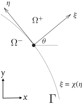
Figure 2.1: A diagram of the local coordinates in the normal and tangential directions, where θ is the angle between the x-axis and the normal direction.

(39)

use the local coordinates in the normal and tangential directions. Given a point (X, Y) on the interface, the local coordinate system in the normal and tangential directions is defined as (see Figure 2.1 for illustrations),

      

ξ = (x−X) cosθ+ (y−Y) sinθ η=−(x−X) sinθ+ (y−Y) cosθ

(2.11)

whereθis the angle between the x-axis and the normal direction ( ˆξ= ˆn), pointing to the Ω+ _{subdomain. Under such new coordinates system, the interface can be parameterized}

by

ξ =χ(η) with χ(0) = 0, χ0(0) = 0. (2.12)

where we assume that the interface is twice continuously differentiable, and henceχ0(0) = 0. The curvature of the interface at (X, Y) is χ00(0).

Consider the jumps across Γ at a fixed point (X, Y) that corresponds to the local coordinatesξ=η= 0. At this point, the solution ofProblem (II) will satisfy the following interface relations that represent the limiting values from one side of the interface in terms of the other using the local coordinates (2.11).

(40)

condi-tions (2.6a)–(2.6b)and the PDE (2.5a)–(2.5b), we have the following interface relations:

[u] =w,

[uξ] =g,

[uη] =w0,

[uηη] =−gχ00+w00, [uξη] =w0χ00+g0, [uξξ] =g

χ00− β

+

ξ

β+

−w00−

βξ

β

u−_ξ −

βη

β

u−_η − β

+

η

β+w

0 + f β , =g

χ00− β

− ξ

β−

−w00−

βξ

β

u+_ξ −

βη

β

u+_η − β

− η

β−w 0 + f β , (2.13)

where w0, g0 and w00 are the first- and second-order surface derivatives of w andg on the

interface, which are all evaluated at (ξ, η) = (0,0).

Proof:In a neighborhood of (X, Y), the interface can be expressed asξ =χ(η) with

χ(0) = 0 and χ0(0) = 0. Then the jump conditions w and g can be written as functions of only η. For simplicity, we still use the notation [u] =w(η) and [un] =g(η) in the local

coordinate system. Setting η = 0 in (2.6a) and (2.6b), we get the first two equalities in (2.13),

[u] =w(η) =⇒ [u] =w(0) =w, (2.14) [un] =g(η) =⇒ [uξ] =g(0) =g. (2.15) Differentiating the first jump condition ofProblem I in (2.6a) with respect toη along the interface, we get

[uξ]χ0 + [uη] =w0(η). (2.16)

(41)

again with respect toη, we obtain

[uξ]χ00+χ0

d

dη[uξ] + [uξη]χ

0

+ [uηη] =w00(η). (2.17)

Setting η= 0, we get the fourth equality in (2.13). Notice that in the local coordinates, the second jump condition of Problem II in (2.6b) can be written as

(u+_ξ −u+_ηχ0) = (u−_ξ −u−_ηχ0) +gp1 +χ02_. _(2.18)

Differentiating (2.18) with respect to η along the interface, we have

u+_ξξχ0+u+_ξη− d

dη(u +

η)χ 0₋

u+_ηχ00 = u_ξξ−χ0+u−_ξη − d

dη(u

− η)χ

0₋

u−_ηχ00

+g0(s)√1 +x02₊_g₍_s₎1

2

2χ0χ00

p

1 +χ02 .

(2.19)

Setting η = 0, we get the fifth equality in (2.13). Since the PDE in (2.5a)–(2.5b) are invariant under the transformation of the coordinates system in (2.11), we have

uξξ+uηη+

βξ

β uξ+ βη

β uη

= f β

=⇒ [uξξ] = −(−gχ00+w00)−

_β+

ξ

β+u +

ξ −

β_ξ− β−u

− ξ − _β+ η

β+u +

ξ −

β_η− β−u

− ξ − f β . (2.20)

Substituting u+_ξ =u−_ξ +g and u+

η =u − η +w

0 _{in the above equation, we get the first line} of the last equality in (2.13). Similarly, if we substitute u−_ξ =u+_ξ −g and u−_η =u+

η −w 0

in the above equation, we obtain the second line of the last equation in (2.13).

(42)

2.3

The augmented IIM

In Section 2.1, we introduced the jump in the normal derivative of the solution as the augmented variable and re-wrote the original interface problem as a Laplacian of the solution with lower order derivative terms. In Section 2.2, we derived jump relations for the solution, and its first order and second order derivatives in the local coordinates system. In this section, we use the IIM idea to discretize Problem (II) and derive the Schur complement system.

We first generate a uniform grid on the rectangular domain [a, b]×[c, d] where the elliptic interface problem is defined:

xi =a+ihx, yj =c+jhy, 0≤i≤N,0≤j ≤M (2.21)

where hx = (b−a)/N and hy = (d−c)/M. We assume that hx =hy =h for simplicity. We use the zero level set of a Liptschiz continuous function φ(x) defined on the entire domain (Ω+_∪_Ω−_∪_{Γ) to represent the interface. For example, if the interface is the unit} circle in two dimension, then the choice of a level set function isφ(x, y) =px2₊_y2₋_1.

The entire domain is then divided into two disjoint parts Ω− ={(x, y), φ(x, y)<0} and Ω+={(x, y), φ(x, y)>0} by the interface Γ ={(x, y), φ(x, y) = 0} .

To distinguish the discrete solution from the continuous solution, we use uppercase letters to indicate the solution of the discrete problem and lowercase letters for the continuous solutions. We also use bold letters for vectors.

(43)

anO(h2_{) local truncation error using the standard 5-point formula}

1

hx

β_i₊1 2,j

Ui+1,j−Ui,j

hx

−βi−1 2,j

Ui,j −Ui−1,j

hx

!

+ 1

hy

β_i,j₊1 2

Ui,j+1−Ui,j

hy

−β_i,j−1 2

Ui,j−Ui,j−1

hy

!

=fi,j,

=⇒ 1

βsum β_i₊1

2,j

Ui+1,j

h2 +βi−12,j

Ui−1,j

h2

+β_i,j₊1 2

Ui,j+1

h2 +βi,j−12

Ui,j−1 h2

!

− Ui,j

h2 = fi,j

βsum ,

(2.22)

where we have used the assumptionhx =hy =handβsum =βi+1/2,j+βi−1/2,j+βi,j+1/2+ βi,j−1/2. Since β(x, y) ≥ βmin > 0, the finite difference coefficients in (2.22) satisfy the

sign restrictions in (2.10).

We say (xi, yj) is an irregular grid point if the grid points in the standard five-point stencil centered at (i, j) are from both sides of the interface, as illustrated in Figure 2.2. We also wish to determine formula of the form (2.22) for the irregular points. Since these irregular points are adjacent to the interface Γ and form a lower dimensional set, it turns out to be sufficient to require anO(h) local truncation error at these points. To derive the finite difference scheme for the irregular points, we first write the PDE at the irregular point (xi, yj) as follows

uxx(xi, yj) +uyy(xi, yj) +

βx(xi, yj)

β(xi, yj)

ux(xi, yj) +

βy(xi, yj)

β(xi, yj)

uy(xi, yj) =

f(xi, yj)

β(xi, yj)

(2.23)

(44)

Figure 2.2: The geometry at an irregular grid point (xi, yj). The red diamonds are the control points, which are the orthogonal projections of the grid points (xi, yj+1) and

(xi+1, yj) on the interface. The blue triangles are the intersection points, where the in-terface intersects with the grid lines involved in the 5-point stencil.

and uy(xi, yj) are discussed in detail below.

2.3.1

Discretization of

u

xx

and

u

yy

at the irregular grid points

(45)

Figure 2.3: The irregular grid point (xi, yj) in the Ω− subdomain. At least one of its four nearest neighbor grid points must belong to the other subdomain Ω+_{. The intersections}

are labeled by the little blue triangles, with their coordinates listed inside the parentheses.

• When (i, j),(i−1, j)∈Ω−, while (i+ 1, j)∈Ω+ (see the left graph in Figure 2.3): Define an auxiliary function in the range x∈[xi−1, xi+1], y =yj

e

u(x) =

      

0 xi−1 ≤x≤x∗i+1,

[u]R+ [ux]R(x−x∗i+1) + [uxx]R

(x−x∗_i₊₁)2

2 x

∗

i+1 ≤x≤xi+1,

where x∗_i₊₁ is x-coordinate of the intersection point (Figure 2.3) and [u]R, [ux]R and [uxx]R are the jumps at the intersection point (x∗i+1, yj) on the right hand side of (i, j). Then, we define another function q(x) = u(x, yj)−ue(x), which satisfies

(46)

Figure 2.4: The irregular grid point (xi, yj) in Ω+ subdomain. At least one of its four nearest neighbor grid points must belong to the other subdomain Ω−. The intersections are labeled by the little blue triangles, with their coordinates listed inside the parentheses.

u(x, yj) =q(x) in the neighborhood of xi, we have

uxx(xi, yj) = qxx(xi) =

Qi+1−2Qi+Qi−1 h2

x

+O(h2_x) = Ui+1,j−2Ui,j+Ui−1,j

h2

x

−

[u]R+ [ux]RdR+ [uxx]R

d2_R

2

h2

x

+O(h2_x),

(2.24)

where dR=xi+1−x∗i+1.

• When (i, j),(i+ 1, j)∈Ω−, while (i−1, j)∈Ω+ _{(see the right graph in Figure 2.3):}

Define an auxiliary function in the range x∈[xi−1, xi+1], y =yj

e

u(x) =

      

[u]L+ [ux]L(x−x∗i−1) + [uxx]L

(x−x∗_i−₁)2

2 xi−1 ≤x≤x ∗ i−1,

0 x∗_i−₁ ≤x≤xi+1,

(47)

[uxx]Lare the jump relations at the intersection point (x∗i−1, yj) on the left hand side of (i, j). Then, we define another function q(x) = u(x, yj)−ue(x), which satisfies

[q] = [qx] = [qxx] = 0. That says q(x) is twice continuously differentiable. Since

u(x, yj) =q(x) in the neighborhood of xi, we have

uxx(xi, yj) =qxx(xi) =

x

+O(h2_x) = Ui+1,j−2Ui,j +Ui−1,j

h2

x

−

[u]L+ [ux]LdL+ [uxx]L

d2

L 2

h2

x

+O(h2_x),

(2.25)

where dL=xi−1−x∗i−1.

• When (i, j)∈Ω−, while (i−1, j),(i+ 1, j)∈Ω+:

Define an auxiliary function in the range x∈[xi−1, xi+1], y =yj

e

u(x) =

              

[u]L+ [ux]L(x−x∗i−1) + [uxx]L

(x−x∗_i−₁)2

2 xi−1 ≤x≤x ∗ i−1,

0 x∗_i−₁ ≤x≤x∗_i₊₁,

[u]R+ [ux]R(x−x∗i+1) + [uxx]R

(x−x∗_i₊₁)2

2 x

∗

i+1 ≤x≤xi+1,

where x∗_i−₁ and x∗_i₊₁ are x-coordinates of the intersection points (Figure 2.3) and [u]L/R, [ux]L/Rand [uxx]L/Rare the jumps at the intersection point (x∗i−1, yj)/(x∗i+1, yj) on the left/right hand side of (i, j). Then, we define another function q(x) =

u(x, yj)− eu(x), which satisfies [q] = [qx] = [qxx] = 0. That says q(x) is twice

(48)

have

uxx(xi, yj) = qxx(xi) =

x

+O(h2_x) = Ui+1,j−2Ui,j+Ui−1,j

h2

x

−

d2_L

2

h2

x

−

d2_R

2

h2

x

+O(h2_x),

(2.26)

where dL=xi−1−x∗i−1 and dR =xi+1−x∗i+1.

Similarly, to discretize uyy(xi, yj), we need the two nearest neighbor points from the up side (i, j+ 1) and the down side (i, j−1). Their positions with respect to the interface could also have three possibilities as listed below.

• When (i, j),(i, j−1)∈Ω−, while (i, j+ 1)∈Ω+ _{(see the left graph in Figure 2.3):}

Define an auxiliary function in the range y∈[yj−1, yj+1], x=xi

e

u(y) =

      

0 yj−1 ≤x≤yj∗+1,

[u]U+ [uy]U(y−y_j∗₊₁) + [uyy]U(y−y ∗ j+1)2

2 y

∗

j+1 ≤y≤yj+1, where y_j∗₊₁ is y-coordinate of the intersection point (Figure 2.3) and [u]U, [uy]U and [uyy]U are the jump relations at the intersection point (xi, yj∗+1) on the up side

of (i, j). Then, we define another function q(y) = u(xi, y)−eu(y), which satisfies

(49)

u(xi, y) =q(y) in the neighborhood ofyj, we have

uyy(xi, yj) =qyy(yj) =

Qj+1−2Qj+Qj−1 h2

y

+O(h2_y) = Ui,j+1−2Ui,j +Ui,j−1

h2

y

−

[u]U+ [uy]UdU + [uyy]U

d2

U 2

h2

y

+O(h2_y),

(2.27)

where dU =yj+1−y∗j+1.

• When (i, j),(i, j+ 1)∈Ω−, while (i, j−1)∈Ω+ _{(see the right graph in Figure 2.3):}

e

u(y) =

      

[u]D+ [uy]D(y−yj−∗ 1) + [uyy]D

(y−y_j−∗ ₁)2

2 yj−1 ≤y ≤y ∗ j−1,

0 y∗_j−₁ ≤y ≤yj+1,

wherey_j−∗ ₁ isy-coordinate of the intersection point (Figure 2.3) and [u]D, [uy]D and [uyy]D are the jump relations at the intersection point (xi, y∗j−1) on the down side

of (i, j). Then, we define another function q(y) = u(xi, y)−eu(y), which satisfies

[q] = [qy] = [qyy] = 0. That says q(y) is twice continuously differentiable. Since

u(xi, y) =q(y) in the neighborhood ofyj, we have

uyy(xi, yj) = qyy(yj) =

Qj+1−2Qj +Qj−1 h2

y

+O(h2_y) = Ui,j+1−2Ui,j +Ui,j−1

h2

y

−

[u]D+ [uy]DdD+ [uyy]D

d2

D 2

h2

y

+O(h2_y),

(50)

where dD =yj−1−y∗j−1.

• When (i, j)∈Ω−, while (i, j−1),(i, j+ 1)∈Ω+_:

e

u(y) =

              

[u]D+ [uy]D(y−yj−∗ 1) + [uyy]D

(y−y_j−∗ ₁)2

2 yj−1 ≤y ≤y ∗ j−1,

0 y∗_j−₁ ≤y ≤y_j∗₊₁,

[u]U+ [uy]U(y−yj∗+1) + [uyy]U

(y−y_j∗₊₁)2

2 y

∗

j+1 ≤y ≤yj+1,

where yj−∗ 1 and yj∗+1 are y-coordinates of the intersection points (Figure 2.3) and

[u]D/U, [uy]D/U and [uyy]D/U are the jumps at the intersection point (xi, yj−∗ 1)/(xi, y∗j+1)

on the down/up side of (i, j). Then, we define another function q(y) = u(xi, y)−

e

u(y), which satisfies [q] = [qy] = [qyy] = 0. That says q(y) is twice continuously differentiable. Since u(xi, y) =q(y) in the neighborhood ofyj, we have

uyy(xi, yj) =qyy(yj) =

Qj+1−2Qj+Qj−1 h2

y

+O(h2_y) = Ui,j+1−2Ui,j +Ui,j−1

h2

y

−

d2_D

2

h2

y

−

[u]U+ [uy]UdU + [uyy]U

d2

U 2

h2

y

+O(h2_y),

(2.29)

where dD =yj−1−y∗j−1 and dU =yj+1−y∗j+1.

So far, we have obtained the discretization scheme for the differential operators

(51)

(xi, yj) lies in the Ω+ domain, we can follow exactly the same procedures above to de-rive the corresponding discrete forms. Here, for the case when the irregular grid point (i, j)∈Ω+ _{(see Figure 2.4), the only difference we need to make is to define} _q ₌_u₊

e

u , instead of q =u−_eu as used in the above analysis for (i, j)∈Ω−. This thus will change the “−” before the correction terms in (2.24)–(2.29) to the “+” sign in the discrete forms. We summarize the results in the following two equations. The discretization ofuxx(xi, yj) for (i, j)∈Ω+ is

uxx(xi, yj) =

                                     ∇2

hx +

d2_R

2

h2

x

+O(h2

x) only (i+ 1, j)∈Ω −_,

∇2

hx +

d2

L 2

h2

x

+O(h2

x) only (i−1, j)∈Ω −_,

∇2_h_x +

d2 R 2 h2 x +

d2

L 2

h2

x

+O(h2_x)

both (i±1, j)∈Ω−,

(2.30) where ∇2

hx =

Ui+1,j−2Ui,j+Ui−1,j

h2

x

(52)

defined in (2.24)–(2.26). The discretization of uyy(xi, yj) for (i, j)∈Ω+ is

uyy(xi, yj) =

                                       ∇2

hy+

[u]U + [uy]UdU + [uyy]U

d2

U 2

h2

y

+O(h2

y) only (i, j+ 1)∈Ω −_,

∇2

hy+

[u]D + [uy]DdD + [uyy]D

d2_D

2

h2

y

+O(h2

y) only (i, j−1)∈Ω −_,

∇2_h_y+

[u]U + [uy]UdU + [uyy]U

d2 U 2 h2 y +

d2

D 2

h2

y

+O(h2_y)

both (i, j ±1)∈Ω−,

(2.31) where ∇2

hy =

Ui,j+1−2Ui,j +Ui,j−1 h2

y

and [u]U/D, [ux]U/D, [uxx]U/D, dU/D are previously defined in (2.27)–(2.29).

2.3.2

Jumps at the intersections

(53)

operators in the local coordinate system and Cartesian coordinate system, which satisfies    ∂ ∂x ∂ ∂y   =   

cosθ −sinθ

sinθ cosθ

      ∂ ∂ξ ∂ ∂η    ,    ∂ ∂ξ ∂ ∂η   =   

cosθ sinθ

−sinθ cosθ

      ∂ ∂x ∂ ∂y    ,    ∂2 ∂x2 ∂2 ∂y2   =   

cos2θ −2 sinθcosθ sin2θ

sin2θ 2 sinθcosθ cos2θ

         ∂2 ∂ξ2 ∂2 ∂ξ∂η ∂2 ∂η2       , (2.32)

where the differential operators could act on any functions, for example, the solution

u(x, y).

(54)

operator relations in (2.32), we have

[u] =w,

[ux] = cosθ[uξ]−sinθ[uη] =gcosθ−w0sinθ ,

[uy] = sinθ[uξ] + cosθ[uη] =gsinθ+w0cosθ , [uxx] = cos2θ[uξξ]−2 sinθcosθ[uξη] + sin2θ[uηη]

=−2 sinθcosθ(w0χ00+g0) + sin2θ(−gχ00+w00) + cos2θn g(χ00−β

+

ξ

β+)−w

00₋ β

+

η

β+w

0 + f β − βξ β

(cosθu−_x + sinθu−_y)−

βη

β

(−sinθu−_x + cosθu−_y)o,

[uyy] = sin2θ[uξξ] + 2 sinθcosθ[uξη] + cos2θ[uηη] = 2 sinθcosθ(w0χ00+g0) + cos2θ(−gχ00+w00)

+ sin2θn g(χ00−β

+

ξ

β+)−w

00₋ β

+

η

β+w

0₊ f β − βξ β

(cosθu−_x + sinθu−_y)−

βη

β

(−sinθu−_x + cosθu−_y)

o

,

(2.33)

where u−_x and u−_y can be further approximated by ux(xi, yj) and uy(xi, yj) at the center grid point (i, j) using Taylor expansion. That says, since the distance between the inter-section point and the center point (i, j) is less than or equal to hx orhy (see Figure 2.3), we can write

u−_x|intersection=ux(xi, yj) +O(hx),

u−_y|intersection=uy(xi, yj) +O(hy).

(2.34)

Similarly, in the case (i, j) ∈ Ω+_{, we need to choose the alternative formula for the}

(55)

become

[uxx] = cos2θ[uξξ]−2 sinθcosθ[uξη] + sin2θ[uηη] =−2 sinθcosθ(w0χ00+g0) + sin2θ(−gχ00+w00)

+ cos2θn g(χ00− β

− ξ

β−)−w 00₋ β

− η

β−w 0 + f β − βξ β

(cosθu+_x + sinθu+_y)−

βη

β

(−sinθu+_x + cosθu+_y)o,

[uyy] = sin2θ[uξξ] + 2 sinθcosθ[uξη] + cos2θ[uηη] = 2 sinθcosθ(w0χ00+g0) + cos2θ(−gχ00+w00)

+ sin2θn g(χ00−β

− ξ

β−)−w 00₋ β

− η

β−w 0 + f β − βξ β

(cosθu+_x + sinθu+_y)−

βη

β

(−sinθu+_x + cosθu+_y)o,

(2.35)

where u+

x and u+y can be further approximated by ux(xi, yj) and uy(xi, yj) at the center grid point (i, j) using Taylor expansion. Since the distance between the intersection point and the center point (i, j) is less than or equal to hx orhy (see Figure 2.4), we can write

u+_x|intersection=ux(xi, yj) +O(hx),

u+_y|intersection=uy(xi, yj) +O(hy).

(2.36)

Substituting (2.33) and (2.35) to the discrete forms of uxx and uyy in (2.24)–(2.29), and collecting terms ux(xi, yj) and uy(xi, yj), we have

uxx(xi, yj) +uyy(xi, yj) =∇2hu(xi, yj) +k1ux(xi, yj) +k2uy(xi, yj) +C1+O(max{hx, hy}),

(56)

where ∇2

hu(xi, yj) =

Ui+1,j+Ui−1,j−2Ui,j

h2

x

+ Ui,j+1+Ui,j−1 −2Ui,j

h2

y

and k1, k2, C1 are

constant correction terms. Notice that k1 and k2 are independent of the jump conditions g,wand their surface derivativesg0,w0 andw00 at the intersections ( see (2.33) and (2.35) for details), while the constant C1 is a function of g, w and their surface derivatives at the intersection points. Therefore, the PDE at the irregular grid point (xi, yj) in (2.23) becomes

∇2

hu(xi, yj) +

β_x(x_i, y_j)

β(xi, yj) +k1

ux(xi, yj) +βy(xi, yj)

β(xi, yj) +k2

uy(xi, yj) =

f(xi, yj)

β(xi, yj)

−C1+O(max{hx, hy}) ,

(2.38)

where∇2

hu(xi, yj) =

Ui+1,j +Ui−1,j−2Ui,j

h2

x

+Ui,j+1+Ui,j−1−2Ui,j

h2

y

is the discrete Lapla-cian operator. We still need to derive the discrete forms for ux(xi, yj) and uy(xi, yj).

2.3.3

Discretization of

u

x

and

u

y

at the irregular grid points

We use the two point stencil for the first order derivatives ux(xi, yj) and uy(xi, yj). We first consider the discretization of ux(xi, yj). If the coefficient (β_βx +k1) before ux(xi, yj) in (2.38) is positive , we use (i, j) and the grid point on the right (i+ 1, j) to approximate

ux(xi, yj). Otherwise, we use (i, j) and the grid point on the left (i−1, j) to approximate

ux(xi, yj). The stencil points are chosen in this way to satisfy the sign restrictions of the finite difference coefficients in (2.10). So, we have

ux(xi, yj) =

      

Ui+1,j−Ui,j

hx +CR+O(hx) if (

βx

β +k1)>0, Ui,j−Ui−1,j

hx +CL+O(hx) if (

βx

β +k1)≤0,

(57)

where both CR and CL are constants that are determined by the positions of the two point stencil relative to the interface Γ . CR = 0 when (i, j) and (i+ 1, j) are from the same side of the interface. Similar, CL = 0 if (i, j) and (i−1, j) are from the same side of the interface.

However, when the two grid points of the stencil are on different sides of the interface, we need to derive the nonzero constants CR and CL.

For CR, the two grid points involved are (i, j) and (i+ 1, j), and their positions with respect to the interface could have two possibilities as listed below.

• When (i, j)∈Ω−, while (i+ 1, j)∈Ω+ _{( see the left graph in Figure 2.3): We define}

an auxiliary function in the range x∈[xi−1, xi+1], y =yj

e

u(x) =

      

0 xi−1 ≤x≤x∗i+1,

[u]R+ [ux]R(x−x∗_i₊₁) x∗_i₊₁ ≤x≤xi+1,

(2.40)

wherex∗_i₊₁ isx-coordinate of the intersection point (Figure 2.3) and [u]Rand [ux]R are the jumps at the intersection point (x∗_i₊₁, yj) on the right hand side of (i, j). Then, we define another function q(x) = u(x, yj) − eu(x), which satisfies [q] =

[qx] = 0. That says q(x) is continuously differentiable. Sinceu(x, yj) = q(x) in the neighborhood of xi, we have

ux(xi, yj) =qx(xi) =

Qi+1−Qi

hx

+O(hx) = Ui+1,j−Ui,j

hx

− [u]R+ [ux]RdR

hx

+O(hx) =⇒CR=−

[u]R+ [ux]RdR

hx

(2.41)

(58)

• When (i, j) ∈ Ω+_{, while (}_i_{+ 1}_{, j}₎ _∈ _Ω− _{( see the left graph in Figure 2.4): We} define the same auxiliary functionu_e(x) in (2.40). Then, we define another function

q(x) = u(x, yj) +ue(x). Notice here we use “+” instead of “−” sign betweenu(x, yj)

and _eu(x) since (i, j) is in the Ω+ _{domain now. The} _q₍_x_{) function satisfies [}_q_{] =}

[qx] = 0. That says q(x) is continuously differentiable. Sinceu(x, yj) = q(x) in the neighborhood of xi, we have

Qi+1−Qi

hx

+O(hx) = Ui+1,j−Ui,j

hx

+[u]R+ [ux]RdR

hx

+O(hx) =⇒CR=

[u]R+ [ux]RdR

hx

(2.42)

where dR=xi+1−x∗i+1.

For CL, the two grid points involved are (i, j) and (i−1, j), and their positions with respect to the interface could also have two possibilities as listed below.

• When (i, j) ∈ Ω−, while (i−1, j) ∈ Ω+ ( see the right graph in Figure 2.3): We define an auxiliary function in the rangex∈[xi−1, xi+1], y =yj

e

u(x) =

      

[u]L+ [ux]L(x−xi−∗ 1) xi−1 ≤x≤x∗i−1,

0 x∗_i−₁ ≤x≤xi+1,

(2.43)

wherex∗_i−₁ isx-coordinate of the intersection point (Figure 2.3) and [u]L and [ux]L are the jump relations at the intersection point (x∗_i−₁, yj) on the left hand side of (i, j). Then, we define another function q(x) = u(x, yj)−ue(x), which satisfies

(59)

in the neighborhood of xi, we have

Qi−Qi−1 hx

+O(hx) = Ui,j −Ui−1,j

hx

− [u]L+ [ux]LdL

hx

+O(hx) =⇒CL =−

[u]L+ [ux]LdL

hx

(2.44)

where dL=xi−1−x∗i−1.

• When (i, j) ∈ Ω+, while (i− 1, j) ∈ Ω− ( see the right graph in Figure 2.4): We define the same auxiliary function u_e(x) in (2.43). Then, we define another functionq(x) =u(x, yj)+ue(x). Notice here we use “+” instead of “−” sign between

u(x, yj) and eu(x) since (i, j) is in the Ω

+ _{domain now. The} _q