Adaptability and Comparison of the Wavelet-based with Traditional Equivalent Linearization Method and Potential Application for Damage Detection

Abstract

CAO, YINGFANG. Adaptability and Comparison of the Wavelet-based with Traditional

Equivalent Linearization Method and Potential Application for Damage Detection.

(Under the direction of Mohammad N. Noori.)

The main objective of this research work is to compare a wavelet transform based

Equivalent linearization technique, presented herein with the traditional Equivalent

linearization method. In addition, the application of this wavelet-base method to the

damage detection of a single Degree of Freedom system has also been presented.

In many practical applications the system of concern is nonlinear. In general, and

especially in random vibration analysis, it is difficult to obtain a closed form solution for

dynamic response of a nonlinear system. Therefore, it is necessary to replace the

nonlinear system with an equivalent linear system. Method of equivalent linearization has

been extensively used in these engineering applications. The wavelet analysis allows us

to capture temporal variations in the energy and frequency content. In combining the

wavelet analysis technique and the well-known Equivalent linearization method, a

nonlinear system can be approximated as a time dependent linear system. By comparing

the information of the time-varying natural frequency coefficient between the healthy

system and the damaged system, the introduced damage can be identified at a particular

time.

The first part of this document consists of a detailed description of some of the most

common types of time-frequency methods that have been developed or used for vibration

Equivalent Linearization Method have been introduced to demonstrate the general

procedure to linearize a system. An important linearization method, utilizing Wavelet

based transformation is then presented.

In this study, the benefits of this proposed method have been verified by its

application in a typical nonlinear system. Different wavelets and different excitations are

used in performing this analysis. To verify the accuracy of the wavelet based method, the

traditional Equivalent Linearization results of displacement have been compared with

those obtained by this method. In order to check the feasibility of the methodology, the

relationship of the restoring force vs. displacement has been compared between the

original nonlinear system and the equivalent linear system. For further application in the

structural health monitoring, this method has been applied to some simple cases to see the

effect of damage detection. To simplify the entire procedure of derivation, some

formulation work introduced by Basu, Gupta [1997] and Roberts and Spanos [1990] have

been followed.

ADAPTABILITY AND COMPARISON OF THE WAVELET-BASED WITH TRADITIONAL EQUIVALENT LINEARIZATION METHOD AND POTENTIAL

APPLICATION FOR DAMAGE DETECTION

by Yingfang Cao

A thesis submitted to the Graduate Faculty of North Carolina State University

in partial fulfillment of the requirements for the Degree of

Master of Science

MECHANICAL ENGINEERING

Raleigh

Biography

The author of this thesis was born in Shanxi Province, P.R. China on September

1975. Graduating from high school from the first high school in Xinzhou, P. R. China on

1993, she began her college education at the University of Science and Technology in

Beijing, and graduated in 1997 with a Bachelor in Science in Mechanical Engineering. In

2001, she began her graduate studies at North Carolina State University under the

Acknowledgements

Certainly, the completion of this work would have not been possible without having

God’s help all along the way. Also, this work would have not been possible without the

help and support of my parents. Special thanks to them for showing me, among all things,

the values of hard work and perseverance. Thanks also to my husband, Weijun Guo,

thanks for your constant support, and for providing me enthusiasm when it was most

needed. Also thanks to the rest of the members of my family for their endless support

throughout this time.

To Dr. Mohammad N. Noori my sincere thanks for allowing me to work with him for

this past years. Thanks for your trust, guidance and advices important for the completion

of this work. Special thanks to Dr. Hou and Dr. Arata Masuda for their continuous and

invaluable help and comments, and with whom it was a pleasure to work with. I will also

like to mention and thank the faculty at the Mechanical and Aerospace Engineering

Department and the Electrical Engineering Department at North Carolina State,

especially Dr. Yuan and Dr. Krim, for being part of my committees.

In addition thanks to all the friends, especially to those who have being around me

Table of Contents

LIST OF FIGURES... VI

CHAPTER 1 : INTRODUCTION ...1

1.1 TIME-FREQUENCY ANALYSIS...1

1.2 EQUIVALENT LINEARIZATION METHOD...4

1.3 STRUCTURAL HEALTH MONITORING...6

1.4 SCOPES...10

CHAPTER 2 : FOURIER ANALYSIS...13

2.1 FOURIER SERIES...13

2.2 FOURIER TRANSFORM...15

2.2.1 Definition...15

2.2.2 Properties of the Fourier Transform ...16

2.3 DISCRETE FOURIER TRANSFORM...18

2.4 FAST FOURIER TRANSFORM...19

2.5 APPLICATION OF THE FOURIER TRANSFORM...20

2.6 SUMMARY...21

CHAPTER 3 : INTRODUCTION OF TIME-FREQUENCY ANALYSIS...22

3.1 INTRODUCTION...22

3.2 UNCERTAINTY PRINCIPLES...22

3.3 SHORT TIME FOURIER TRANSFORM (STFT)...25

3.3.1 Definition...25

3.3.2 Remarks...27

3.3.3 Disadvantages ...27

3.4 WIGNER-VILLE DISTRIBUTION (WVD) ...28

3.4.1 Definition...28

3.4.2 Properties ...30

3.4.3 Disadvantages ...31

CHAPTER 4 : WAVELET TRANSFORM (WT) ...32

4.1 WHAT ARE WAVELETS...32

4.2 CONTINUOUS WAVELET TRANSFORM (CWT)...35

4.2.1 Definition...36

4.2.2 Properties of CWT ...40

4.2.3 Computation of CWT ...47

4.3 DISCRETE WAVELET TRANSFORM (DWT)...50

4.3.1 Definition...50

4.3.2 Multiresolution Analysis ...54

4.3.3 Wavelet Reconstruction...58

CHAPTER 5 : GENERAL EQUIVALENT LINEARIZATION METHOD...61

5.1 INTRODUCTION...61

5.1.2 Markov method ...62

5.1.3 Monte Carlo Simulation...62

5.1.4 Stochastic Equivalent Linearization ...63

5.2 STOCHASTIC EQUIVALENT LINEARIZATION METHOD...63

5.2.1 System model ...64

5.2.2 Implementation of the Stochastic Equivalent Linearization...65

CHAPTER 6 : WAVELET-BASED STOCHASTIC LINEARIZATION ...69

6.1 INTRODUCTION...69

6.2 INPUT-OUTPUT RELATIONSHIP FOR A LINEAR SYSTEM...70

6.2.1 Review of Wavelet Theory ...70

6.2.2 Input-output relation...71

6.3 WAVELET-BASED EQUIVALENT LINEARIZATION...73

6.4 IMPLEMENTATION TO DUFFING OSCILLATOR...74

CHAPTER 7 : NUMERICAL SOLUTIONS ...77

7.1 COMPARISON OF THE WAVELET-BASED AND TRADITIONAL EQL ...77

7.2 EFFECTS OF THE NONLINEARITY...81

7.3 DAMAGE DETECTION...85

CHAPTER 8 : CONCLUSIONS AND RECOMMENDATIONS ...89

8.1 CONCLUSIONS...89

8.1.1 Wavelet-based Equivalent Linearization Method...89

8.1.2 Nonlinearity effects ...90

8.1.3 Damage Detection ...91

8.2 RECOMMENDATIONS...91

List of Figures

FIGURE 4.1 COMPARISON OF THE SINE WAVE...33

FIGURE 4.2 DAUBECHIES WAVELETS...34

FIGURE 4.3 MORLET AND MEXICAN HAT WAVELET FORMS...35

FIGURE 4.4 SCALING AND SHIFTING OF A WAVELET...38

FIGURE 4.5 SCALE EFFECT ON FREQUENCY DOMAIN...39

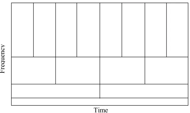
FIGURE 4.6 TIME AND FREQUENCY RESOLUTION OF THE WAVELET TRANSFORM...41

FIGURE 4.7 PROCESS OF THE WAVELET TRANSFORM...47

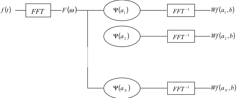
FIGURE 4.8 SCHEMATIC OF THE FREQUENCY-BASED ALGORITHM OF CWT ...49

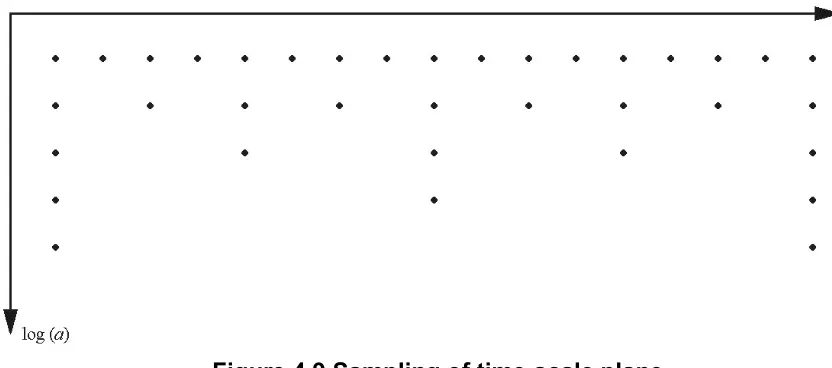
FIGURE 4.9 SAMPLING OF TIME-SCALE PLANE...52

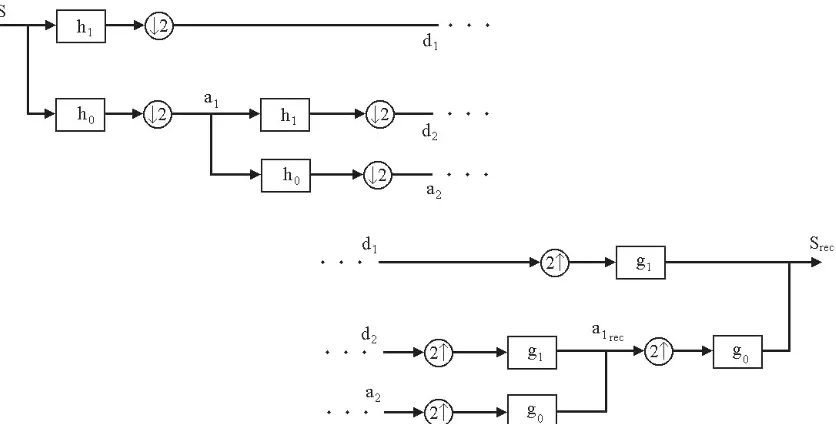
FIGURE 4.10 TREE ALGORITHMS FOR WAVELET DECOMPOSITION AND RECONSTRUCTION...60

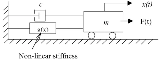
FIGURE 5.1 SDOF MASS-SPRING-DAMPER SYSTEM...64

FIGURE 7.1 EXCITATION 1- EL CENTRO EARTHQUAKE ACCELERATION...78

FIGURE 7.2USING MEXICAN HAT WAVELET...79

FIGURE 7.3USING MORLET WAVELET...79

FIGURE 7.4EXCITATION 2-WHITE NOISE...80

FIGURE 7.5 COMPARISON OF DIFFERENT METHOD UNDER WHITE NOISE EXCITATION...81

FIGURE 7.6 RESTORING FORCE VS. DISPLACEMENT WITH SMALL NONLINEARITY...82

FIGURE 7.7 RESPONSE RESULTS WITH NONLINEAR FACTOR λ=3 ...83

FIGURE 7.8RESTORING FORCE VS. DISPLACEMENT FOR CASE FOR λ=3 ...84

FIGURE 7.9 RESTORING FORCE VS. DISPLACEMENT FOR CASE FOR λ=5...84

FIGURE 7.10 RESTORING FORCE VS. DISPLACEMENT FOR CASE FOR λ=5...85

FIGURE 7.11 DISPLACEMENT RESPONSE OF THE DAMAGED SYSTEM...86

FIGURE 7.12 EQUIVALENT TIME-VARYING NATURAL FREQUENCY OF THE HEALTH SYSTEM...87

Chapter 1 : Introduction

1.1 Time-Frequency Analysis

Time-frequency analysis plays a central role in signal analysis. Time-frequency

methods are simply the extensions of the well-known Fourier Transform (FT) in which

most signals of practical interest can be decomposed into a sum of sinusoidal components

with different frequencies. As a tool for applications, Fourier Transform is used in

virtually all areas of science and engineering, especially in its discrete form since

computational power has increased dramatically. Fourier Transform demonstrates that

every signal has a spectrum, while the Fourier inversion theorem implies that a function

and its Fourier transform are really equivalent in the sense that one determines the other.

The invention of the computer algorithm known as the Fast Fourier Transform (FFT) in

the mid-1960s opened up the possibility of an even wider use of the FT in computational

physics and many other areas of Physics and Mathematics. Nowadays, computers being

used in computational physics are frequently evaluated principally on their capacity to

perform the FFT algorithm, and many special computers or add-on cards are available to

perform the FFT algorithm at ultra-high speed.

Even after the introduction of the FFT algorithm, the Fourier Transform still faces

some limitations. In many applications, the system being studied generates quickly

changing (impulsive) sounds or vibrations. The Fourier Transform cannot provide

temporal localization necessary for proper engineering analysis. This characteristic makes

it only suitable for the analysis of stationary signals where the frequency content of the

a new tool, which can be used to give information about signals simultaneously in the

time domain and the frequency domain.

One of the first time-frequency representations developed is the Wigner-Ville

transform. In 1932, Wigner derived a distribution over the phase space in quantum

mechanics [Wigner, 1932]. Some 15 years later, Ville, searching for an ``instantaneous

spectrum'' - influenced by the work of Gabor - introduced the same transform in signal

analysis [Ville, 1948]. Unfortunately the non-linearity of the Wigner distribution causes

many interference phenomena, which makes it less attractive for many practical purposes

[Cohen, 1995].

A different approach to obtain a local time-frequency analysis (suggested by various

scientists, among them Ville), is to cut the signal first into slices, followed by doing a

Fourier analysis on these slices. But the functions obtained by this crude segmentation are

not periodic, which will be reflected in large Fourier coefficients at high frequencies,

since the Fourier transform will interpret this jump at the boundaries as a discontinuity or

an abrupt variation of the signal. To avoid these artifacts, the concept of windowing has

been introduced. By segmenting the signal into small sections and analyzing each section

separately there is a better chance to procure meaningful analysis. If the signal has sharp

transitions, windowing the input data such that the sections converge to zero at the

endpoints helps to localize the signal in time. Adjacent sequences of windowed Fourier

analyses join together to produce a time ordered view of the frequency content of a

signal.

While the windowed Fourier Transform compromise between the time and frequency

window is chosen, that window is same for all frequencies. Many signals require a more

flexible approach—varying the window size to determine more accurately either time or

frequency.

A revolutionary change from the concept of time-frequency analysis came with the

introduction of Wavelet Transform (WT). Wavelet theory was initially proposed by J.

Morlet, a geophysicist, and A. Crossman, a theoretical physicist [1984], together with

their fellow Frenchman, Y. Meyer, their ‘French school’ developed the mathematical

foundations of wavelets. Due to its mathematical complexity, the wavelet analysis

remained purely theoretical and had very limited practical applications at that time. It was

the work of Daubechies [1988,1990,1992], and Mallat [1989], which established the

necessary links between the rigorous mathematical requirements and the wide

applications in signal processing.

Wavelet analysis allows the use of long time intervals where more precise

low-frequency information can be obtained and shorter regions where high-low-frequency

information can be gained. Instead of breaking down the signal into harmonics, the

Wavelet Transform break down the signal into a series of local basis functions called

wavelets. These basis functions are nothing but variable length window functions, where

the length depends on a variable scale parameter. This scale parameter then could be

related to a center frequency of the window and thus allowing for the construction of a

time-frequency map of the signal. Compared with sine waves, wavelets tend to be

irregular and asymmetric. Signals with sharp changes might be better analyzed with an

irregular wavelet than with a smooth sinusoid. With its capability of revealing the aspects

great acceptance in several fields, especially in the applications of image processing

which take great advantage of the variable window property of this new transform. This

same property will be the one, which will pose the Wavelet transform as a useful tool for

structural health monitoring applications.

1.2 Equivalent Linearization Method

In many practical applications, due to the high intensity nature and often complex

nature of environmental loads such as earthquakes, wind loads, and sea waves, the

systems subjected to these loadings may experience excessive stress or displacements

that results in elastic or even hysteretic behavior. This is particularly the case under high

intensity random excitation. Under these conditions, it is difficult to obtain the closed

form solution for dynamic response of a nonlinear system. Therefore, for higher

accuracy, one must resort to the analysis of nonlinear systems under non-stationary

forces.

Of the various possible approaches that are available, over last several decades, the

method of equivalent linearization has been proved to be the most useful approximation

technique and has been extensively used in engineering applications. Basically, the

method is the statistical extension of Krylov and Bogoliubov’s [1963] linearization

technique and is often referred to as the ‘describing function method’ in the electrical

engineering literature. An adaptation of the approach to deal with stochastic problems

was originally developed by Booton [1953] and used as a tool in control engineering.

Subsequent developments of this method in this field have been described by Sawaragi

[1962], Kazakov [1965], Gelb and Van Der Velde [1968], Atherton [1975] and Sinitsyn

Independently, the method, (now variously known as ‘statistical linearization’ or

‘equivalent linearization’) was proposed by Caughey [1963] as a means of solving

nonlinear stochastic problems in structural dynamics. With Caughey’s work, the linear

part of the nonlinear equation was uncoupled using the modal matrix, and then

linearization technique was applied to the resulting single-degree-of-freedom equations

separately. This is quite effective when applicable, but the conditions imposed on the

instantaneous correlation matrix of the excitation limited its application except for some

special cases. In Foster’s (1968) more general approach, numerical methods must be used

in order to obtain the equivalent linear stiffness and damping matrices. By this way, the

procedure of approximating closed form solutions would require an excessive amount of

algebraic computation. Later on, Iwan and Yang (1971 and 1972) were able to formulate

the approach such that the linear stiffness and damping matrices may be determined

analytically. Their approach is based on the concept of decomposing the nonlinear forces

of the actual system into the sum of simpler approximate nonlinear forces, each of which

depends solely on the relative displacement and velocity between discrete masses of the

system. In some cases, this method will yield closed form solutions. However, given a

system of nonlinear equations, accuracy of the solution depends heavily on the choice of

these approximate forces. Also, when the masses are distributed, the identification of the

forces might be quite complex.

This approach is well suited to mass-spring type systems. Numerous applications of

the technique for studying the response of non-linear oscillators to random excitation

have been described in the literatures [Roberts, 1981b, and Spanos, 1981a]. Although

has proved a useful analytical tool across a very wide spread of engineering applications

[Roberts and Spanos, 1990], generally, in this technique, the excitations are assumed to

be stationary and gaussian. Thus, in some cases, such as systems excited by ground

motion, it is necessary to approximate the nonlinear system to be a time-varying system.

Some theoretical developments in this area have been illustrated by Spanos [1978,1980

and 1981], Iwan and Mason [1980], Ahmadi [1980], and Noori et. al. [1986].

In recent years, it has been shown that Wavelet analysis provides a convenient way

for the response analysis of systems subjected to non-stationary ground motion (Basu,

Gupta, [1997]). Specifically, the wavelet transformation has been used to obtain both

frequency and temporal information of system response caused by non-stationary

excitation. Based on this capability, the wavelet analysis method can be combined with

traditional equivalent linearization method to obtain a time-varying equivalent system

[Basu and Gupta, 1999]. This recently developed wavelet-based equivalent linearization

method has proved to be more accurate when dealing with some nonlinear SDOF

structures [Cao and Noori, 2002].

1.3 Structural Health Monitoring

Nearly all in-service structures require some form of maintenance for monitoring

their integrity and health condition to prolong their lifespan or to prevent catastrophic

failure. The interest in the ability to monitor a structure and detect damage at the earliest

possible stage is pervasive throughout the civil, mechanical and aerospace engineering

communities. This is now commonly referred to as ‘Structural Health Monitoring and

Structural health monitoring can be defined as the diagnostic monitoring of the

integrity or condition of a structure. The intent is to detect and locate damage or

degradation in structural components and to provide this information quickly and in a

form easily understood by the operators or occupants of the structure. The damage may

result from fatigue, large earthquake, strong winds, and explosion or vehicle impact.

Early detection of damage or structural degradation prior to local failure can prevent

"runaway" catastrophic failure of the system. In engineering applications, damage is

understood intuitively as an imperfection or impairment of the function and working

condition of a structure or machine. Damage can be described in many ways depending

on the structure and its function. Hence damage detection has many definitions based on

what type of damage is being measured [Staszewski, 1998 and Sone, 1995]. Since the

health monitoring was defined as use of in-situ, nondestructive sensing and analysis of

system characteristic, including structural response, for the purpose of detecting changes,

the term, structural health monitoring and damage identification are usually

interchangeable.

Research over the past several decades within the structural engineering and other

related engineering fields have resulted in advancements and technologies that assist

structural engineers in their attempts to ensure the safety and reliability of structures over

their life spans. Two major reasons responsible for this growth of the health monitoring

of structural systems have been: the advances in sensors, data acquisition, data

communications, and real-time data analysis, allowing for the implementation of highly

reliable and accurate monitoring and diagnostics hardware with very advanced features

aerospace, and civil infrastructures, which see the application of health monitoring

systems as means of assuring the correct and safe performance of these engineered

systems, as well as protecting their investments [Chang, 1999].

The structural health monitoring can be performed on both global and local basis.

Global based health monitoring focuses on monitoring and verifying the performance of

the entire system. By monitoring the output, such as vibration displacement, velocity or

acceleration, of the system during its operation, the occurrence of the damage can be

detected. On the other hand, local based health monitoring is interested in monitoring

certain key elements of the total system. The applications of local based health

monitoring usually rely on the use of localized non-destructive evaluation techniques,

such as acoustic or ultrasonic methods, magnetic fields methods, radiography,

eddy-current methods, or thermal methods [Doherty, 1993]. All of these experimental

techniques require that the vicinity of the damage is known a priori and that the portion of

the structure being inspected is readily accessible [Doebling, 1998]. Subject to these

limitations, the need for additional global damage detection methods has led to the

development of the methods that examine changes in the vibration characteristics of the

structure.

Damage detection, as determined by changes in the dynamic properties or responses

of structures, is a subject that has received considerable attention in the literature. The

basic idea is that modal parameters (frequencies, mode shapes, etc.) are functions of the

physical properties will cause changes in the modal properties [Doebling et al. 1996].

Damage effects on a structure can be classified [Doebling et al. 1998] into linear or

structure is preserved after the occurrence of the damage. The changes of modal

properties are resulted from the changes in geometry or material properties of the

structure, but the behavior of the structure can still be modeled using linear equations of

motions. On the other hand non-linear effects are the ones in which the system does no

longer exhibit a linearly elastic behavior after the damage has been introduced. Loosing

of fastening elements, where the separation of mating parts induce non-linear responses

in the system, can be cited as these non-linear effects. Another example of nonlinear

damage is the formation of a fatigue crack that subsequently opens and closes under the

normal operating vibration environment.

As mentioned previously, the field of structural health monitoring is very broad.

Among those different issues, an important one is to use signal processing techniques,

which includes such method as Fourier analysis, time-frequency analysis and wavelet

analysis. There exist two major and complementary components that form the basis for

structural health monitoring: hardware or the experimental tools, and methodologies or

analytical/computational tools. Previous analytical and computational studies on damage

detection have been tailored toward identifying variations of modal parameters, such as

natural frequencies, modal shapes, and modal damping ratios obtained from the vibration

signals [Doebling, et al 1996, 1998]. Some of these methods allowed for assessing

changes in these parameters, which then were related to some structural damage, but they

could not provide information of the exact time of the occurrence of the damage neither

detecting the location of a fault, which may be an important part in the total picture of

the changes of the natural frequency to detect damage will be introduced in this thesis

work.

Methods such as the windowed Fourier Transforms and Wigner Distribution were

among the first time-frequency methods to be implemented. In recent years, the

application of the Wavelet Transform provided a new tool for time frequency analysis,

which has been effectively used in health monitoring and damage detection of various

structures.

1.4 Scopes

As introduced earlier, for some nonlinear problems, such as the dynamic behavior of

buildings to wind loading and earthquake, the vibration of vehicles traveling over rough

ground and the excitation of aircraft and missile by atmospheric and jet noise, the

classical linear theory is not applicable. With various possible nonlinear analysis

approaches, the method of equivalent linearization has been proved more effective.

However, most studies have assumed the response to be harmonic in nature leading to an

equivalent time invariant linear system. This may work well for steady-state response

with the frequency of response centered in a narrow band. Therefore, if the response

energy fluctuates temporally, a time-varying system may approximate the response better

[Mason, 1979]. Wavelet analysis provides a convenient way for the response analysis of

system subjected to non-stationary ground motion. Based on the capability to obtain both

temporal and frequency information of system response caused by non-stationary

excitation, wavelet analysis has been combined with the traditional equivalent

A pioneering work for developing the wavelet-based equivalent linearization method

was proposed by Basu and Gupta [1999]. In this work, based on a newly presented

technique of using wavelet analysis to solve the response of a single-degree-of-freedom

system subjected to transient excitation, a time-varying equivalent system can be

obtained. In this study, a SDOF system with nonlinear stiffness was considered.

To verify the effectiveness of this new method, it is necessary to compare the results

obtained using this way with other traditional methods. Therefore, the main goal of the

present work is to compare the system responses gained from different approaches. The

quantification of the error between nonlinear system and linearized system will

physically verify the applicability of this method.

The structural health monitoring and damage detection utilizing wavelet analysis have

been widely studied. By utilizing an orthogonal wavelet decomposition of the vibration

signal analysis, Masuda [1995] developed a way to determine the instant at which

damage occurred. Hou and Noori [1999] extended this orthogonal wavelet decomposition

method to evaluate damages in multi-degree of freedom systems. Alonso and Noori

[2001] built up a milestone of wavelet analysis application on structural health

monitoring. It also has been demonstrated [Alonso and Noori, 2001] that there is a

limitation of this wavelet decomposition for non-deterministic excitation such as

Gaussian white noise.

In using the newly developed wavelet-based equivalent linearization method, the

damage introduced to the nonlinear system under non-stationary excitation can be

system is subject to random loads and harmonic loads. The information provided by the

frequency changes contains instant message and the extent of the damage.

Chapter 2 : Fourier Analysis

Signal analysts already have an impressive arsenal of tools. Perhaps, the most well

known of these is Fourier analysis, which break down a signal into constitute sinusoids of

different frequencies. This chapter is devoted to an overview of this method. Instead of

presenting detailed information of Fourier analysis, this overview will only discuss some

basic concepts and important properties that might be useful in the understanding of

Wavelet analysis, a extension of the Fourier analysis, which will be widely used in this

research work. Fourier analysis basically involves the decomposition of the signals in

terms of sinusoidal components. With such decomposition, a signal is said to be

represented in the frequency domain. For the class of periodic signals, the decomposition

is called a Fourier series. For the class of finite energy signals, the decomposition is

called the Fourier transform.

2.1 Fourier series

To know Fourier analysis, the first element should be known is Fourier series. The

theory of Fourier series lies in the idea that most signals, and all engineering signals, can

be decomposed into a sum of sinusoid waves. J. Fourier, a French mathematician, used

such trigonometric series expansions in describing the phenomenon of heat conduction

and temperature distribution through bodies. Although his work was motivated by the

problem of heat conduction, the mathematical techniques that he developed during the

early part of the nineteenth century now find application in a variety of problems

encompassing many different fields, including vibrations in mechanical systems,

The Fourier series of an infinite signal f

( )

t with period T_pcan be represented as

( )

∑

∞

−∞ =

=

k

t jk ke

c t

f ω0 _(2.1)

Where, j= −1, ω₀ =2π T_p is the fundamental frequency of the sinusoids, and c_k

are the Fourier coefficients, which can be obtain from

( )

∫

−

=

p

T

t jk

p

k f t e

T

c 1 ω0

(2.2)

An important issue that arises in representing a periodical signal f

( )

t by the Fourier

series is whether or not the series converges to f

( )

t for every value of t. The so-called

Dirichlet conditions will guarantee that the signal f

( )

t will be equal to a sum of harmonic

series. The Dirichlet conditions are:

1. The signal f

( )

t has a finite number of discontinuities in any period.

2. The signal f

( )

t contains a finite number of maxima and minima during any period.

3. The signal f

( )

t is absolutely integrable in any period, that is

( )

<∞

∫

f t dt

p

T (2.3)

Generally, if a signal is periodical and satisfy the Dirichlet conditions, it can be

2.2 Fourier Transform

2.2.1 Definition

The Fourier Transform is a generalization of the Fourier series. Strictly speaking it

applies to continuous and aperiodic functions, but the use of the impulse function allows

the use of discrete signals. The Fourier transform can be defined as:

( )

∫

∞

( )

∞ −

−

= f t e dt

F _ω jωt _(2.4)

It has been shown thatF

( )

ω is a function of the continuous variable ω. It does not

depend on T_p or ω₀.

The inverse Fourier transform can be defined as:

( )

( )

ω ω

π F e ωd

t

f j t

∫

−∞∞

=

2 1

(2.5)

The set of conditions that guarantee the existence of the Fourier transform is the

Dirichlet conditions, which may be expressed as:

1. The signal f

( )

t has a finite number of finite discontinuities.

2. The signal f

( )

t contains a finite number of maxima and minima.

3. The signal f

( )

t is absolutely integrable, that is

( )

∫

−∞∞ f t dt <∞ (2.6)

The Dirichlet conditions are sufficient but not necessary for the existence of the

Fourier transform. In any case, nearly all finite energy signals have a Fourier transform. It

transform is that the spectrum in the latter is continuous and hence the synthesis of an

aperiodic signal from its spectrum is accomplished by integration instead of summation.

2.2.2 Properties of the Fourier Transform

There are a variety of properties associated with the Fourier Transform and the

inverse Fourier transform. The following are some of the most relevant for

time-frequency analysis.

1. Linearity: The Fourier and the inverse Fourier transforms are linear operations.

( )

(

( )

( )

)

(

( )

)

(

( )

)

( )

ω

( )

ω ω ω ω ω 2 1 2 1 2 1 bF aF dt e t f b dt e t f a dt e t bf t af

F j t j t j t

+ = + = + =

∫

∫

∫

∞ ∞ − − ∞ ∞ − − − ∞ ∞ − _(2.7)

2. Shift: If a signal f

( )

t is shifted by τ, the Fourier transform can be:

( )

_ω

(

(

_τ

)

ω

)

( )

ω( τ) ωτ

( )

_ω

τ f t e dt f ue du e F

F j t ∞ −j u− −j

∞ − ∞ ∞ − − _{= =} −

=

∫

∫

(2.8)

Following this property, for a time shifting signal f

( )

at , the Fourier transform will be

( )

( )

( )

( ) _      = = = ∞ − ∞ − − ∞ ∞ −

∫

∫

F _a

a du e t f a dt e at f

F j t j ua

a ω ω ω ω

1 1

(2.9)

Where a is a non-zero constant. If a is greater than 1, the spectrum will be expanded. If

a is less than 1, the spectrum will be contracted.

Based on the process used for time shifting, the frequency shift can be illustrated as:

( ) ( )

j t

o t f t e o

f = ω (2.10)

With the form of F_a

( )

ω =F

( )

aω , the inverse Fourier transform will be:

( )



    

=

a t f a t

f_a 1 (2.11)

Where a is a non-zero constant.

3. Moments:

The nth order moment of a signal f

( )

t can be defined as:

( )

∫

∞

∞ −

= t f t dt

M n

n (2.12)

4. Convolution:

Convolution of function f and g is the new function f ⊗g such as

( ) (

τ g t τ

)

dτ

f g

f ⊗ =

∫

₋∞_∞ − (2.13)

By taking the Fourier transform of the convolution, it can be proved that in the frequency

domain the convolution in time of two functions is equivalent to the multiplication of the

Fourier transform of the respective functions [Brigham, 1988], which can be expressed

as:

( )

ω Ff

( ) ( )

ω Fg ω

F = (2.14)

Where, F_f

( )

ω is the Fourier transform of f and F_g

( )

ω is the Fourier transform of g.

5. Parseval’s Theorem:

The energy, E, in a signal can be measured either in the spatial domain or the

frequency domain. For a signal with finite energy, the total energy calculated in the time

( )

∫

( )

∫

−∞∞

∞ ∞

− f t dt= π F ω dω

2 2

2 1

(For continuous space) (2.15)

( )

( )

ω ω

π π

π F d

k f k 2 2 2 1

∫

∑

∞ ₋ −∞ = =

(For discrete space) (2.16)

This "signal energy" is not to be confused with the physical energy in the phenomenon

that produced the signal. If, for example, the value f

( )

k represents a photon count, then

the physical energy is proportional to the amplitude of f

( )

k and not the square of the

amplitude. This is generally the case in video imaging.

2.3 Discrete Fourier Transform

In practical applications, computers cannot handle a continuous signal. They have to

have discrete samples. Therefore, a discrete form of the Fourier Transform (DFT) has

been applied to approximate the spectrum of the signal. The Fourier Transform of a finite

energy discrete time signal f

( )

n is defined as:

( )

( )

j n

n

e n f

F ω ∞ −ω

−∞ =

∑

= (2.17)

Physically, F

( )

ω represents the frequency content of the signal f

( )

n . In other words,

( )

ω

F is the decomposition of f

( )

n into its frequency components.

The equation (2.17) can be written as:

( )

N

( )

j n N

n

N f ne

F ω − ω

− =

∑

if for every ω, F_N

( )

ω →F

( )

ω as N →∞.

Practically, by sampling the signal f

( )

t in N number of points equally spaced, the signal

can be represented as:

( )

t ⇒ f

( )

kh , k =0,1,2, ,N −1

f _K (2.19)

Where h is the sampling period, and the frequency can be defined by it:

1 , , 2 , 1 , 0 ,

2 _{= −}

= n N

Nh n

n K

π

ω (2.20)

From the equation (2.17), it is noticed that the integral has been replaced by a summation.

As N (the number of samples) increases the result goes to infinity, so to stop this

happening a factor of h has been multiplied. The Fourier transform in its discrete form

will be:

( )

∑

−

( )

=

−

= 1

0

2 N

k

N kn j

n h f kh e

F ω π (2.21)

It should be noticed that for improperly sampled signal, the spectral estimate might be

distorted due to a so-called characteristic: leakage. To reduce it, the Nyquist criterion has

to be applied when sampling the signal. It requires the sampling rate to be at least twice

of the highest frequency component presented in the signal.

2.4 Fast Fourier Transform

The Fast Fourier Transform is simply a method of laying out the computation, which

The idea behind the FFT is the dividing and conquering approach, to break up the

original N point sample into two (N / 2) sequences. This is because a series of smaller

problems is easier to solve than one large one. The DFT requires (N-1)^2 complex

multiplications and N*(N-1) complex additions as opposed to the FFT's approach of

breaking it down into a series of 2 point samples which only require 1 multiplication and

2 additions and the recombination of the points which is minimal. In using this method, it

is possible to calculate the DFT more efficiently, which reduces the number of

multiplications from _N2 _{to O}

(

_{N N}

)

2

log .

2.5 Application of the Fourier Transform

The use the Fourier transform has many applications, in fact any field of physical

science that utilizes sinusoidal signals in its theory, such as engineering, physics, applied

mathematics, and chemistry, will make use of Fourier theory and transforms. As you can

see it would be near impossible to give examples of all the areas where the FT is

involved, so the applications listed are related to engineering and signal processing.

1. Communications: The field of communications over a vast range of applications from

high level network management down to sending individual bits down a channel. The

Fourier transform is usually associated with low level aspects of communications.

2. Seismic: Seismic research has always been a common user for the Discrete Fourier

Transform (and the FFT). In fact if you look at the history of the FFT you will see

that the original use for the FFT was to distinguish between natural seismic events

and nuclear test explosions. The FFT is able to tell the difference between the two

because natural seismic events have a different frequency response (spectrum) to

3. Filtering: Most filters are designed to filter out some frequency components of a

signal be it low pass, high pass or band pass/stop. The Fourier Transform provides a

valuable tool in order to take signals across into the frequency domain to view their

characteristics before and after the filtering.

4. Acoustics: In Acoustics the signal is the fluctuations in pressure, which exist in the

path of a sound wave. The Fourier transform of this signal is effectively breaking

down the sound into pure tones as recognized by musicians as a note of definite pitch.

The Inverse Fourier transform is also used in acoustics by combining tones of

different frequencies to produce a desired resulting sound.

2.6 Summary

The Fourier transform is an important tool in practical applications. Especially the

DFT and the inverse DFT (IDFT), as computation tools, play a very important role in

many engineering and digital signal processing applications, such as frequency analysis

(spectrum analysis) of signals, power spectrum estimations, etc. The importance of the

DFT and IDFT in such practical applications is due to the large extent on the existence of

computationally efficient algorithm, which is known as the Fast Fourier Transform, for

Chapter 3 : Introduction of Time-Frequency Analysis

3.1 Introduction

Although essential to many fields of study, the Fourier Transform is faced with a

severe limitation since it is unable to provide information about how the spectral content

of the signal changes with time [Newland 1993b]. If the signal properties do not change

much over time, that is, if it is the stationary signal, this drawback isn’t very important.

However, most interesting signals contain numerous non-stationary or transitory

characteristics: drafts, trends, abrupt changes, and beginnings and ends of the events.

Theses characteristics are often the most important part of the signals, and Fourier

Transform is not suited to detect them. Therefore, the need to describe the changes in

frequencies of a particular signal and the limitation of the Fourier Transform of providing

this type of information induced the development of new signal analysis tools. These

new signal analysis tools and the field in which they were developed are known today as

time-frequency analysis, which sole purpose is to provide detail information on how the

spectral content of a signal varies with time. Every time-frequency signal analysis tool

provides a time-frequency representation in the form of a time-frequency map, which is a

two dimensional plot which illustrate the variation of the frequencies with time.

3.2 Uncertainty Principles

Although the verbal description of the goals of time-frequency analysis sounds

perfectly reasonable, the corresponding mathematical model does not always match the

intuition and presents some counterintuitive obstacles in the form of the uncertainty

One of the most common approaches to achieve time-frequency representation is by

the implementation of windowing functions. The window functions consist of functions

defined in certain interval, called the support, and whose value outside that interval is

zero. These window functions can be defined in both, time and frequency domains, so

their support could have units of time of frequency respectively. When this window is

centered around a particular value of time or frequency and then multiplied to the

function we are interested to analyze, the result is a new function with the characteristics

of the original function and the shape of the window. The result outside the support of the

window will be zero. This process introduces, the sense of locality, since the

characteristics of the resulting function from this multiplication will be unique only

around the value this window was placed.

For a window function ψ

( )

t defined on the space _ψ ∈_L2

( )

ℜ _{, its Fourier transform is}

defined as:

( )

∫

( )

t e i tdt ℜ

−

= _ψ ω

ω

ψˆ _(3.1)

In mathematics, uncertainty principles in the narrow sense are inequalities that

involve both ψ and ψˆ . There are many uncertainty principles. Heisenberg's Uncertainty

Principle is the most classical one.

The center of the window can be defined as:

( )

( )

∫

∫

∞ ∞ − ∞

∞ −

=

dt t

dt t t t

2 2 *

ψ ψ

(3.2)

Now suppose the wave is confined to the region in space with a width whose value is

( )

( )

( )

∫

∫

∞ ∞ − ∞ ∞ − − = ∆ dt t dt t t t 2 2 * ψ ψ ψ (3.3)

With Fourier transform ψˆ , the frequency center is defined as:

( )

( )

∫

∫

∞ ∞ − ∞ ∞ − = ω ω ψ ω ω ψ ω ω d d 2 2 * ˆ ˆ (3.4)

Then its RMS radius will be

(

)

( )

( )

∫

∫

∞ ∞ − ∞ ∞ − − = ∆ ω ω ψ ω ω ψ ω ω ψ d d 2 2 * ˆ ˆ ˆ (3.5)

It should be noticed that the window width is different from the actual support or duration

of the window. Here, the width of the frequency window can be obtained as 2∆ψˆ .

What Heisenberg discovered is that a window function confined to a very small

region must be made up of a lot of different frequency lengths. In other words, if the

uncertainty in the position of the particle is small, the uncertainty in the momentum is

large. And similarly, a particle whose window width is made up of only a few frequency

lengths will be spread out over a large region. It is a common practice to refer to the

width of a specific window as the resolution of that window in that particular domain.

Thus, the resolution of a time-frequency window will be the product of the time

resolution times the frequency resolution for that particular window.

The mathematical expression of this uncertainty principle will be:

2 1 ˆ ≥ ∆ ⋅

This inequality then specifies that the value for the product of the time and frequency

radius of the window cannot be smaller than 21 . It also shows that if the radius of the

window in the time domain is reduced in order to obtain more local information of the

signal, how the radius of the window in the frequency domain will increase in order to

satisfy uncertainty principle. Therefore, making it impossible to improve the time

localization by reducing the time window width, without affecting adversely the

frequency localization by instantly increasing the frequency width to satisfy Uncertainty

Principle.

3.3 Short Time Fourier Transform (STFT)

In order to obtain information about local frequency spectrum, Dennis Gabor [1946]

adapted Fourier transform to analyze only small section of the signal at a time-this is the

so-called Short Time Fourier Transform (STFT), maps a signal into a two-dimensional

function of time and frequency. The STFT represents a sort of compromise between a

time and frequency based views of a signal. It provides some information about both

when and at what frequencies a signal event occurs.

3.3.1 Definition

Given a signal f

( )

t , multiplying it by a finite time window function ψ

(

t−τ

)

, which

is translated by τ , the information of f

( )

t in the neighborhood of t=τ will be obtained.

By applying Fourier transform, the spectral information of the signal in that instant will

length of the signal, a complete description of the spectral signal varying with time can be

obtained. The STFT of a signal f

( )

t with respect toψ can be expressed as:

( )

∫

∞

( ) (

)

∞ −

−

−

= f t t e dt

S j t

f ω,τ ψ τ ω (3.7)

Where ω is the frequency at which the window will be located in the frequency domain.

To illustrate the windowing effects more clearly in the frequency domain, in using

Parseval’s identity, the equation (3.7) can be written as:

( )

∫

∞

( ) (

)

∞ − − = ωψ ω ξ ω π τ

ξ _{F e} ω _d

S j t

f ˆ*

2 1

, (3.8)

Where ψ_ˆ*

(

ω−ξ

)

_{is the conjugate of the Fourier transformed window function. This}

expression of the STFT allows illustrating the windowing effect that occurs in the

frequency domain. Notice that irrespective of how it is expressed, the result of the STFT

of a one-dimensional signal will be a complex value function of two real parameters: time

τ and frequency ω in the two-dimensional time-frequency space.

Similar with the Inverse Fourier transform, the signal f

( )

t can be reconstructed by

applying the inversion formula for the STFT:

( )

( )

∫ ∫

( ) (

)

∞ ∞ − ∞ ∞ − − = ω τ ψ τ ω ψ π ω_dtd e t S t t

f i t

f ,

2 1

2 (3.9)

Where ψ

( )

t 2 is the 2-norm of ψ defined as:

( )

( )

_

 

=

∫

∞

∞

− t dt t 2 ψ 2

3.3.2 Remarks

1. If ψ is compactly supported with its support centered at the origin, then Sf is the

Fourier transform a segment of f centered in a neighborhood of τ . As τ varies, the

window slides along the taxis to different positions. For this reason the STFT is often

called the “Sliding Window Fourier Transform”. With some reservations, S_f

( )

ω,τ

can be thought of as a measure for the amplitude of the frequency band near ω at

time τ .

2. In signal analysis, at least in dimension d =1,_ℜ2 _{is called the time-frequency plane,}

and in physics, it is called phase space.

3. The STFT is linear in f and conjugate linear in ψ . Usually the window ψ is kept

fixed, and S_f is considered as a linear mapping from functions on ℜ to functions on

2

ℜ . Clearly the function S_f and the properties of the mapping f →S_f depend

crucially on the choice of the window function ψ .

3.3.3 Disadvantages

The problem with STFT can best be demonstrated due to Heisenberg Uncertainty

Principle demonstrated last section. This principle originally applied to the momentum

and location of moving particles, can be applied to time-frequency information of a

signal. According to the principle, one cannot know the exact time-frequency

representation of a signal, i.e., one cannot know what spectral components exist at what

instances of times. What one can know are the time intervals in which certain bands of

The problem with the STFT has something to do with the width of the window

function that is used. To be technically correct, this width of the window function is

known as the support of the window. If the window function is narrow, than it is known

as compactly supported. This terminology is more often used in the wavelet world.

If a window of infinite length is used, we will get the FT, which gives perfect

frequency resolution, but no time information. Furthermore, in order to obtain the time

domain information, in STFT, a short enough window will be used, in which the signal is

stationary. The narrower the window, the better the time resolution, and better the

assumption of stationarity, but poorer the frequency resolution:

Narrow window good time resolution, poor frequency resolution.

Wide window good frequency resolution, poor time resolution.

To use STFT, it is unavoidable to face the resolution problem. In order to obtain good

resolution in both time and frequency domain, a good choice of window function will be

crucial. The Wavelet transform (WT) can solves the dilemma of resolution to a certain

extent, as will be introduced in next chapter.

3.4 Wigner-Ville Distribution (WVD)

3.4.1 Definition

Wigner-Ville Distribution (WVD) is another popular tool for time-frequency analysis.

It can also be thought of as a short-time Fourier transform (STFT) where the windowing

transform of the signal's autocorrelation function with respect to the delay variable. It

generally has much better resolution than the STFT.

The Wigner-Ville distribution was introduced Wigner [1932]. A linear signal space χ

is a collection of signals f

( )

t such that any linear combination c₁f₁(t)+c₂f₂(t) of two

elements f₁(t)∈χ and f₂(t)∈χ is again an element of χ [franks, 1969, Naylor and

Sell, 1982]. The WVD of a signal f

( )

t is defined as:

( )

∫

_ −      ₋       ₊ = τ ωτ _τ τ τ

ω f t f t e d

t WVD i f 2 2 , * (3.11)

The WVD can also be represented in the frequency domain as

( )

ω ξ ω ξ ξ

π

ω _{F F e}ξ _d

t

WVD i t

f

∫

∞ ∞ − _     ₊       ₊ = 2 2 2 1 , * (3.12)

Where 12π is a normalization factor, F

( )

ω is the Fourier Transform of f

( )

t . As a

result of either Equation (3.1) or Equation (3.2), the WVD will be a time-frequency joint

representation of f

( )

t in the time-frequency space.

The inverse WVD can be obtained from the inverse Fourier Transform of Eqn. (3.1).

Introducing the variables t₁ =t+τ 2 and t₂ =t−τ 2, the inverse Fourier Transform of

the Wigner-Ville distribution of Eqn. (3.1) yields

( ) ( )

_ω ( ) _ω π ω_d e t t WVD t f t

f it t

f , 1 2

2 2

1 _{1 2}

2 * 1 − ∞ ∞ −

∫

      + = (3.13)

Finally, the signal f

( )

t can be recovered from the inverse WVD by letting t₁ =t and

0

2 =

t , then Eqn. (3.3) can be written as:

( ) ( )

∫

∞ ∞ − _     = ω ω π ω_d e t WVD f t

f i t

Where _f*

( )

0 _{is constant. In other words, the signal f}

( )

_{t is reconstructed from the}

inverse Fourier Transform of the Wigner-Ville distribution WVD_f

(

t 2,ω

)

, dilated in the

time domain.

Wigner-Ville distribution has many useful properties in the time and frequency

domains: time shift and frequency modulation properties, relation between Wigner-Ville

distribution and instantaneous frequency or group delay, and its uniqueness condition.

Another important property of Wigner-Ville distribution is related to the smoothing. It's

that general time-frequency analysis can be obtained by smoothing the Wigner-Ville

distribution with a two dimensional smoothing window. Smoothing the Wigner-Ville

distribution corresponds to multiplying a two-dimensional window to the ambiguity

function. The window is often called as the kernel. There can be many kernels, which

lead to the same number of distributions, depending on the targets or objectives to be

concerned.

3.4.2 Properties

In this section, some useful properties of the WVD are stated.

1. Real-valued: The WVD of a space is real-valued function which, however, is not

guaranteed to be everywhere nonnegative.

2. Time-frequency integral: The integral of WVD over the entire time-frequency plane

equals the dimension of χ,

( )

χ

ωWVD f t ω dtdω N

t

∫

=

3. Norm: The squared norm of WVD_f

( )

t,ω equals the dimension of χ,

( )

[

]

χ

ω WVD t ω dtdω N

WVD _f

t

f =

∫

∫

=

2 2

, (3.16)

4. Finite support: If all signals f

( )

t ∈χ are time-limited to an interval

[ ]

t₁,t₂ , then

( )

t,ω

WVD_f is zero for all t outside

[ ]

t₁,t₂ .

3.4.3 Disadvantages

The Wigner-Ville distribution has two problems: Cross-terms and Aliasing. These

problems have been largely dealt with, although people are still on the lookout for better

Chapter 4 : Wavelet Transform (WT)

Compared with other time-frequency analysis techniques, especially the Short Time

Fourier Transform, wavelet analysis represents the next logical space: a windowing

technique with variable sized regions. Wavelet analysis allows use of long time intervals

where more precise low frequency needed and shorter regions where high frequency

information needed. The original impetus for wavelets came from the analysis of

earthquake records [Goupillaud, 1984], but wavelet analysis has found important

applications in engineering and signal processing and is now a significant tool in signal

analysis generally.

4.1 What are Wavelets

A Wavelet is a waveform of effectively limited duration that has an average value of

zero. Wavelet analysis consists of breaking up a signal into shifted and scaled versions of

the original (mother) wavelets. Some of the wavelet forms will be introduced briefly in

this chapter. More detailed introduction can be found in the MATLAB wavelet toolbox.

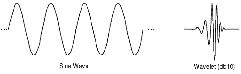
Here illustrated in Figure 4.1 is a comparison between sine wave and one of the

wavelet forms. As the basis function of Fourier analysis, sine wave does not have limited

duration and it is smooth and predictable. On the other hand, wavelets tend to be irregular

and asymmetric. Fourier analysis breaks up a signal into sine waves of various

frequencies. Similarly, Wavelet analysis breaks up a signal into mother wavelet with

different length and position. From this point of view, signals with sharp changes might

Figure 4.1 Comparison of the Sine Wave

As one of the major differences between the Wavelet Transform and Fourier

Transform, the wavelet basis function will be explicitly defined here. The idea behind the

wavelet theory is to define a set of general properties, which the basis function needs to

satisfy in order to be used. This allows for infinite possibilities of basis functions to be

used for the Wavelet Transform, which range from analytical to numerical, orthonormal

or non-orthonormal, etc. The discussion about the properties used to define the wavelet

basis will be presented later in this chapter.

Several families of wavelets that have proven to be especially useful are introduced

here. Notice how these wavelets functions are different in both time and frequency

domain. This fact makes it essential to properly specify, based on what wavelet basis

function the transform was performed, in order to make correct sense of the results. This

wavelet basis is called mother wavelet. The mother wavelet is chosen to serve as a

prototype for all windows in the process. All the windows that are used are the dilated (or

compressed) and shifted versions of the mother wavelet. There are a number of functions

that are used for this purpose. The Daubechies wavelet, the Morlet wavelet and the

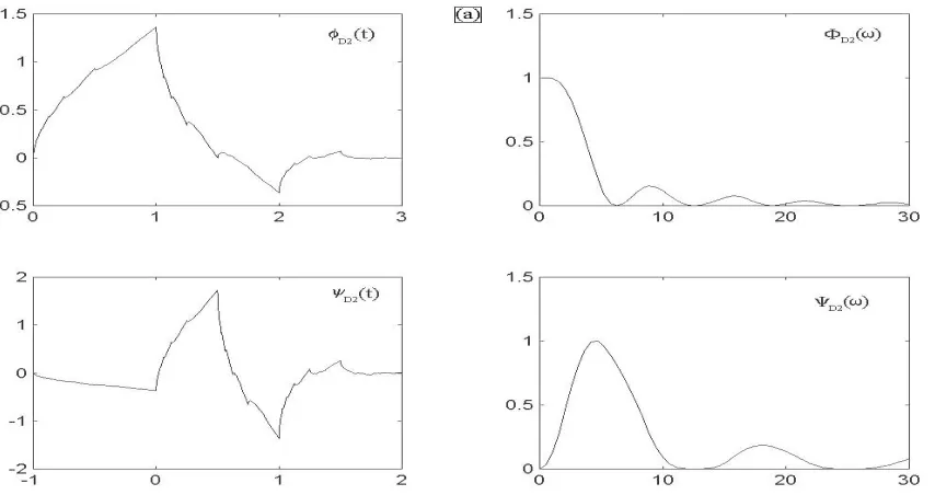
1. Ingrid Daubechies, one of the brightest stars in the world of wavelet research,

invented what are called compactly supported orthonormal wavelets – thus making

discrete wavelet analysis practicable. The name of the Daubechies family wavelets is

written dbN, where N is the order, and db is the “surname” of the wavelet. The

family includes the Haar wavelet, which is written as db1. Figure 4.2 illustrates some

of the scaling and wavelet functions along with their respective Fourier transform for

the Daubechies family.

Figure 4.2 Daubechies wavelets

2. Mexican hat wavelet:

The analytical expression of the Mexican hat wavelet is

( )

14

(

2

)

22

1 3

2 _{x e} x

x − _ − −

  

 

= π

ψ (4.1)

This function is proportional to the second derivative function of the Gaussian probability

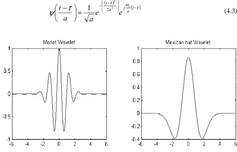
3. Morlet wavelet

Morlet wavelet has [-4 4] as effective support. The analytical equation of it is defined

as:

( )

_{x e} x22_ejω0t

ψ ₌ − _(4.2)

Whereω₀ =1.75π , is selected in order to satisfy one of the wavelet function conditions

[Grossmann, et al, 1989]. Figure 4.3 shows the basic form of the both Morlet and

Mexican hat wavelets. Introducing the scale and translation parameters of the Wavelet

Transform to equation3.2 yields

( )

( )τ ω τ τ

ψ  −

   

 ₋

−

=

    

 − t

a j a t

o

e e

a a

t 2

2

2

1 _(4.3)

Figure 4.3 Morlet and Mexican hat Wavelet forms

4.2 Continuous Wavelet Transform (CWT)

The Continuous Wavelet Transform was developed as an alternative approach to the

is done in a similar way to the STFT analysis, in the sense that the signal is multiplied

with a function, (or the wavelet), similar to the window function in the STFT, and the

transform is computed separately for different segments of the time-domain signal.

However, there are two main differences between the STFT and the CWT:

1. The Fourier transforms of the windowed signals are not taken, and therefore single

peak will be seen corresponding to a sinusoid, i.e., negative frequencies are not

computed.

2. The width of the window is changed as the transform is computed for every single

spectral component, which is probably the most significant characteristic of the

wavelet transform.

4.2.1 Definition

For a signal f

( )

t , the continuous Wavelet Transform is defined as the sum over all

time space of the signal multiplied by scaled, shifted version of the wavelet function ψ:

dt a

b t t f a b a

Wf

∫

+∞

∞ −

∗ _

   

 −

= 1 ( )ψ

) ,

( (4.4)

Where ψ(t): Mother wavelet (* indicates the conjugate)

) (t

f : Signal being analyzed

a: Dilation parameters (a>0)

b: Translation parameters (b∈R)

Herein, the variable a scales the wavelet basis function such that the wavelet function

convolutes with f(t) in different temporal windows, and the variable bacts as a shift

operator by centering the window at several locations. Interpreting in frequency domain,

whether those frequencies are present at a particular stretch of the signal is analyzed by

centering the basis function with the help of variable b. The 1 a factor is used with the

purpose of energy normalization so that, all the scaled wavelets have the same energy

[Rao and Bopardikar, 1998]. The choice of the Mother wavelet is restricted by one of the

most important characteristics-admissibility condition:

∞ < Ψ

=+∞

∫

∞ −

ω ω

ω

ψ d

C

| |

| ) (

| 2

(4.5)

Where

ω ω ψ

ω) (t)exp( i t)d

( = −

Ψ +∞

∫

∞ −

(4.6)

is the Fourier transform of ψ(t).

The results of the CWT are Wavelet coefficients C, which are a function of scale and

position. Multiplying each coefficient by the appropriately scaled and shifted wavelet

can yield the constituent wavelets of the original signals. Here the scale factor, which is

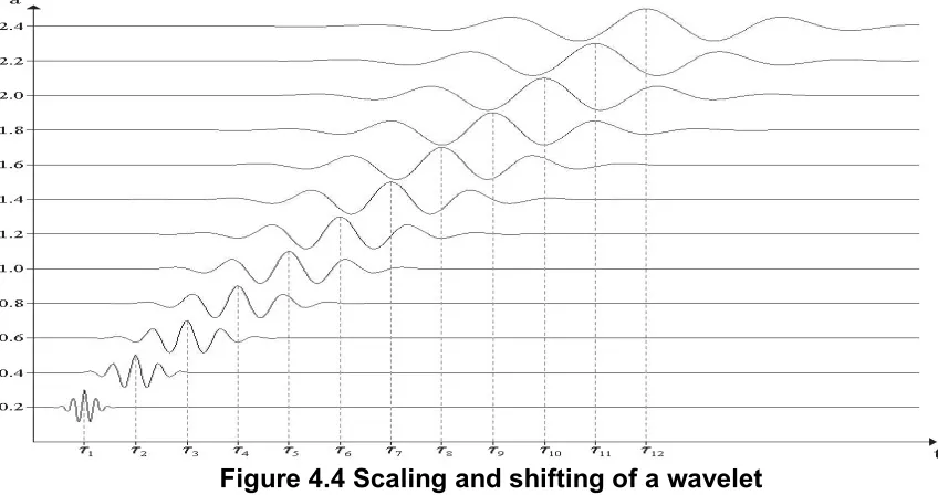
commonly denoted by the letter a, is introduced. Scaling a wavelet simply means to

stretch it. That means the smaller the scale factor, the more compressed the wavelet has

been. It is also clearly shown from the Figure 4.4 that the scale is related to the frequency

Figure 4.4 Scaling and shifting of a wavelet

The use of the scale parameter represents the first difference between the Wavelet

Transform and other types of transforms previously discussed. The result of the Wavelet

Transform of a function yields a two-dimensional time-scale representation by scaling

and translating the window function. Another way to view the Wavelet Transform is as a

decomposition of a function into a linear combination of the wavelets, where the

coefficients )Wf(a,b are the inner products between the function and the wavelet basis

used. By Parseval’s identity, the Wavelet transform can be represented in the frequency

domain, which can be written as:

( )

∫

∞

( ) ( )

∞

− Ψ

= ω ω ω

π

ω _d

e a F

a b a

Wf * j b

2

, (4.7)

Where, )F(ω is the Fourier transform of f

( )

t and _Ψ*

( )

aω _{is the complex conjugate of}

Fourier transform of the mother wavelet. Therefore, the Wavelet Transform can be seen

as a bank of filters with different scales. Here applying the