Approximate analysis of an open multi-class queueing network with class-dependent population constraints

Approximate Analysis

of

an Open Multi-Class

Queueing Network

with

Class-Dependent Population

Constraints

Harry

G. Perras

Y. Dallery

G. Pujalle

Center for Communications and Signal Processing

ElectIical and Computer Engineering Department

North Carolina State University

CCSP TR-89/20

Abstract:

We consider a multiclass open queueing network with class-dependent population constraints. That is, the total number of jobs of each class that maybe present in the network can not exceed a given value. A job that arrives at the network during the time that the current number

of jobs of the same class is equal to the population constraint, is forced to wait in an external

queue. Such queueing networks are especially useful for modelling window-flow control

mechanisms. We present a method for obtaining an approximate solution of such a queueing network. The method is based on the use of an equivalent closed queueing network model, which

is analyzed using an approximate product-form solution technique. The performance parameters of

the original open queueing network are easily derived from the equivalent closed queueing network. Numerical results show that this method is fairly accurate.

Keywords :

Window flow control, open queueing networks, multiple classes, population constraints, performance evaluation, approximate analysis.

1. INTRODUCTION

In this paper, we consider an open queueing network with different classes of jobs and population constraints. With the exception of the population constraints, the basic network we consider is of BCMP type [3]. Each class r of jobs has its own population constraint. That is, the total number of class r jobs that canbe simultaneously present inside the network can not exceed a fixed number, say Nr ·Class r jobs that arrive at the network during the time that there are N, jobs present in the network, are forced to wait in an external queue.As soon as a class r job leaves the network, a job of the same class is allowed to enter the network. Such a queueing network can be

used to analyze the performance of sliding window flow control schemes. For instance, in the case of virtual circuit networks, each virtual circuit has its own end-to-end sliding window flow control. That is, the total number of outstanding unacknowledged packets may not exceed a pre-specified number. A similar window flow control scheme can be found in the OSI protocol for connection oriented traffic, where the total number of unacknowledged TPDU (Transport Protocol Data Units) may not exeed a pre-specified number.

Queueing networks with population constraints do not have product form solutions. (Note that the situation we are considering differs from the case where blocked jobs are lost which leads to product form solutions [22]). As a result, several papers have been devoted to the approximate analysis of open queueing networks with population constraints (OQNs-PC). Most of the approximation methods are based on aggregation techniques. The idea behind aggregation is that a subsystem is replaced by a flow equivalent service center (FESC) with load-dependent service rates [7,24,34]. The service rates of the equivalent server are obtained by analyzing this subsystem in isolation. Theoretical justification of aggregation techniques is provided in two extreme cases: separable networks [2, 12], and nearly completely decomposable systems [14].

The use of aggregation for the analysis of OQNs-PC was originally proposed by Avi-Itzhak and Heyman [1] for networks with exponential servers and a single class of jobs. The aggregation method is as follows. First, we analyze the network without the external queue as a closed queueing network. Let Xc(n) be its throughput for population n, for n

=

1,..., N, where N is the maximumallowable number of jobs in the open network. The networkisthen replaced by an FESC with load-dependent service rates Jl(n) given by : Jl(n) =Xc(min[n, N]), for any n ~ 1.

queueing networks with nested subnetworks, where each subnetwork has its own population constraints [19].

A direct extension of this aggregation technique to the case of networks with several

classes of jobs and class-dependent population constraints was considered by Sauer [33]. The

network, without the external queues, is analyzed in isolation as a closed multiclass queueing

network for all feasible population vectors. The aggregate system is then replaced by a single

queue with service rates dependent on the state vector. This queue is analyzed as a

multi-dimensional Markov chain. This approach can be used for very small models, as it rapidly

becomes very complex due to the total number of combinations that are required to be taken into account. In order to avoid the complexity problem introduced by this approach, several techniques

have been proposed [6, 23, 26, 36].

In

particular, Brandjwan [6] and Lazowska and Zahorjan

[23] independently developed the following method. The system is decomposed into a set of

independent single-class queues with load-dependent service rates, each queue modelling the

behaviour of a particular class of jobs. The load-dependent service rates of a particular class are

obtained by analyzing the closed multiclass queueing network for all population values of this class, while the populations of the other classes of jobs are fixed at their average values. An

iterative procedure is used to determine the load-dependent service rates of each single-class queue.

In addition to the FESC approximation, this method involves an additional approximation which is

due to the assumption that the influence of the other classes on a given class can beadequately represented through the use of average values. A simple approximation technique was proposed

by Thomassian and Bay [36]. This technique is based on the method of adjusted rate [30, 31]. As

in [6, 23], the system is decomposed into a set of single-class FESCs. The load-dependent service

rates of the FESC of a given class are obtained as follows. The original multiclass model is

analyzed as a single-class model. The influence of the other classes is represented by their

contribution to station utilizations. That is, the service rates of this single-class model are obtained

by reducing the service rates of the original network. The FESC is then obtained by aggregating

the resulting single-class network. This approximation technique is very simple since it does not

require the solution of closed multiclass networks. However, as a result of adjusting the service

rates, the performance parameters of a given class are calculated independently of the population

constraints of the other classes, and thismaylead to significant errors.

Multiclass queueing networks with shared population constraint have been considered in [8, 24]. In this case, the total number of jobs (irrespective of their class) that can besimultaneously present in the network may not exceed a pre-specified number. Multiclass queueing networks with

population constrained subnetworks have also been studied in [21]. A simpler case was considered

A different approach for the analysis of OQN-PC has been proposed by Dallery [15]. The model considered in [15] is a single-class open queueing network with general service times. Let N

bethe maximum allowable number of customers in the network. This capacity limitation can be seen as a limited number of resources. Tobeallowed to enter the network, a job needs frrst to get a resource. It will then hold this resource until it leaves the network. Thefirst step of the method is to transform the basic open model into an equivalent closed model. This is done by exchanging the roles of the jobs and the resources. The model obtained is a closed queueing network whose population is equal to the maximum allowable number of customers in the open queueing network. The closed queueing network is composed of the set of stations of the open queueing network plus an additional station which models the external queue. An approximation technique, based on Marie's approximation method [25], is then derived in order to analyze the closed queueing network. The open model can be easily analyzed if we know the solution of the equivalent closed queueing network. It has been shown in [15] that if all service distributions are exponential, then this method provides exactly the same results as the aggregation method. However, in the case of general service times, this method is more accurate than the aggregation method (see [15]). Several extensions of this approach have been considered. In [4], a closed queueing network with general service times and population constrained subnetwork was analyzed. Again it was found that the performance parameters, especially the throughput, were more accurately estimated. In [10], an open multiclass network with general service times and shared population constraints was considered. U sing the above method, this network can be equivalently viewed as a closed multiclass network with a single chain. The behaviour of this closed queueing network was approximated by the behaviour of a closed single-elass queueing network which was then analyzed using the technique presented in [15].

In this paper, we extend the approach proposed in [15] in order to analyze open multiclass queueing networks' with class-dependent constraints. The paper is organized as follows. In section 2, we introduce the open multiclass queueing network with population constraints, and then define the equivalent closed model.

In

section 3, an approximate solution of the closed model is derived. Section 4 deals with the computational procedure for obtaining performance measures of the closed model and subsequently of the original open queueing network. Numerical results are presented in section

5, and,

several extensions are consideredin section 6. Finally, an alternative view of this

approximation method is presentedinthe appendix.

2. THE OPEN MODEL AND ITS EQUIVALENT CLOSED MODEL

We consider an open multiclass queueing network with class-dependent population

constraints. With the exception of the population constraints, the basic network we consider is of

BC~ type [3]. Let M denote the number of service stations and R the number of classes of jobs. Let qO,j(r) be the probability that a class r job joins station j upon arrival at the network, and~/r)

be the probability that a class r job joins station j after service completion at station i. The probability that a class r job leaves the network after service completion at station i, qi,O(r), is therefore given by :

M

qi,O(r) = 1 -

L

qi .(r)

. 1 J

J=

for r

=

1, ..., R (1)

The _rrival process of class r jobs is Poisson withrate

A,..

Each station of the network may beof any BCMP type. Especially, any station, say i, with first-come-first-served (FCFS) service discipline has exponentially distributed service timeswithrate

Jli

independent of the job's class.

In the model consideredin this paper, each class of jobs has its own population constraint Let N, be the population constraint of class r jobs. That is, N_r is the maximum number of class r jobs that can besimultaneously present inside the network. With each class of jobs is associated an external queue. If an r class job arrives while the current number of class r jobs inside the network is less than N_{r ,} it instantaneously enters the network. Otherwise, it has to wait in its external

queue. As soon as a class r job leaves the network, the first-in-line job in the class r external

queue, ifany, enters the system.

The population constraint of each class can berepresented by a set of resources, referred to as tokens. Since the population constraints are class-dependent, each class of jobs is associated

with a class of tokens. The total number of class r tokens is equal to the population constraint of class r jobs, i.e. N_r.Thus,inorder to enter the network, a class r job must firstget a class r token. The job then holds the token during its sojourn through the network. As soon as the job leaves the

network, the token is released and it is immediatly available for another job.

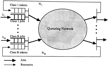
This open model is represented in

figure

1 using the formalism of queueing networks with synchronization introduced in [18]. The internal BCMP network consisting of the M stations is

represented by a circle. Each of these stations

will

bereferred to as aninternal station. There is one external queue per class. The external queue together with the token queue will be referred to as

synchronization station, an assembly takes place and the job/token pair enters the network. When the job leaves the network the t k_{, 0 en IS e}· fi d b_ack Into_{into Its corresponding external queue of}I · resources.

Class 1 tokens

Class R tokens

- - . Jobs ---~~ Resources

Figure 1 : The open model with R classes of jobs

It is quite easy now to see how this queueing network canbeused to model a set of virtual circuits which share the same communication network. The stations of the queueing network can be seen as representing the nodes of the computer communication network, and a job is identified with a data unit upon which the window-flow control is carried out. The path through the queueing network associated with a class of jobs can

be

seen as avirtual circuit, and the maximum allowable number of jobs (i.e, the total number of tokens) canbe identified with the maximum window size of the virtual circuit. Finally, the synchronization station can be seen as the point where the window-flow control is applied.

that is Nr · Therefore, the network is composed of R closed chains of jobs. From this point of

view, the system is a closed multiclass queueing network with external resources (the jobs). The

closed model consists of theMinternal stations of the original network and the R synchronization stations. The number of stations of the closed model is therefore M+R. The M stations of the

original networkare numbered from

1

to

M

and the

R

synchronization stations from

M+1

to

M+R.

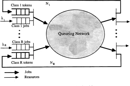
Thus, station M+r is the synchronization station corresponding to therthclass of jobs. Note that this station is visited only by class rjobs, The population vector is N =(N₁, N₂, ..., N_R) .°This

equivalent view is illustratedinFigure 2.

Class 1 tokens

Al

•

•

•

AR

-.

Class R tokens

-~. Jobs

- -...~~ Resources

Figure 2 :The equivalent closed model

Let ..(r) be the routing probabilities of class r jobs in the closed model. These

PI,J

probabilities canbeeasily obtained from those of the open model. We have

pi,j(r)

=

qj.j(r), PM+r,j(r)= qO,j(r), pi,M+r(r) =Cli,o(r),

for i,

j

=

1, ..., M forj

=

1, , M

for i

=

1, , M

(2) (3) (4)

station (station M+r), it is instantaneously served if at least one external resource (i.e. a job) is available. Otherwise, it has to wait until a resource is available, that is until a class r job arrives at the system. Recall that the arrival process of each class of jobs is Poisson. Each time a job (a class r token) is served at station M+r, one external resource (a class r job) is consumed. Note that in the closed model jobs are consumable resources whereas in the open model tokens are non-consumable resources.

It is important to emphasize that the open and closed models are totally equivalent. They differ from each other only by the roles given to the jobs and tokens. Thus, no approximation is introducedin the transformation of the open model into a closed modeL The closed model is just an other way of looking at the same system. Of course, this transformation does not make the problem simpler. In fact, as in the open model, no exact solution of the closed model can be obtained. However, the closed equivalent model is of interest since we can analyze it approximately using known approximation techniques for closed queueing networks, as shown in the next section.

3. APPROXIMATE SOLUTION OF THE CLOSED MODEL

In this section, we extend the technique presented in [15] to derive an approximation solution of the closed modeL This technique is based on Marie's approximation method for general single-class queueing networks [25]. The idea of Marie's method is to replace any non-BCMP station, such as a FCFS station with non-exponential service times, by an equivalent exponential server with load dependent service rates. Thus, the original network is approximated by an equivalent product-form network. The load-dependent service rates are obtained by analyzing each stationinisolation under a state-dependent Poisson arrival process. An iterative procedure is then used to calculate the unknowns. A slightly different view of Marie's method using operational analysis [17] is presentedin [16]. A unified view and a comparison ofproduct-fonn approximation techniques for single-class closed queueing networks, namely the aggregation technique and Marie's method, is presentedin[4].

An extension of Marie's method to queueing networks with different classes of jobs has been proposed in [28]. In general, it is much more complex than in the single-class case. However, in our case, the extension of Marie's method is fairly easy. This is because all the internal stations are BCMP stations. As a result, they do need not to be replaced by an equivalent station. The only non-BCMP stationsarethe synchronization stations. Now, each of these stations is visited only by a single class of jobs. Therefore, the equivalent station is simply obtained as in

The closed model is thus approximated by a multiclass closed queueing network of BCMP type. This equivalent network has M+R stations, the M internal stations (stations 1 to M) and R single-class exponential stations with load-dependent service rates (stations M+ 1 to M+R). It is

illustrated in figure 3. Obviously, the

R

classes of jobs form a set of

R

closed chains. Since the

equivalent network is ofBCMP type, the routing of each class of jobs is characterized only by the

average visit rates. Let Vi(r)

be the average visit rate of class r jobs at station i, i.e., one of the

solutions of the following systemof

M+1

equations

[3] :

M

Vi(r)

=

j~l

Vj(r) Pj,i(r) + VM+r(r) PMff,i(r) for i

=

1, ..., M and i

=

M+r (5)

The solution of (5) is determined up to a multiplicative constant. We choose the solution such that

V

M+r(r)

=

1.

Then, Vi(r) can be interpreted as the average visit rate of a class r job at station

i

between two consecutive visits at the synchronization station. Also, it

is

easy to check that the

average visit rates are equal to those of the open model.

Closedchain

1 : N1

customers

Class

1

external station

•

•

•

Class R external station

Closed

chain R : N

R

customers

Figure 3 : The approximate closed queueing network

10

•

•

Let ~M+r(n)bethe load-dependent service rate of the rth equivalent station when n jobs (tokens) are present at this station. Recall that this station corresponds to the synchronization station of class r jobs. We now show how these parameters can be determined. This procedure is similar to that used in the case of single-class networks. Therefore, some of the details will be omitted and the interested reader is referred to [4, 15, 16,25]. As proposed by Marie [25], the parameters of each equivalent station are obtained by analyzing the corresponding station in isolation fed by a state-dependent Markov arrival process. Let us consider therth synchronization station, that is station M+r. Let A.M+r(n) be the state-dependent rate of the Markov arrival process when n jobs (tokens) are present at the station. The model of this synchronization station in isolation is shown in figure 4.

Class r tokens (jobs) A. (n)

M~

Classrjobs (resources)

Figure 4 : Analysis of classr synchronization station in isolation

The steady-state solution can be easily obtained ([15], [19]). Letp~+r(n)bethe

steady-state probability of having n jobs (tokens) in the class r synchronization station when considered in isolation. Then, the conditional throughputs, vM+r(n), can beobtained as [25] :

I

. PM+r(n-l)

v

_M (n)

=

~+r(n-l) I

+r PM+r(n)

for n

= 1, ..., N_r

(6)

The conditional throughput is the inverse of the pseudo service time used in [15, 16]. The pseudo

° tim

S

(0) - l/v (n) is the expected time station

M+r

spends in state

n

between two

semce e, M+r - M+r '

consecutive completions occuring while the state is n. Then, it was shown in [15] that the

conditional

throughputs are given by :

I

vM+r(l)

=

1 1

A

_r ~+r(O)

for n

=

2, ... , N,

(8)

The synchronization station is then replaced by an equivalent station having load-dependent service rates equal to the conditional throughputsin isolation[25], i.e. :

for n= 1, ..., N,

(9)

The analysis of a stationinisolation requires the knowledge of the state-dependent arrival rates. Actually, in the case of a synchronization station, only the quantity AM+r(O)is required. These quantities are obtained from the product-form solution of the equivalent BCMP network [25]. Indeed, provided that the load-dependent service rates of all equivalent stations are known, the resulting BCMP network can be solved exactly. Especially, the marginal probabilities of each equivalent station can be obtained. Let PM+r(n) be the steady-state probability of having n jobs at the rth equivalent station, i.e., station M+r,in the equivalent network. Then, the state-dependent arrival rates are obtained as [16, 25] :

for n =0, ..., N_r-l (10)

Note that equation (10) is a reverse form of equation (6). Actually, equations (6), (9), and (10) imply that the marginal probabilities of each equivalent stationinisolation and inside the network are equal, i.e, pIM+r(n)

=

PM+r(n).

As it appears, the load-dependent service rates of the equivalent stations depend on the state-dependent arrival rates (through the analysis of each station in isolation), which in tum depends on the load-dependent service rates (through the analysis of the equivalent network). Therefore, an iterative procedure must be usedinorder to determine the unknown parameters. This

procedure is presented in the next section.

4. ALGORITHMIC SOLUTION

The solution presented in section

3

is obtained by approximating the closed model by an equivalent BCMP network. This network is a multichain closed queueing network consisting of M+R stations and R classes of jobs with population vector is N = (Nj, N2, ... ,NR) · The only

unknown parameters of this network are the load-dependent service rates of each of the R single-class equivalent stations. Now, some of these parameters are easily obtained. In particular, from

equations (8) and (9), we have:

JlM+r(n)

=

~ for all n

=

2, ..., N, and r = 1, ..., R (11)

Therefore, the only unknowns are the quantities JlM+r(I), for r=I, ...,R. These parameters can be obtained as the solution of the following fixed-point problem. Let us suppose for a moment that we know these quantities. Then, we can solve the closed queueing network using any computational algorithm, (such as the convolution algorithm [9, 11]), in order to obtain the marginal probabilities of each equivalent station, PM+r(n). Using these probabilities, we can calculate the state-dependent arrival rates AM+r(O) from equation (10). (Note that only the probabilities PM+r(I) and PM+r(O) are needed.) Also, the conditional throughputs vM+r(l) can be calculated using equation (7). Finally from equation (9), we can obtain a set of new values for the load-dependent service rates which can be used in the next iteration to solve the closed queueing network. We can thus iterate until convergence of the load-dependent service rates. We note that we can directly express the unknowns as a function of the steady-state probabilities of the closed queueing network. That is, using equations (7), (9), and (10), it is easy to show that:

(12)

Thus, the following simple iterative procedure can then be used to solve this fixed point problem.

Computational Algorithm

Initialization step :

Set JlM+r(l) =

Ar,

for all r = 1, ... , R.

Iteration step :

Step 1. Solve the closed queueing network with the current values ofJ.1M+r(1),r=1,...,R. Step 2. Calculate new values of the load-dependent service rates, J.1M+r(1), for all r=l,...,R,

using equation(12).Goto step 1 until convergence of the quantities J.1M+r(1)· •

Let us now discuss the computational complexity of this approximation technique. Obviously, its computational complexity is relatedtothe solution of the multiclass BCMP network

in step

1.

Ifthe above algorithm is applied without any particular care, its computational burden

iterations differ only from each other by the parameters of the R equivalent stations. This

observation can be used to drastically reduce the computational complexity as discussed below.

At each iteration of the algorithm, the closed queueing network, say C, has to besolved using the latest updated values of the quantities J..lM+r(l). Now, let

cr

be the closed queueing network obtained from C by removing the rth equivalent station, that is station M+r. Thus, this network consists of the M internal stations and the R-l synchronization stations corresponding to all classes but class r. Let Xr(N) bethe throughput of class r jobs in network

cr

with population vector N

=

(NI , N2, ... , NR) . Then, using classical formulae of product-form networks [9], it

is easy to show that :

=

(13)

So, what has to becalculated are the quantitiesXr(N),for allr. Now, suppose that we use the convolution algorithm [9, 11] to analyze network

cr.

As it is known, the convolution algorithm calculates the normalizing constants of the network from which the performance parameters,

especially the throughputs, can be easily derived. These normalizing constants are calculated recursively starting with one station and step by step incorporating the other stations, one at each step. Each step consists of a convolution operation. Let us now see how this algorithm can be applied to network

cr

assuming that the recursion is petformed in the orderin which the stations are numbered. After M-l steps (convolution operations), we get the normalizing constants corresponding to the internal network, say CI , consisting of the M internal stations. The

normalizing constants of network

cr

are then obtained by performing R-l additional convolutions corresponding to the synchronization stations. Now, the following points must be emphasized. First, the last R-l convolutions involve only single-class stations. Therefore, the major computational complexity is related to the M-l convolutions required to obtain the normalizing

constants of network

e

I . Secondly, since all networks

cr

have the same internal network

CI,

the normalizing constants of

e

I _{need only be calculated once. Finally, since the internal network}

CI

remains the samefor

all

iterations, the normalizing constants of

CI

need only becalculated once at the first iteration. So, by taking into account these observations, the computational complexity of

the algoritm may be significantly reduced. Indeed, it reduces to calculating the normalizing

constants of networkCl once, and then at each iteration, performing convolutions with single-class

stations.

Thus, the computational complexity of the approximation technique is mainly that of

algorithm. This is feasible for networks of moderate size. However, for large networks, this may no longer be feasible since the computational time and space requirements of exact algorithms such as the convolution algorithm grow very rapidly with the size of the network, i.e., number of stations, number of chains, population vector. Insuch cases, some sort of approximation has to be used to solve the equivalent BCMP network and get the values of XT(N) for all r. Many approximation algorithms, mainly based on the MV A algorithm [32] have been proposed for solving BCMP networks (see among others [13, 35, 39]). Now, the R equivalent stations have load-dependent service rates. Therefore, we need an approximation technique that can handle such service stations. Most of the proposed techniques do not allow stations to have load-dependent service rates. There are however some which do [20, 27, 38]. These techniques can then beused to calculate an approximate value of the throughput XT(N) of each network

O.

It is important to notice that the equivalent network has a particular structure. Inparticular, the only stations that have load-dependent service rates are single-class stations, Le., they are visited only by one class of jobs. Moreover, the load dependence has also a special form: all the service rates but the first one are identical, i.e.

(14)

These two features may be useful to derive an efficient approximation technique for solving the equivalent network. (This issue was not investigated as it is beyond the scope of this paper.)

Finally, we note that using (13), equation (10) implies:

Then, using (7), (9), and(15), the conditional throughput can be expressed as :

1

~+r(1) = 1 1

----

A

Xr(N) r

(15)

(16)

This expression can be equivalently used in step2of the algorithm instead of equation (12), in

order to calculate updated values of the conditional throughput

~M+r(1)·

tokens QTi(r) at station i, can be calculated for any internal station as well as for the class r synchronization station. Now, the performance parameters of the open model are easily obtained using the equivalence between the two models. Let XJi(r) and QJi(r) denote the throughput and mean number of class r jobs at any internal station i. Since inthe internal network jobs and tokens

areidentical, the performance parameters pertaining to jobs in the open model are identical to those pertaining to tokens in the closed mooel. This holds for all internal stations. Therefore, we have

for i

=

1, ..., M (17)

Consider now the external queue. Let XJe(r) and QJe(r) denote the throughput and mean number of class r jobs at the external queue. From the analysis of the synchronization station, it is easy to show that [15] :

J 1

Q /r) = PM+r(O) A ''M+r(O)

- 1

A

_r

(18)

(19)

Little's law can then beused to derive the mean time (or mean response time) of each class of jobs at any internal station and at the external station :

fori

=

1, ..., M (20)

(21)

Finally, the mean system time of a class r job, i.e., the average total time a job spends in

the system, is given by :

M

RJ(r) = RJe(r)

+

L

Vj(r) RJj(r)

i

=

1

The proposed approximation technique for the analysis of the original open model is mainly based on the analysis of its equivalent closed model. A different, yet equivalent view, of this approximation technique is presented in the appendix. The reason for presenting this

alternative view is that it can provide a different insight to the proposed technique. Finally, we note that in the case of single-class jobs, the technique presented in this paper reduces to the technique

presented in [15]. Furthermore, for single-class BCMP networks, it is equivalent to the aggregation method In this special case, the algorithm does not require any iterations.

5. NUMERICAL RESULTS

In this section, we discuss the accuracy of the approximation algorithm presented in section 4. The algorithm was implemented on a SUN workstation. The approximation results were then compared to simulation results obtained using the simulation features of QNAP2[37]. Validation results are given for the two queueing networks shown in figure 5 and 11.

The queueing networkin figure 5 consists of three stationsin tandem and three classes of jobs. Each station is represented by a circle, and it is assumed tobe a single server queue with an exponentially distributed service time. For each class, the arrival process of jobs is assumed tobe Poisson distributed. The routing of each class is shown by the means of a continuous line.

'-!'IIIJ-.2.IIIJ

~IIIJ-Figure 5: Three stations withthreeclasses

This particular configuration was analyzed assuming that a) all three classes are

symmetrical, i.e.

Nl=N2=N3=N,

and

Al=A2=A3=A and

b) the three classes are not symmetrical, i.e.each clas r,r=1,2,3, has a different N

r

and a different arrival rate

Ar.

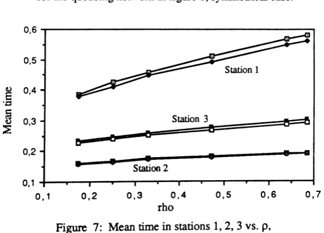
The performance measure used in all comparisons is the mean waiting time in each station.Infigures 6 and 7, we give the

approximation and simulation results for the mean time in an external queue, and the mean time in

stations 1, 2, and 3, for the symmetrical case. These results are plotted as a function of the utilization

p

of the external queue, i.e. the percent of time the queue is not empty. Simulation

simulation results are very clo_{. se.}Th_{e resu ts were obtained}I . _{by varying the arrival rate}

A

_{from 2.0} to 2.42 while N=3 and Jll= 8, Jl2= 12, Jl3= 10.

0,7

0,6

0,5

0,2 0,3 0,4

rho

Figure 6: Mean time in external queue vs.

p,

for the queueing networkinfigure 1, symmetrical case.

I:

O-r----,-..,..-r--r--r---r-,-~-...----.~ ...--J

0,1

2

3,---

____

0,7 0,8

0,5

0,2 0,3 0,4

rho

Figure 7: Mean timein stations 1, 2, 3 vs.

p,

for the queueing network infigure 1, symmetrical case.

0,6

0,5

0 _0,4

e

..0

~

0,3

~

0,2

0,1 0,1

The non-symmetrical case of the queueing

network

shown in figure

5

is reported in figures

8, 9,

and

10.

In particular, in figure

8 ,

we give the approximate and simulation results for the mean time in the external queue of class

1

as

a

function of the utilization

PI

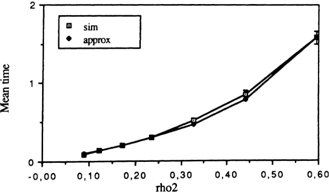
of the external queue. Similar results are given for class 2 in figure 9 as a function of the utilization

P2

of the class

that of class 2.) In figure 10, we give the approximate and simulation results of the mean time in station I, 2, and 3 for class 1 as a function of the utilization

PI

of the class 1 external queue. Simulation confidence intervals are given only in figures 8 and 9, seeing that in figure 10 the

approximate and the simulation results are very close. The results were obtained by varying the arrival rates from (Al,A2,A3)=(1.3,1.8,2.3), to (Al,A2,A,3)=(1.9,2.4,2.9). (Nl,N2,N3) = (2,3,4),

and J.ll= 8,

Jl2=

12, ~3= 10.

12

10

1=

sim

8

Q)

E

':::2 ₆

~

~ 4

2

a

0,00 0,20 0,40 0,60 0,80 1 ,00

rho I

Figure 8: Mean time in class I external queueVS. PI,

for the queueing network in figure 1, non-symmetrical case.

2~---,

I :

0,60 0,50

0,40 0,10

o..L----.-::..--~--'T'--r--__,r---,--r-....,..-.,---,.-..,

-0,00 0,20 0,30

rho2

Figure 9: Mean time in class 2 external queue

VS·P2,

for the queueing network

in

figure 1, non-symmetrical case

0,6

0,5

0 _0,4

E

..0

~

0,3

:E

0,2

0,1 0,00

Station 3

nO ~

~--fF

&:= _{Station 2}

•

•

•

.

-

• •

0,20 0,40 0,60 0,80 1,00

rho 1

Figure 10: Mean time in station 1,2,3 for all classes vs. PI,

for the queueing networkinfigure 1, non-symmetrical case.

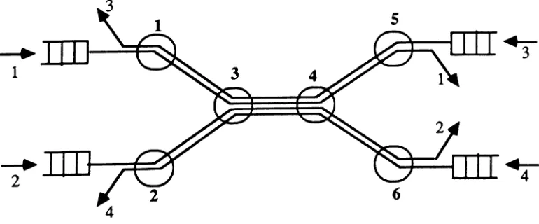
Similar experiments were carried out for the queueing network shown in figure 11. The queueing network consists of six stations and four classes of jobs. As before, each station is represented by a circle, and it is assumed to be a single server queue with an exponentially distributed service time. For each class, the arrival process of jobs is assumed to bePoisson distributed. The routing of each class is shown by the means of a continuous line. This queueing network was analyzed under a) the symmetrical case, where Nr=N and

Ar=A

for r=I,2,3,4, and b) the non-symmetrical case, where each class r, r=I,2,3,4, has a different N, and a different arrival rate

A

r . For simplicity, it was assumed that stations 1, 2, 5, and 6 have the same service rate.

Also, stations 3 and 4 were assumed to have the same service rate.

--.

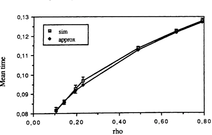
₁

In figures

12, 13

and

14,

we give the approximation

and

simulation results for the mean

time in an external queue, the mean time in station3(which is identical to that in station 4), and the mean time in station

1

(which is identical to that in stations 2, 5, 6), for the symmetrical case.

These results are plotted as a function of the utilization of the external queue. The results were

obtained by varying the arrival rate from

4.5

to

5.8,

while

N=5, and

J.11=J.12=J.15=~=14, Jl3=~=

30.

3~---...,

0,80 0,60

0,20

sim

1=

0,40

rho

Figure

12:

Mean timeinexternal queue vs.

p,

for the queueing networkinfigure 7, symmetrical case.

2

0.J----I1I::::::!~..;p.--..--...,...-_..,r___-~---,~-,

0,00

0,13

0,12

I :

.~

0,11

fi

0,10

::E

0,09

0,08

0,00 0,20 0,40 0,60 0,80

rho

Figure 13: Mean

time in

station 3

vs.

p,

for the queueing network

in figure

11,

symmetrical

case.

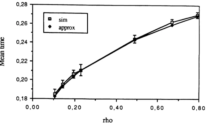
0,28

0,26

I :

.g

0,24

~

0,22

::;

0,20

0,18

0,00 0,20 0,40 0,60 0,80

rho

Figure 14: Mean time in station 1 vs. p,

for the queueing networkin figure 11, symmetrical case.

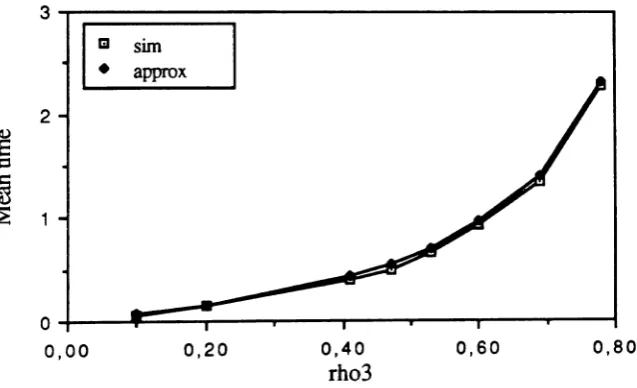
The non-symmetrical case of the queueing network shown in figure 11 is reported in figures 15, 16, and 17. Infigure 15, we give the approximate and simulation results for the mean time in the external queue of class 1 as a function of the utilization

PI

of the external queue. Similar results are given in figure 16 for class 3, as a function of the utilization

P3

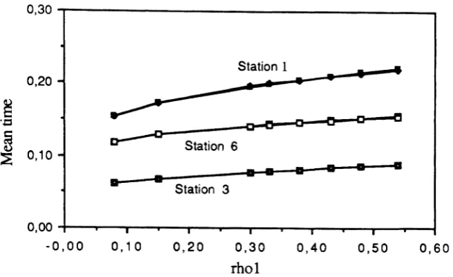
of the class 3 external queue. (The error of the approximate results for the external queues of class 2 and class 4 is similar to that for class 3.) In figure 17, we give the approximate and simulation results of the mean timein station 1, 3, and 6 for class 1 as a function of the utilization

PI

of the external queue of class 1. These results are representative of the type of results obtained for each class. Simulation confidence intervals are given only in figures 15 and 16, seeing that in figure 17 the approximate and the simulation results are very close. The results were obtained by varying the arrival rates from (A,1,A,2,A,3,A,4)=(5,4,3,2), to (AI,A2,A3,A4)=(6.5,5.5,4.5,3.5). (N1,N2,N3,N4)=(5,4,3,2) and JlI=Jl2=JlS=Jl6=14, Jl3=JJ,4=30.

0,60 0,50

0,40 0,10 0,20 0,30

rho1

Figure 15: Mean time in class 1 external queue vs. PI, for the queueing network in figure 11, non-symmetrical case

0,00 ;--r----r---.--....--r---...-....--...---P"-...-~

-0,00 0,80

EI _sim

0,60

•

~

.g

0,40

~

:s

0,20

3

I:

siro

2

~

E

-::1

~

~

0,80 0,60

0,20

O.+----..111~---.---..,----r---y----,--~---1

0,00 0,40

rho3

0,30 . , . . . - - - _

Station 1

~:

:

0,20

•

~

0::i

e--CF 0

~

_0,10 Station 6

~

• •

• • •

•

..

•

_{Station 3}

0,00

-0 ,00 0,10 0,20 0,30 0,40 0,50 0,60

rho 1

Figure 17: Mean time in stations 3,1, and 6 vs. PI,

for the queueing network in figure 11, non-symmetrical case

In general, it appears that the performance parameters of the internal stations are always very accurately estimated (see figures 7, 10, 13, 14, and 17). The accuracy of the results corresponding to the external queues depends on the load of the system. A fairly good measure of

the load of the system is provided by the percentage of time each external queue is non-empty, referred to as the utilization of the external queue. This utilization increases when either the arrival

rate increases or the window size decreases. Let us first consider the case where all classes are symmetrical. For these cases, when the load increases (as a result of the increase of the arrival rates), the error increases (see figures 6 and 12). Similar observations were made in the case of

single-class networks. Now, in the non-symmetrical cases, the difference in the accuracy of the

results pertaining to different classes may besignificant (compare figures 8 and 9, and 15 and 16). In general, it seems that for reasonable loads of the system, the proposed method has a satisfactory

accuracy. Its accuracy is comparable to the one obtained in the case of single-class networks.

On all the examples we tested, the algorithm always converged. The convergence can actually formally be proved in the special case of two classes of jobs. The number of iterations

required to achieve a reasonable accuracy is of the order of 10, and it increases as the load of the

6. EXTENSIONS

In this section, we briefly discuss several extensions of the method presented in this paper. These extensions are discussed independently of one another, but they can easily be combined.

Afirst extension is related to the feedback of tokens. So far, it was assumed that a token is immediatly available upon departure of a job. This may not be the case in real systems. The algorithm can be easily extended to allow a non-zero delay for the return of tokens. For instance, tokens may go back following the reverse path of the jobs, or following a different route.With this additional assumption, the equivalence between the open and closed models still holds, but the average visit rates of tokens differ from those of jobs. In particular, let yTi(r)bethe average visit rate of class r tokens at station i, and let yJi(r) bethe average visit rate of class r jobs at station i. It can be easily shown that: yTi(r) ~ yIi(r). The closed model can thenbe approximately analyzed using the method presented in section 4. Note that since the jobs of the closed model are the tokens, the average visit rates of the closed model are those corresponding to tokens, i.e, yTi(r). Let QTi(r) and RTi(r) denote the mean queue length and mean response time of class r tokens at

station i in the closed model. Then the performance parameters of the open model can again be derived. Let XJi(r), QIi(r), and RJi(r) denote the throughput, mean queue length, and mean

response time, of class r jobs at station i, respectively. Then, we have

J

1 Y i(r) T

Q

.(r) = -

Q

.(r)

1 y~(r) 1

1

fori = 1, ..., M

fori=I, ...,M

fori = 1, ..., M

(23)

(24)

(25)

Finally, the mean system time ofa class rjob,RI(r),is

M

RJ(r)

=

RJe(r)

+

L

VJi(r) RJi(r)

i

=

1

(26)

A second extension that can be handled by the approximation algorithm, is to allow the

external arrival process of any class to

be

state-dependent, Let

Ar(.) be

the rate at which class r jobs

arrive. Two cases may be considered. First, this rate may depend on the total number of class r jobs n currently present in the system, i.e. either inside the network or waiting in the external

queue. This type of state-dependency can be used to model a finite source of jobs. In that case

~(nr)

=0 for

~ ~

K,

where

K,

is the population of class r jobs. Secondly, this rate may depend

only on the total number of jobs currently present in the external queue, lIly..This can be used to model, for instance, a [mite buffer capacity of the external queue. In that case ~(lIly.) = 0 for lIly.~

Br , where

B,

is the capacity of class r external queue. That is, a job arriving while the external

queue is full is lost. Incorporating the above two types of state-dependent arrivals in our approximation method is very easy, as it only needs to sligthly modify the analysis of the individual synchronization stations. (For details see [4].)

A third extension is to incorporate open classes of jobs without population constraints as well as closed classes of jobs. That is, in addition to the R open classes with population constraints, there are also

Ro

open and Rc closed classes of jobs. First, the effect of the

Ro

open classes of jobs can be taken into account by reducing the service rates of the stations using the method of adjusted rate [30, 31]. Although this transformation is not exact since the original network is not BCMP (due to the population constraints on the other R open classes), it usually provides very good results. Now, we end up with a network with R open classes with population constraints and R_c closed classes. In a similar way as we did in section 2, we can define an equivalent closed model. This model consists of R+Rc closed chains of jobs: the R classes of tokens and the

Rc

classes of jobs. An approximate solution of this closed model can be obtained with the method presentedin sections 3 and 4. The only difference is that the equivalent network has

Rc

extra classes of jobs. Note that there are still only R equivalent stations.

A fourth extension is to allow some classes of jobs to share the same population constraint. This maybeobtained by combining the treatment of open multiclass queueing networks with shared constraints as proposed in [10] with the method presented in this paper. The idea behind this extension can beeasily presented by the means of an example. Let us consider a system with 4 classes of jobs. Classes 1 and 2 share the same population constraints, N1-2' That is, the total number of class 1 and class 2 jobs inside the network can not exceed N1-2'A class 1 (or class

2) job arriving in the system while there are already N1-2jobs of class 1 or 2 is forced to wait in an external queue. This queue contains all jobs of classes 1 and 2 waiting to enter the network. Then, when a job of either class 1 or class 2 leaves the network, the first jobin the external queue is allowed to enter the network. Similarly, we assume that classes 3 and 4 share the same population constraint, N

3-4. The open model can again be transformed into an equivalent closed model.

However, this closed model is slightly more complicated as it consists of 4 classes of jobs but only 2 closed chains. Chain 1-2 (respectively 3-4) has a constant population NI -2 (respectively N3-4) '

model can then be transformed into a closed model with two chains and two classes of jobs. Again, although this transformation (aggregation of classes within each chain) is not exact since the closed network is not BCMP (due to the synchronization stations), it should only introduce a

moderate error. The resulting closed network can again be analyzed with the method proposed in section 3 and 4. The performance parameters of the original open network can then be derived. (For details see [10].)

Finally, we mention that it may be possible to incorporate non BCMP stations in the original network, for instance FCFS exponential stations with class-dependent service times or

REFERENCES

[1] B. Avi-Itzhak and D.P. Heyman, Approximate queueing models for multiprogramming computer systems, Operations Research 21, pp. 1212-1230,1973.

[2] S. Balsamo and G. Iazeolla,

An

extension of Norton's theorem for queueing networks, IEEE Trans. on Soft. Eng., SE-8, pp. 298-305, 1982.

[3] F. Baskett, K.M. Chandy, R.R. Muntz, F. Palacios-Gomez, Open, closed and mixed networks of queues with differents classes of customers, J. ACM 22 N° 2 pp. 248-260

April 1975. " ,

[4] B. Baynat and Y. Dallery, On product-form approximation techniques for general closed queueing networks, Tech. Rep. MASI, in preparation.

[5] A. Brandwajn, A model of a time sharing virtual memory system solved using equivalence and decomposition methods, Acta Informatica 4, pp. 11-47, 1974.

[6] A. Brandwajn, Fast approximate solution of multiprogramming models, Perf Eval. Rev. 11, pp. 141-149, 1982.

[7] A. Brandwajn, Equivalence and decomposition in queueing systems :

a

unified approach, Performance Evaluation 5, pp. 175-186, 1985.

[8] A. Brandwajn and W. M. McCormack, Efficient approximation for models of multiprogramming with shared domains, Perf. Eval.Rev.,pp. 186-194, 1984.

[9] S.C. Bruell and G. Balbo, Computational algorithms for closed queueing networks, Operating and Programming Series, Vol. 7, North Holland, 1980.

[10] B.N. Bui and

Y.

Dallery, Approximate solution of open multiclass queueing networks with general service times and shared population constraint, Tech. Rep. MASI,inpreparation.

[11] J.P. Buzen, Computational algorithms for closed queueing networks with exponential servers, Comm. ACM 16,9, pp. 527-531, Sept. 1973.

[12] K.M. Chandy, U. Herzog, and L. Woo, Parametric analysis of queueing networks, IBMJ.

Res. and Develop. 19, pp. 36-42, 1975.

[13] K.M. Chandy and D. Neuse, Linearizer : a heuristic algorithm for queueing network models of computer systems, Comm. ACM, Vol. 25, N°2, pp. 126-134, 1982.

[14] P.J. Courtois,Decomposability: queueing and computer applications, Academic Press, New York, 1977.

[15]

[16]

[17]

[18]

Y. Dallery, Approximate a~alysis of gener~ open queueing networks with restricted capacity, Tech. Rep. LAG, N 87-08, 1987,

revised

February 1989.

Y. Dallery and X. Cao, Operational analysis of stochastic queueing networks, Tech. Rep. MASI, N°252, September 1988.

P.l. Denning and J.P. Buzen, The operational analysis of queueing network models, Computing Surveys 10,

n?

3, pp. 225-262, 1978.

N°3, pp. 187-196, 1986.

[19] S. Fdida, H. Perros, a!1d A. Wilk, Semaphore queues: Modelling multi-layered window flow co~trol mechanisms, Tech. Rep. MASI, N°181, Mai 1987, to appear in IEEE

Transactions on Communications.

[20] A. Krzesinski and J. Greyling, Improved linearizer methods for queueing networks with queue dependent centres, ACM Sigmetrics Conference, 1984.

[21] A. Krzesinski and P. Teunissen, Multiclass queueing networks with population constrained subnetworks, Perf. Eval. Rev. 13, pp. 128-139, 1985.

[22] S.S. Lam, Queueing networks with population constraints, IBMJ.Res. and Devel. 21 pp.

370-378, 1977. '

[23] E.D. Lazowska and J. Zahorjan, Multiple class memory constrained queueing networks,

Perf. Eval. Rev. 11, pp. 130-140,1982.

[24] E.D. Lazowska, J. Zahorjan, G.S. Graham, and K.C. Sevcik, Quantitative system

performance: computer system analysis using queueing network models, Prentice Hall, 1984.

[25] R. Marie, An approximate analytical method for general queueing networks, IEEE Trans. on

Software Engineering, SE-5, n?5, pp. 530-538, Sept. 1979.

[26] D.A. Menasce and V.A.F. Almeida, Operational analysis of multiclass systems with variable multiprogramming level and memory queueing, Computer Performance 3, 3, pp. 145-159, 1982.

[27] D. Neuse and K.M. Chandy, SCAT: A heuristic algorithm for queueing network modelsof

computing systems, ACM Sigmetrics Conference, Las Vegas, September 1981.

[28] D. Neuse and K.M. Chandy, HAM : The heuristic aggregation method for solving general closed queueing network models of computer systems, ACM Sigmetrics Conference, Washington, September 1982.

[29] R. Onvural, H.G. Perros, and U. Koerner, On a multi-class queue with class dependent window-flow control, Proc. Modelling Techniques and Tools for Computer Performance Evaluation, Palma de Mallorca, Spain, Sept. 1988, pp 245-264.

[30] M. Penottiand M.Schwartz, Congestion control in a store-and-forward tandem links, IEEE

Trans. on Communications, COM-23, pp. 1434-14443, 1975.

[31] M. Reiser, Performance evaluation of data communication systems, Proceedings of the

IEEE,

Vol. 70, N°2, 1982.

[32] M. Reiser and S.S. Lavenberg, Mean value analysis of closed queueing networks,JACM

27, n? 2, pp. 313-323, 1980.

[33] C.H. Sauer, Approximate solution of queueing networks with simultaneous resource

possession,

IBMJ.Res. and Develop.

25, pp. 894-903, 1981.

[34] C.H. Sauer and K.M. Chandy,

Computer systems performance modelling,

Prentice-Hall,

1981.

Stochastic Control and Optimization, Amsterdam, 1979.

[36] A. Thomassian and P. Bay, Analysis of queueing network models with population size constraints and delayed blocked customers,Perf. Eval. Rev., pp. 202-216, 1984.

[37] M. Veran and D. Potier, A portable environment for queueing systems modelling, INRIA Report, N°314, 1984.

[38] J. Zahorjan and E. D. Lazowska, Incorporating load dependent servers in approximate mean value analysis,ACM Sigmetrics Conference, 1984.

APPENDIX

In this appendix, we briefly present an alternative view of the approximation technique

proposedin this paper. Consider again the open model defined in section 2 and illustrated in figure 1, and let us consider the input process of class r jobs to the internal network. This input process is

also the output process of the external queue of class r jobs. Because of the population constraint (at most N, jobs of class r canbe inside the network), this process is no longer Poisson (in fact it is not a renewal process either). Obviously, this process is dependent on the state of the internal

network. So, the idea is to approximate this process by a state-dependent Poisson process.

•

Let

A.

_r(k.)bethe arrival rate of this process given that there are

k,

jobs of class r inside the

network. Let us now characterize these rates. When there are already N, class r jobs inside the

network, this input process is interrupted. Therefore,

(AI)

On the other hand, when there are strictly less than Nr-l class r jobs inside the network,

there are at least two tokens available and therefore, a new class r job arriving from outside (according to the Poisson process with rate

A

_{r )} will instantaneously be allowed to enter the network. As a result, we have:

for all~<Nr-I (A2)

Now, the case where k, = Nr-I, i.e., there is exactly one token available, is more

involved.In this case, the rate depends on whether the external queue of jobs is empty or not at the instant of transition into state

k,

=

Nr-I. Ifit is empty, then the rate is equal to the arrival rate of jobs, i.e.

A.r

Otherwise, the rate is infinite since there is at least one job and one token available. So, the rate "';(Nj-I) is a weighted average of these two rates. Especially,it is such that:

"-r

<

'" • (Nr-l)

<

00. In order to determine this rate, it is convenient to use the following conservation of

. r

flow equation :

(A3)

*

where

P,

(k.)is the steady-state marginal probability of havingley.jobs inside the network. The left

hand side of equation (A3) is the average input rate to the inside network. Provided that the system is stable, it is equal to the arrival rate of jobs into the system, i.e.

A,..

Now, using (AI), (A2), and (A3), after some manipulation we get:

(A4)

Following this approach, the open model can be approximated by an open queueing network which is again of the BCMP type. It consists of M internal stations and R open chains

•

with state-dependent arrival rates. The unknown parameters are now the quantities

A

_r(Nr-I) for all

•

r. Since they depend on the probabilities Pr

<lcr)

which in tumdepend on these parameters, they can

be determined using aniterative procedure.

We now show that this approach is equivalent to that presented in the main part of this paper. It is well known that the above open queueing network with state-dependent arrivals can be

transformed into anequivalent closed network by modelling each external arrival process by an additional station. The resulting closed network consists of the M internal stations plus the R

external single-class stations modeling the arrival of jobs. It has R closed chains. Again, let M +r

•

denote the index of the rth external station. Let_'M+rLL - (n) be its load-dependent service rate. Then,

we have

•

•

Jl_M+r(n) =

A

_r(Nr-n) for n = 1, ..., N, (A5)

Thus, we end up with a closed queueing network that has the same structure as the one consideredin section 3.Inorder to show that these two networks are the same, it suffices to show

•

that the service rates of the equivalent stations are defmed in the same way. Let PM+r(n) bethe

steady state probability of the rthexternal station.Then

•

•

PM+r(n)

=

P (Nr-n)r for n

=

1, ...,N, (A6)

*

~M+r(n)

=

J,.

for n

=

2, ..., N,

(

.

)

• p (0)

I..l (1) =

A.

1

+

M+r

M+r r • (1)

PM+r

(A7)

(A8)

Now, these service rates are exactly the same as those obtained in section 4 seeing that (A7) and (A8) correspond respectively to (11) and (12).