A Collision Avoidance System for Piloted UAS.

(1)

ABSTRACT

RUFINO, MIGUEL ABRANTES. A Collision Avoidance System for Piloted UAS. (Under the direction of Edward Grant.)

This thesis presents a solution for collision avoidance of piloted UAS in indoor environments. The system presented lays the foundation for a flight aid that should allow inexperienced pilots

to navigate in close quarters with objects without fear of collision. The system relies on robust

estimates of UAS position, and awareness of the environment. UAS position is estimated using a combination of Acceleration from an Inertial Measurement Unit (IMU), and Velocity from an Optical

Flow sensor, data fused using a Kalman Filter. Awareness of the surroundings is accomplished using

(2)

A Collision Avoidance System for Piloted UAS

by

Miguel Abrantes Rufino

A thesis submitted to the Graduate Faculty of North Carolina State University

in partial fulfillment of the requirements for the Degree of

Master of Science

Electrical Engineering

Raleigh, North Carolina

2016

APPROVED BY:

Mihail Sichitiu Eric Klang

Edward Grant

(3)

DEDICATION

(4)

ACKNOWLEDGEMENTS

I would like to thank Dr. Grant for his help and valuable guidance throughout the whole project. I would also like to thank Dr. Livingston and Sofie Permana for always being available to help and

letting me talk through any issues I ran into. Lastly, I’d like to thank Alwyn Smith for making time

(5)

TABLE OF CONTENTS

LIST OF FIGURES. . . v

Chapter 1 Previous Research . . . 1

Chapter 2 Design . . . 4

2.1 Estimating UAS Position and Velocity . . . 4

2.1.1 Optical Flow . . . 4

2.1.2 IMU Dead Reckoning . . . 5

2.1.3 Data Fusion . . . 6

2.2 Obstacle Avoidance . . . 9

2.2.1 Obstacle Detection . . . 9

2.2.2 Capturing Pilot Intent . . . 10

2.2.3 Altering Pilot Intent . . . 12

Chapter 3 Implementation . . . 20

3.1 Airframe . . . 20

3.2 Hardware . . . 23

3.3 Software . . . 24

3.3.1 BNO055 . . . 25

3.3.2 Flow Rate Sensor - PX4Flow . . . 26

3.3.3 Laser Distance Sensor - RPLidar . . . 27

3.3.4 Kalman Filter . . . 27

3.3.5 Control . . . 28

3.3.6 Pulse Width Modulation(PWM) . . . 29

3.3.7 Telemetry . . . 29

3.3.8 Configuration File . . . 31

Chapter 4 Testing . . . 32

4.1 Testing Issues . . . 32

4.1.1 Reliability . . . 32

4.1.2 Testing Alone . . . 33

4.1.3 Altitude Hold testing . . . 33

4.2 Testing Results . . . 35

4.2.1 Self location . . . 35

4.2.2 Altitude Hold . . . 38

4.2.3 Collision Avoidance . . . 40

Chapter 5 Conclusion. . . 43

(6)

LIST OF FIGURES

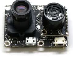
Figure 2.1 Flow rate sensor used in the project. Shown here with the included ultrasonic

distance sensor. . . 5

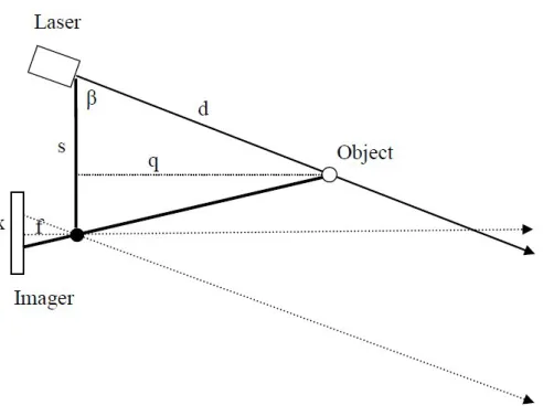
Figure 2.2 Visual representation of the geometry behind the distance sensing in the laser distance sensor (LDS) used. . . 11

Figure 2.3 An RPLidar laser distance sensor was used in the project. . . 11

Figure 2.4 RPLidar room scan example. It captures distances in all angles, taking a planar slice of the room. . . 12

Figure 2.5 Overview of Radio Control(RC) signal-flow. Ordinarily, RC signals originate at the remote, get transferred to the receiver over radio frequency and then are wired directly to the flight board. In this project, an RC Multiplexer(RC-Mux) is used to switch between sending the signals directly to the flight board, or passing them through the collision avoidance system. . . 13

Figure 2.6 Projecting the future path of the UAS based on current estimates of motion. . 14

Figure 2.7 Moving forwards towards a wall. As the UAS approaches the wall the disal-lowed stick position grows. At t=t2any forward inputs are instead overridden into backwards inputs. . . 17

Figure 2.8 Moving right towards an obstacle. The allowed right authority is progressively reduced until the pilot is only able to provide the correct inputs away from the wall. If the pilot doesn’t do so, the system overrides the pilot’s input by the computed necessary amount based on the Control calculations. . . 17

Figure 2.9 In special cases such as diagonal approaches, the disallowed area affects both the pitch and the roll portions of the piloting spectrum. . . 18

Figure 3.1 The assembled UAS showing the RPLidar as well as the BeagleBone-Black and all the sensor wiring to the PCB. . . 21

Figure 3.2 Underside of the UAS assembly showing the power distribution cabling, the battery, and the flow rate sensor. . . 21

Figure 3.3 The larger, final frame used for the Project. 750mm diagonally across, with 250mm diameter props. . . 22

Figure 3.4 Flowchart of the power distribution on the UAS. . . 23

Figure 3.5 Layout of the individual components on the PCB. . . 24

Figure 3.6 Software system overview. . . 25

Figure 3.7 Telemetry GUI developed for the project showing both the real-time graphs and the overhead map. . . 30

Figure 4.1 Example of cleaned up altitude estimation. Raw measurements are shown in blue, Kalman filtered estimate is shown in red. The estimate remains consis-tent even with multiple invalid readings in a short period of time, and while reversing the direction of motion . . . 34

(7)

Figure 4.3 Example of data exhibiting the scaling bug . . . 37 Figure 4.4 Data was collected at a significantly faster rate than previous ( as can be seen

by the range of the X-axis) in order to test whether speed was a factor in the accuracy or was causing bugs . . . 38 Figure 4.5 Graphs of altitude hold testing. . . 39 Figure 4.6 Screengrabs from the included video of testing. At this point the UAS is

head-ing towards the wall on the right at about 1m/s velocity. . . 40 Figure 4.7 As the UAS closes in on 1m from the wall (marked on the ground by a line of

tape) it rolls in order to move away from the wall. . . 40 Figure 4.8 While it lost some altitude in the process, the UAS sucessfully avoided crossing

the 1m line, as was the goal of the test. . . 40 Figure 4.9 The top plot shows distance from the obstacle. The green line is the minimum

distance for correction (2.5m). Only after the UAS crosses that line, will the corrections take place. We can see that even at speeds up to 2m/s the UAS always managed to recover before the 1m mark. The second plot shows the Roll values throughout the test. The green line is the corrected roll computed and applied by our control system, the blue line is the user input roll. From this plot it is clear to see that the corrections were all accomplished by the system. The only role of the pilot is to provide positive roll (right motion) in order to make the UAS drift towards the wall. Throughout the length of the test the pilot never aided the UAS in avoiding the obstacle. The third plot shows the X velocity throughout the test (X in this case is positive going right, and negative going left. This run was captured on video and can be found at

https:

//drive.google.com/open?id=0BylT1iNcfXLFZ3JrTWhYYVY4aFE

. . . . 41 Figure 4.10 These plots are from a similar test, with similar results. This run was also

(8)

CHAPTER

1 PREVIOUS RESEARCH

A review of previous researched was performed for the purposes of this project. It focused on both the use of specific technologies in the Unmanned Aerial Systems(UAS) field, technologies such as

Optical flow and Laser distance sensing, as well as work that integrated multiple types of sensors and

data into full fledged navigation solutions. Optical flow for odometry has been used in ground based robots in the past such as in[RDW12]and[SIY10]. For this project we looked at previous work for

odometry using optical flow in flying platforms. In[MKKGG15]More et al use a ordinary USB webcam

along with an ultrasonic distance sensor and an Intertial Measurement Unit(IMU), and implement an optical flow algorithm for motion estimation onboard a UAS. Readings from the distance sensor

and IMU are used together for angular compensation of the optical flow estimate. More recently the

group in[HMTP13]developed an all-in-one solution for optical flow estimation designed specifically for use in UAS applications. This camera handles all optical flow processing on-board and has

increased robustness to low-light environments. Angular compensation is accomplished much like

in[MKKGG15]using a combination of IMU and ultrasonic distance readings.

Laser distance sensors have long been used for SLAM and other environment sensing purposes,

but up until recent years have been far too heavy to be viable for UAS platforms. Recently research has been done using smaller lidars as in[CLDLCL14]for obstacle detection in UAS. The type of

(9)

CHAPTER 1. PREVIOUS RESEARCH

but maintains the level of coverage and accuracy. Due to its reduced cost and size it is extremely suitable for UAS applications.

There’s been quite a volume of research pertaining to autonomous indoor navigation of UAS,

as evidenced by the work in[SMK11],[FHHLMTP12],[WCPCL13]and[BHR09]. This is a different approach to collision avoidance than the one taken in this project. With autonomous navigation,

collisions are avoided by the path planning algorithm. This approach leads to never ending up in

a situation where the UAS has to actively take action to avoid an imminent collision. This type of research, however, has a lot in common with this project in the type of sensing that it requires. The

team in[CLDLCL14]built a UAS to navigate in a forest environment. This shares a lot of similarities

with our plan in that it uses a 2D laser scanner for obstacle detection, and an IMU combined with SLAM for motion estimation. The group in[SMK11]use SLAM along with data from an IMU to

create a sophisticated self location and mapping system. The system used loop closure to reduce the

error from SLAM as the UAS traverses the environment. Both in[WCPCL13]and[BHR09]location of the UAS is estimated using Kalman Filter fused data from SLAM, Optical flow and an IMU, while in [CLDLCL14]SLAM and IMU readings are used. The teams in[CLDLCL14],[SMK11]and[WCPCL13] used advanced motion capture and characterization systems to characterize the dynamics of their UAS, and determine the parameters of their respective controllers. This allowed them to develop a

model relating the controllable inputs pitch,roll,throttle,yaw to the motion of their platform. With this model they could then safely simulate most facets of the algorithm and tune off-line, before

testing on a live platform. The system in[WCPCL13]handles everything on-board and live, while

the system in[BHR09]handles most processing at a ground station, and has a 1-2 second delay for SLAM scan-matching which makes navigation slow. That system, however, was developed over 5

years ago and given current technology, the same processing could most likely be handled on-board

and closer to real-time.

Specific to collision avoidance there has been very little documented research from what I could

find. The group in[GMP15]and[FTRLGS14]use a very similar approach, ultrasonic sensors in

the cardinal directions, as well as up and down. In the case of[GMP15], proportional control was implemented, in the case of[FTRLGS14], the ultrasonic readings are used to implement

differen-tial control with fuzzy estimation of velocity from sequendifferen-tial distance measurements fused with

acceleration data from an IMU. Estimating velocity from scarce ultrasonic distance measurements has clear limitations. There’s no guarantee that the distance change is due to motion of the UAS,

rotation of the UAS, or motion in the environment. Using only 4 ultrasonic sensors leaves the UAS

susceptible to crashing when approaching objects diagonally, this fact, paired with the inability to get reliable estimates of velocity from simply ultrasonic sensors paired with an IMU, leaves a lot to

(10)

CHAPTER 1. PREVIOUS RESEARCH

Chinese company DJi is marketing a similar system. The DJi guidance. In addition to the ultra-sonics in the cardinal directions, this system improves on the reliability of the distance measurement

through estimating optical flow using 5 depth capable cameras. Said cameras also aid in the distance

measurements for collision avoidance.

This thesis project’s research lies somewhere in the intersection of autonomous navigation and

collision avoidance. Using the research into autonomous navigation, and the proven methods for

motion estimation and obstacle detection, this project’s UAS attempts to take all the knowledge of the environment that would be required for autonomous navigation, and uses it in service of aiding

(11)

CHAPTER

2 DESIGN

2.1 Estimating UAS Position and Velocity

Locating the UAS and determining its velocity will be accomplished with a combination of three systems. Optical Flow from a dedicated Optical Flow camera, SLAM using a 2D laser scanner, and

Dead Reckoning estimation based on readings from an IMU. These three different estimates will be fused using a Kalman filter into a unified, more reliable and robust estimate.

2.1.1 Optical Flow

Optic flow is the concept by which optical mice operate. It relies on taking snapshots of the

en-vironment around a moving object, in this case the ground beneath the UAS, and detecting the motion of that environment. The direction and magnitude of the motion of the UAS, can then be

estimated using the motion of the environment. In order to match points between snapshots, a

simple yet effective assumption is made. That pixel intensities stay constant from one snapshot to the next[FW06].

(12)

2.1. ESTIMATING UAS POSITION AND VELOCITY CHAPTER 2. DESIGN

Figure 2.1 Flow rate sensor used in the project. Shown here with the included ultrasonic distance sensor.

While this may not be true in all cases, it is enough to reliably match points in a majority of cases. One can then derive the gradient constraint equation[FW06]

ÏI(x~,t)·u~+It(x~,t) =0 (2.2)

whereu~is the optical flow. This equation can then be applied to multiple pixels in the image,

and under the assumption that neighbouring pixels share the same 2D velocity, the optical flow can be resolved using Least-Squares estimation[FW06].

The sensor chosen for the project was the PX4Flow sensor from 3DR. It does all the processing

on-board and as such simplifies the development significantly.

2.1.2 IMU Dead Reckoning

Dead reckoning navigation is the concept of self-location by estimating displacement, originating at

an initial unknown point, using measurements of velocity and acceleration. Using measurements of acceleration from an IMU, once can achieve a fairly reliable solution for dead reckoning navigation.

An IMU consists of a combination of Accelerometer, Magnetometer and Gyroscope. The

accelerom-eter measures acceleration. This acceleration vector, however, includes gravity. As such, in order to get a measurement of the linear acceleration of the IMU one must first remove the component of

the acceleration due to the force of gravity. In order to do this the orientation of the IMU must be

determined. Orientation estimation can be achieved in two ways. The first one of which is through trigonometry, using the acceleration information provided by the accelerometer, one can calculate

pitchandrollas

p i t c h=tan−1(_q Ax (A2x+A2_z

(13)

r o l l =tan−1(−Ax Az

) (2.4)

where the acceleration vectorA~= [A_x,A_y,A_z]. The second method requires use of the Gyroscope. Gyroscopes measure angular velocity. An estimate of absolute angle can be obtained by integrating

the angular velocity measurement with respect to time. Once the orientation is known, it can be

used to extract the linear acceleration from the absolute acceleration as shown below

Ac c e lLi n e a r=Ac c e lT o t a l−O r i e n t a t i o n·

0, 0,−g (2.5)

Estimates of velocity and displacement can then be calculated by integrating linear acceleration

with respect to time, once for velocity, twice for displacement. It is important to note that through

integration, errors accumulate linearly for velocity, and exponentially for displacement. This means that a small error in acceleration present throughout the measurement time, can lead to an

unac-ceptably large error in displacement estimation after a small amount of time. The state of current

sensor technology means that accurate dead reckoning estimation using only an IMU leads to large errors if used on its own for long periods of time. This is why our system aims to fuse dead reckoning

estimation with other sensor estimates using a Kalman filter. Similar solutions are used successfully in production systems ranging from GPS turn-by-turn navigation, and cruise missile navigation.

2.1.3 Data Fusion

Each method described previous suffers from different errors and failure states. On their own, they

might be sufficient to provide an estimate of pose and velocity of the UAS. Fusing the individual estimates using a Kalman filter, however, will produce a much more reliable estimate with greatly

reduced error. Kalman filters work by keeping track of an internal state x, that is related to a set of

measurementszby a state transition matrixA. This state transition matrix models the progression of the states over time. Future states are calculated by multiplying the current state estimate,

deter-mined using a combination of the latest measurement and the previous states, byAas shown by the

following equation

ˆ

xk=A xk−1 (2.6)

where ˆxk is the predicted state,Ais the state transition matrix and ˆxk−1is the previous state. In some systems one can also model a control inputu, that is related to the state by the control matrix B. In our case, since we’re dealing with a very complex nonlinear system, and ever evolving dynamics

(14)

properly implement a control input u within the scope of this project. In an ideal world, however, a properly modelled input matrix, relating pitch, roll, yaw, and throttle, to acceleration, velocity and

position, would aid greatly in the Kalman filter estimation. Including a control input would result in

the modified equation

ˆ

xk=A xk−1+B uk−1 (2.7)

whereBis the control matrix anduk−1is the control vector. The Kalman filter also keeps track of the internal state error covariancesPand calculates an internal termK, commonly referred to as

the Kalman Gain, that determines the weighting for the next state estimate. Intuitively, this means that while estimating the next state, the filter will either trust the model created based on past

measurements the most, or trust the latest measurement the most. The equations for the gain and

the predicted error covariance matrix are as follows:

ˆ

Pk=APk−1AT+Q (2.8)

Kk=PˆkHTS−1 (2.9)

Qis the estimated process error covariance. This is a constant value that attempts to capture the

level of noise inherent to the state estimation and is highly dependent on the model and its accuracy.

Ris the estimated measurement error covariance and is the equivalent ofQ, but with respect to the noise of the measurements. A proper value ofRcan be determined experimentally by collecting

sensor data.The next state is calculated using a combination of the predicted statexp, the latest measurement vectorz, the innovationy, which compares the predicted state to the measured state (effectively providing a measure of how accurate the previous state prediction was), and the Kalman

GainK, which includes all the filter’s errors: the process and measurement errors, that represent

how noisy the state predictions and the measurements are, respectively. The innovation covariance, which is a measure of how close the filter is predicting based on incoming measurements. And the

filter covariance, that keeps track of the errors of each state. The state and the covariance are then

estimated as shown below

y =zk−Hxˆk (2.10)

(15)

Pk= (I −KkH)Pˆk (2.12)

While in operation, the filter updates the states and covariances every time it receives a measure-ment. It then weighs the measurements and the internal state estimate according to their current

and overall noise levels, and constructs a smoother more accurate estimate of the states.

The matrices used in our system’s Kalman filter are outlined below. The state transition matrix models the relationship between the system’s measurements. Since we are collecting measurements

of acceleration, velocity and position, we can model their relationship and transitions with simple

kinematic equations

for a given time-stepdtthe acceleration, velocity and position of our UAS can be determined as

follows

pt =pt−1+vt−1∗d t +0.5∗at−1∗d t2 (2.13)

vt=vt−1+at−1∗d t (2.14)

a_t=a_t₋₁ (2.15)

In matrix form, and replicated for each of the three dimensions, these equations give us the

state transition matrixA

A=                 

1 d t 0.5d t2 0 0 0 0 0 0

0 1 d t 0 0 0 0 0 0

0 0 1 0 0 0 0 0 0

0 0 0 1 d t 0.5d t2 0 0 0

0 0 0 0 1 d t 0 0 0

0 0 0 0 0 1 0 0 0

0 0 0 0 0 0 1 d t 0.5d t2

0 0 0 0 0 0 0 1 d t

0 0 0 0 0 0 0 0 1

                 (2.16)

The measurement matrixH, converts the measurements into the states. In our case, the

mea-surements are the same as the states, so no conversion is needed, which would mean that if we had

(16)

2.2. OBSTACLE AVOIDANCE CHAPTER 2. DESIGN

Hvalues need to be set to 1. Our measurement matrixH is as follows, with a 1 at the z-position location, 1s at each of theVx andVy positions, and 1s at all of the accelerations.

H =                 

0 0 0 0 0 0 0 0 0

0 1 0 0 0 0 0 0 0

0 0 1 0 0 0 0 0 0

0 0 0 0 0 0 0 0 0

0 0 0 0 1 0 0 0 0

0 0 0 0 0 1 0 0 0

0 0 0 0 0 0 1 0 0

0 0 0 0 0 0 0 0 0

0 0 0 0 0 0 0 0 1

                 (2.17)

Finally, we need to determine values of process, and measurement noise. These will be

deter-mined experimentally and discussed in the implementation section.

2.2 Obstacle Avoidance

As stated previously, the goal of the system is to act as a safety net for an inexperienced pilot in an

effort to keep the UAS from being flown into obstacles. With that in mind the system has to allow the pilot full freedom to fly (unaffected) in open areas, but in (closed off areas) restrict the pilot’s

command authority to only the subset of inputs that will not lead to a collision. That is, given a

scenario where the pilot is providing a pitch forward input, and the UAS is approaching a wall in the forward direction, the system should increasingly restrict the pilot’s forward input, even going so

far as reversing it into a backwards output, to the extend required to keep the UAS from colliding

with the wall. In order to successfully accomplish this behaviour, the system must not only reliably detect objects as well as reliably estimate its own state (position and velocity). It also needs to be

able to capture and alter the pilot inputs promptly and accurately.

2.2.1 Obstacle Detection

Obstacle detection is of course key for any sort of collision avoidance system. There are a few

important considerations when choosing a sensor or this platform. Given the payload capacity of a

small UAS, the sensor needs to be lightweight. Low power would also be preferable given how little autonomy most small UAS’s already suffer from. Lastly, in order to be able to project this system

(17)

ranging units make use of time of flight calculations. These require extremely precise timing, which in turn require incredibly fast frequencies of operation, which drives up cost and size. A creative

laser ranging technique described in[KADFS08]opened the door for the benefits of laser ranging,

e.g.,360°field of view with degree accuracy from a single sensor, for low cost and size. The laser ranging technique described in[KADFS08]relies on triangulation. An image sensor is aligned with a

laser pointer, the laser reflects off an object in the distance and can be seen by the camera. As shown

in Fig. 2.2, by separating the laser pointer and the image sensor by a small distance and angling them towards each other by a minute angle, the sensor can detect shifts in the Z location(q) of the

reflection, as proportional shifts in the image axis(s). More specifically, from similar triangles, the

perpendicular distance to the object is

q= f s

x (2.18)

whereqis the distance to the detected object,f is the focal distance of the imager,sis the distance

between the imager and the laser, andxis the pixel distance between the ray parallel to the laser

and the ray from the detected object.

One limitation of this technique is that there is a hyperbolic relationship between image distance

( pixel displacement ) and object distance (perpendicular distance from sensor). This results in a

lessening of sensitivity at longer ranges, an illustrative example posed in the original paper specifies that if a 1 pixel image displacement corresponds to 10 mm distance displacement at 1 m, then it

corresponds to 40 mm at 2 m.

The RPLidar is the first consumer laser distance sensor (LDS) making use of this new concept, and is the sensor chosen for our platform due to its low cost and lightweight. The LDS outputs

distances up to 6 m away with 10 mm accuracy at 0.5°resolution. This is ideal for our application as

the given distance range and resolution will allow for reliable detection of obstacles in a vast majority of indoor flight scenarios, at an early enough time to have the system react to avoid a collision.

2.2.2 Capturing Pilot Intent

A majority of UAS are controlled using a combination of a remote(transmitter), a receiver and a flight control board. The remote generates multiple channels of pwm signals based on the position

of its joysticks. A typical setup would include 4 channels for the four main degrees freedom plus a

couple of additional auxiliary channels for additional optional modes. These signals are beamed to the receiver through a 2.4Ghz link to a receiver on the UAS, and then directly to the kk2 flight

board where they are converted to motor control signals. The flight board does the difficult task

(18)

Figure 2.2 Visual representation of the geometry behind the distance sensing in the laser distance sensor (LDS) used.

(19)

Figure 2.4 RPLidar room scan example. It captures distances in all angles, taking a planar slice of the room.

include a sophisticated auto-level system that makes the UAS easier to fly. In order to not have to

re-create the flight board, our system operates upstream from it, intercepting the signals coming from the receiver, and changing them, if necessary, before sending them back to the flight board. An

analogy would be that our system is acting as an extra pair of hands on the remote, correcting the

pilot’s inputs even when the pilot doesn’t realize they need to be corrected.

A RC Mux is used to allow the collision avoidance system to be turned on and off while testing.

This allows the pilot to switch to full manual control at any point, using a switch in the remote, in

the case that the collision avoidance system begins behaving erratically or experiences a crash. The signal flow is shown in Fig. 2.5

2.2.3 Altering Pilot Intent

The goal of the project is to combine robust velocity estimation, and reliable obstacle detection

in order to create a velocity based collision avoidance control system. Indoor navigation requires that the UAS fly close to walls, which could result in a collision. Without velocity estimation, an

"all-directions-are-dangerous" policy would have to be in place, which would generate problems in certain situations such as when going through doors, or flying close to walls. With velocity estimation,

one can project the future path of the UAS and only worry about avoiding collisions in that path.

(20)

REMOTE RECEIVER RC-MUX

Manual Control

FLIGHT BOARD COLLISION AVOIDANCE

Override

Select Channel

Figure 2.5 Overview of Radio Control(RC) signal-flow. Ordinarily, RC signals originate at the remote, get transferred to the receiver over radio frequency and then are wired directly to the flight board. In this project,

an RC Multiplexer(RC-Mux) is used to switch between sending the signals directly to the flight board, or passing them through the collision avoidance system.

that will make the UAS response more exact and reliable.

2.2.3.1 Projecting Craft Path

The UAS is only at risk of hitting static objects if they lie in the UAS’s future path. Assuming a reliable

estimate of velocity, one can project said path and only correct for obstacles lying in that path. The

advantage of this heuristic as opposed to considering objects in all directions is that the UAS can travel perilously close to obstacles, as long as it is not moving in the obstacles’ direction. This kind

of behavior is essential when navigating tight spaces, and allows for the system to support smaller

margins when it comes to distance from the UAS to obstacles. A disadvantage of this heuristic is that it does not react to moving obstacles if those lie outside of the UAS’s projected future path.

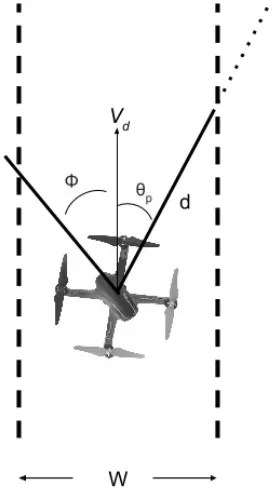
For a given velocity vector Vd and a given path-width W find all points (Lidar angle distance

pairs) that lie inside the projected W wide path. To accomplish this, we take every angle distance pair (σ+θp , d) provided by the Lidar scan, whereσis the angle of travel of the UAS andθp is the

angle of the detected point with respect to the lidar, as shown in Fig. 2.6, and calculate whether or

not, the point lies in the projected path. Points are in the path if

d< W/2

sinθp (2.19)

The algorithm to pick out the closest obstacle in the UASs path is explained in the pseudo-code

below.

(21)

Figure 2.6 Projecting the future path of the UAS based on current estimates of motion.

add d to pip // build a Points in Path list

}

pip = sort(pip) // Sort Points in Path ascending order

closestObstacle = median(pip, N) // Pick the median of the N lowest points

The first step is to determine whether the point detected is in the projected path. Once all the

points in the projected path are collected, they are sorted with the closest points being placed first. In order to mitigate false-alerts due to noise, the median of the N closest points is taken. This allows

for the system to be robust to N/2 spurious points, but it also means that an object must show up as at least N/2+1 points in order to be detected as an obstacle. W should be picked to be at least the width of the UAS. Larger W values allow for more robustness against noisy velocity estimation at the

cost of reacting to objects with which the UAS is at no danger of colliding with.

2.2.3.2 Calculating Necessary Corrections

Horizontal and Vertical control are handled independently. Given that the majority of the motion in which the UAS is likely to encounter obstacles is in the horizontal plane, the control system reduces

(22)

scenario results. Given this simplification, the system is susceptible to crashing if altitude is highly variable during flight and obstacles "appear" suddenly due to altitude variability, i.e. flying diagonally

upwards into a doorframe. In its current state the system is also susceptible to crashing into obstacles

above it. However, it would be trivial to extend the current system to allow for detection of obstacles above the UAS.

Horizontal control The necessary corrections to the pilot inputs are calculated based on the

difference between the minimum safe distance and the distance to the closest obstacle

e r r o r=M i n i m u mSa f e D i s t a n c e−D i s t a n c e C l o s e s t O b s t a c l e (2.20)

The corrections map directly to the four cardinal directions in which we can apply movement

outputs. As such the error must be rotated appropriately such that it matches those 4 directions.

The first step is to determine, which of the four quadrants the angle of the UAS motion lies in. The angle is calculated with trivial trigonometry as

a n g l e o f m o t i o n=tan−1Vx Vy

(2.21)

where Vx is the x component of the UAS velocity, and Vy is the y component of the UAS velocity. Determining the quadrant will tell us which of the 4 outputs (pitch+, pitch-, roll+, roll-) need to be

changed. i.e. if the angle is 32, it lies in the first quadrant, therefore the corrections that need to be applied are the outputs corresponding to that quadrant, and are pitch+and roll+. These are scaled

based on the angle as follows, assuming the angle from the example above

pitch+_error = error * sin(angle);

roll+_error = error * cos(angle);

pitch−_error = 0;

roll−_error = 0;

These errors are then multiplied by the proportional control gain K on-route to computing

a correction amount for each direction of travel. Additionally, a component of the correction is determined by velocity. The magnitude of the velocity, scaled by the derivative control gainKd, is added to the correction. In this scenario, the velocity acts as the derivative portion of the PD

controller.

// correction due to forward obstacles, to be applied negatively to pitch

correction[0] = pitch+_error * K + velocity_magnitude * KD;

(23)

correction[1] = roll+_error * K + velocity_magnitude * KD;

// correction due to back obstacles, to be applied positively to pitch

correction[2] = pitch−_error * K + velocity_magnitude * KD;

// correction due to left obstacles, to be applied positively to roll

correction[3] = roll−_error * K + velocity_magnitude * KD;

Vertical control Vertical control is only tasked with maintaining altitude. The error is therefore

the difference between the UAS altitude and the desired altitude.

e r r o r=D e s i r e d Al t i t u d e−C u r r e n t Al t i t u d e (2.22)

Since the Kalman Filter also provides an estimate of vertical velocity, it is used as the derivative

portion of a PD controller. Altitude in a UAS is determined by throttle, as such, these corrections are

applied to the throttle values.

Override - Limiting Pilot Authority The aim of the collision avoidance in this project, was to

avoid collision but by only acting when necessary, and incrementally. Many of the commercially available e-bumper solutions take a binary approach, where full control of the UAS is taken away

when dangerously close to an obstacle. The aim with this system was to operate just as effectively

at avoiding collisions, but to do so more seamlessly. The solution developed was an override, that takes the corrections computed by the control module, and determines the set of pilot inputs that

will result in a crash. It then does not allow the pilot to provide those inputs. In practice, say in the

case of moving towards a wall to the right of the UAS, this results in the pilot’s right motion authority being reduced, the closer they are to an obstacle on their right, to the point where their authority

will be limited to only left motion. The override scheme has the advantage of not being dependent

on how incorrect the pilot’s inputs are. It is only dependent on the distance from the obstacle, the velocity of the UAS and the gains of the control system. Another advantage is that in the case of

really close quarters flight, where there are obstacles in every direction that the UAS has to worry

about, the incremental nature of the override scheme will result in reduced command authority in the direction of the obstacles, even before a collision needs to be actively avoided. As an example,

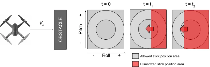
when navigating a long tight corridor, the pitch authority will remain unchanged, while the roll

authority will be limited proportional to how small the width of the corridor is. The figures below show different scenarios, along with the override scheme taking effect at limiting the area in which

(24)

Figure 2.7 Moving forwards towards a wall. As the UAS approaches the wall the disallowed stick position grows. At t=t2any forward inputs are instead overridden into backwards inputs.

Figure 2.8 Moving right towards an obstacle. The allowed right authority is progressively reduced until the pilot is only able to provide the correct inputs away from the wall. If the pilot doesn’t do so, the system

(25)

Figure 2.9 In special cases such as diagonal approaches, the disallowed area affects both the pitch and the roll portions of the piloting spectrum.

2.2.3.3 Air Brake

Unlike ground vehicles, UAS are highly susceptible to drift. Either due to external forces or due

to maintaining momentum from previous maneuvers, UAS can drift at high speeds and for large distances without any pilot input. This behavior is unacceptable when navigating in tight quarters,

and while ideally, obstacle avoidance would keep the UAS from hitting any walls while drifting

around, this is overall undesired behavior. A UAS that air-brakes, i.e., maintains x-y position when no pilot input is present, would prevent drift overshoot caused by obstacle avoidance corrections

and would also allow inexperienced pilots time to "breathe" without always having to worry about

maintaining UAS position by counteracting drift. The Air Brake system is an alternate control scheme that is only engaged when there is none/or negligible pilot input, and when the UAS is outside of the

minimum safe distance from obstacles. When engaged, the algorithm collects the current position p_b = [x_b,y_b], and then actively attempts to stay as close to it as possible. This is implemented through a PID controller in which the errors are the x and y distances from the brake pointpb

e r r o rx=xb−x (2.23)

e r r o r_y =y_b−y (2.24)

In addition to proportional control based on the distances, the x and y velocities are also being

(26)

e r r o rDx=v e l o c i t yx (2.25)

e r r o rDy =v e l o c i t yy (2.26)

This controller actively determines the pitch and roll outputs that would bring the UAS x and y

position back top_b, and its velocity to 0.

C o r r e c t i o nx=e r r o rx∗Kp+e r r o rDx∗Kd (2.27)

C o r r e c t i o ny =e r r o ry∗Kp+e r r o rDy ∗Kd (2.28)

2.2.3.4 Altitude Hold

Altitude hold might seem like an unintuitive choice for a collision avoidance package. But it actually contributes quite a bit, especially in the case where the UAS has a human pilot. Horizontal collision

avoidance will, if the velocities involved are large, induce a significant pitch/roll angle, which, given

the dynamics of the multi-rotor system, cause the lift vector to decrease in magnitude, and the UAS altitude to drop. An altitude hold system with a short enough reaction time would be able to

compensate for the loss of lift and maintain a constant altitude. Furthermore, altitude hold allows

the pilot have one less thing to worry about. The throttle would no longer be a property in need of active management by the pilot, and as such, increased attention could be focused on traversal.

The PX4Flow sensor includes a downward facing ultrasonic distance sensor, as part of its velocity

estimation solution. Internally it even compensates for errors due to pitch and roll angle. As such, our system can leverage those distance measurements, and include them in the Kalman Filter.

Using estimates of z-position and z-velocity, we can then construct a PID Controller where the

proportional error is the z-distance to the desired altitude, and the derivative error is the z-velocity.

e r r o rp=d e s i r e d Al t i t u d e−p o s i t i o nz (2.29)

(27)

CHAPTER

3 IMPLEMENTATION

3.1 Airframe

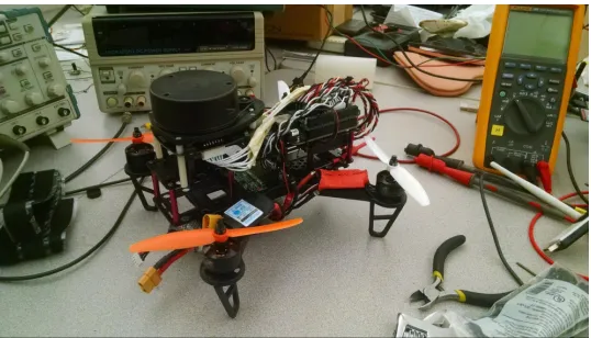
The UAS was custom built from COTS parts with a few considerations. The UAS had to be small enough to fit comfortably through a regular sized door. As such, a 250 sized frame was chosen, it

measures 250mm diagonally from motor shaft to motor shaft. Also, it had to have enough power to maintain maneuverability even with 1-2 extra pounds of hardware mounted on it. Proper motors,

props, and electronic speed controllers were chosen given this requirement. Lastly, it had to have

enough room to accommodate all the hardware mounting. Given the small size of the frame this was a bit of a close one, but all the hardware ended up fitting. The hardware was mounted using a

combination of screws, velcro and zip-ties. While it was important to make sure sensors like the

IMU and the Flow rate sensor didn’t vibrate in order to reduce noise in the data, the additional weight and development time that would be required to machine custom mounts was not available.

(28)

3.1. AIRFRAME CHAPTER 3. IMPLEMENTATION

Figure 3.1 The assembled UAS showing the RPLidar as well as the BeagleBone-Black and all the sensor wiring to the PCB.

(29)

3.1. AIRFRAME CHAPTER 3. IMPLEMENTATION

Figure 3.3 The larger, final frame used for the Project. 750mm diagonally across, with 250mm diameter props.

Frame Change The thought behind picking a small frame was to allow for navigating through

small spaces like doors. An essential feature of indoor environments. On the surface, the airframe has enough space for sensor mounting, and enough power to fly with the added weight. However,

some issues propped up once everything was mounted and the first test flights were conducted.

The craft was very unpredictable and it was clear from piloting that the auto-level system was working over-time just to keep everything stable. This meant that occasionally the craft would get

into an unstable state and odd things would occur, like sudden pitch or roll fluctuations, or the pilot

losing complete yaw authority while the craft enters a horizontal spin. Another issue, was that the craft took a lot of throttle to get off the ground, and when given 90-100% power, it would seemingly

lose power altogether and quickly lose altitude.

These symptoms all pointed to the airframe operating at the edge of its performance envelope. The cause of which was most likely a combination of two factors. The first was the use of a battery

that was too small, a 3S (11V) battery was used and an upgrade to a 4S(15V) battery would increase

thrust capacity, and therefore performance, by about 30-40% and would most likely help in fixing some of the flight performance issues. The second issue was the distribution of weight on the frame.

Due to the limited space, and due to requirements in the mounting of certain parts and sensors, (i.e.

the flight board needs to be mounted at the center of the frame, the Lidar needs an unobstructed 360 view, the optical flow sensor needs clear line of sight to the ground) the weight distribution

on the frame was far from ideal, with most of the weight being concentrated on the front of the airframe. There was no way to fix the second issue without switching to a larger frame.

The decision to switch to a larger frame was taken. Using a larger frame fixes the performance

(30)

3.2. HARDWARE CHAPTER 3. IMPLEMENTATION

more than enough thrust to perform with all the payload even with a 3S battery. The larger frame also means that all the sensors can be mounted centrally on the frame. Due to the higher thrust

and the better sensor placement, the flight performance of the frame with, and without the sensor

package is nearly indistinguishable.

Other advantages of the larger frame were found as testing progressed. Larger props lead to

much more efficient power consumption during flight, this means that the larger frame has a much

longer battery life, which is incredibly useful during testing, as it reduced the number of trips to the testing site, and as such speeds up progress. Also, the larger frame is much more sturdy and reliable.

During testing it took dozens of falls, some from free fall at up to 2 m. All of which caused no damage

to the hardware, and little to no damage to the frame. All of which would’ve most likely resulted in heavy damage to the smaller frame, and most likely the sensors as well, given how exposed they

were due to their mounting position.

Ideally, and eventually, a collision avoidance system like the one developed in this project would be mounted in a 250mm sized or similar frame, but for prototyping and testing, it seems obvious

now, looking back, that a larger frame is be the best option for development.

3.2 Hardware

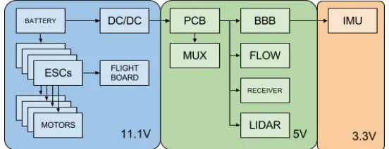
A PCB was custom designed to serve as power distribution and sensor interfacing. A DC/DC step

down converter brings power from the battery, stepping down to 5V, to the PCB. The 5V are then routed to power both the BeagleBone Black and the sensors as shown in the diagram below.

Figure 3.4 Flowchart of the power distribution on the UAS.

The PCB was built as a BeagleBone Black cape and has connectors for the Flow Rate sensor, the

(31)

3.3. SOFTWARE CHAPTER 3. IMPLEMENTATION

(which also can be mounted right on the PCB). The direct mounting of the Multiplexer greatly reduces the amount of cabling required to wire the system to the receiver and the flight board.

Figure 3.5 Layout of the individual components on the PCB.

3.3 Software

The software consists of a single multithreaded C++program, instantiating a multitude of classes

that each have their own independent task, and run on their independent threads. The main program

(32)

3.3. SOFTWARE CHAPTER 3. IMPLEMENTATION Main Software Corrected PWM Wi-Fi PX4Flow BNO055 RPLidar BNO055 Driver PX4Flow Driver RPLidar Driver

I2C UART UART

KalmanFilter Acceleration Control Velocity Velocity Data Packet Telemetry Telemetry GUI PWM PWM Corrected PWM PWM Flight Board

Remote Drone Motors

[Distances, Angles]

Figure 3.6 Software system overview.

The sensor objects each collect their respective sensor’s data. That data is transmitted to the

correct modules by the main program, for example, in the case of the Kalman filter, the main program fetches the measurements of acceleration, velocity and position, from the different sensor objects

and provides them to the Kalman Filter object. The Control object receives pilot intentions, in the

form of PWM values from the PWM object, along with Velocity estimates from the Kalman Filter, and measurements of Distance from the Lidar object. Using this data the Control object computes the

necessary corrections to be made to the PWM values. These are then fed back to the PWM object by

the main program. The PWM object then applies these corrections to the PWM values and readies them to be sent to the Flight Board.

3.3.1 BNO055

The BNO055 object handles the communication with the BNO055 IMU. There is an existing arduino

(33)

not an Arduino platform. The object was then wrapped in another class to make usage in our system more streamlined

// create the imu object

IMU imu = IMU();

// connect to the IMU

imu.init();

// update acceleration and orientation based on latest IMU reading

imu.update();

// return acceleration

float[3] acceleration;

acceleration = imu.getAcceleration();

Orientation Sensor Calibration The orientation sensor used, Bosch’s BNO055, does automatic calibration upon reset. Unfortunately this requires a set of maneuvers ranging from doing figure 8s

in the air, to calibrate the magnetometer, to slowly transitioning between and holding 6 specific

positions, to calibrate the accelerometer. Given that the sensor is mounted on a large frame, and given that the battery has to be swapped at most every 20 or so minutes during use, one would

obviously prefer not to have to execute this calibration "routine" after every boot-up. On the other

hand, having un-calibrated sensors is also unacceptable, given that that’s an easily squelched source of error in the system, that affects both the Kalman filter states, and the orientation estimation. As

such, effort was put into researching how to save and load calibration data at start-up. As described

in the data-sheet the calibration registers are registers 0x55 through 0x6A. By placing the sensor in configuration mode one can read the registers after calibration. Once those values are saved, it is

simply a matter of writing those values to the correct registers after boot-up.

3.3.2 Flow Rate Sensor - PX4Flow

Communication to the PX4Flow was made over UART at 115200 BAUD. The driver was written from

scratch. It handles the UART link creation as well as the message parsing. The PX4Flow transmits

data in the form of MAVLink messages. These start with a common start byte, 0xFE, that serves to signal the start of the message header. The header is standard and can then be parsed. The

information in the header serves to determine how to parse the incoming message. It contains

(34)

// create the PX4Flow object

PX4Flow flow = PX4Flow();

// establish the UART connection

flow.init();

// collect another set of flow rate and ground distance readings

flow.update();

// return flow₋rate in the X axis

float flow_x;

flow_x = flow.getFlowX();

3.3.3 Laser Distance Sensor - RPLidar

The goal of the Lidar driver is to handle all sensor specific interfacing, and make as easy as possible

for the main program to get the latest distance readings. The provided RPLidar sdk was used as a base. The sdk handles the communication with the Lidar over UART at 115200 Baud. A C++class was created to abstract away the creation of the Lidar object, and the updating of the lidar readings.

Said object also keeps track of the distances as an internal 360 member integer array. Example usage

of the class is shown below.

// create the lidar object

RPLidar lidar = RPLidar();

// connect to the lidar

lidar.init();

// update distances based on latest lidar reading

lidar.update();

// return distances

int[360] distances;

distances = lidar.getDistances();

3.3.4 Kalman Filter

For including the Kalman filter, two classes were created. One to serve as a generic all-purpose

(35)

filter variables etc... Another class was then created to instantiate this first class and provide it with the matrices specific to our UAS scenario. It initializes the generic Kalman Filter with the correct

state transition matrix, correct measurement and process errors, as well as correct observation

matrix. One can then simply provide new measurement vectors to this class and it handles all the computations internally. An example of usage is shown below.

// create the Drone Kalman Filter object

DroneKF kf = DroneKF();

// initialize the filter object: give it an initial state, create the

internal KF filter etc...

kf.init();

// set measurement to be used in the next filter step

kf.setMeasurement(float[3] position, float[3] velocity, float[3] acceleration

);

// step the filter forward

kf.update();

// get the filter state vector

float[9] state;

state = kf.getState();

3.3.5 Control

The goal of the control module is to take the UAS velocity and distances to obstacles as inputs, and

compute the amount of correction that needs to be applied to the pilot inputs. In order to do this,

the software projects the path of the UAS based on its current velocity, and finds the closest obstacle in that path. The distance to that obstacle is then used to determine the error in the PD controller.

The control module handles both horizontal and vertical control independently.

// create the Control object

Control control = Control();

// provide the control object with the latest distance measurements

Control.setDistances(lidar.getDistances());

// provide the control object with the latest velocity estimate

Control.setVelocity(kf.getVelocity());

(36)

Control.setGroundDistance(kf.getPosition()[2]);

// update the correction values based on the latest measurements

Control.update();

3.3.6 Pulse Width Modulation(PWM)

The PWM module is in charge of capturing and altering pilot intent, based on the corrections

calculated by the Control module. This is achieved by two separate programs working in tandem. The measuring and generating of the PWM is handled by an assembly program running on one of

the Programmable Real Time Units in the Beaglebone Black. A real time controller is required since

the Linux Kernel running on the Beaglebone is not hard real time, and as such the measurements and generation of the PWM signals, are not guaranteed to be accurate at all times. The software

running on the PRU measures the pulse-width of the incoming PWM signals, and writes it to shared

memory for the main C program to use. It then reads back the modified pulse-width information from shared memory and generates said pulses. The modifying of the PWM signals based on the

Control outputs is handled by the PWM class, which is instantiated in the main C++program. This

class not only handles the reading and writing of PWM duty cycles to shared memory, but it also calculates the corrected PWM values based on the corrections computed by the control module.

Example usage is shown below.

// create the pwm object

PWM pwm = PWM();

// initialize the PRU and start running the assembly program

pwm.init();

// read write latest PWM values to shared memory

pwm.update();

// override pilot inputs based the outputs of the control module

pwm.override(corrections, verticalCorrections);

3.3.7 Telemetry

Monitoring the state of the UAS and its sensor readings in real time is essential for both successful

(37)

a Wi-Fi socket, and a java based GUI that receives the data and displays it in a data-type appropriate way ( an overhead map based on the lidar distances, stick position of the controller based on PWM

signals, graphs based on raw and filtered sensor data, etc...) this GUI is shown below.

Figure 3.7 Telemetry GUI developed for the project showing both the real-time graphs and the overhead map.

The GUI includes real-time graphing of the data being collected(1). The raw data is shown

in blue, the kalman filtered data is shown in red. The code is built so one can very easily change what data gets shown on the graphs for diagnostic. The 360 distance points from the lidar are used

to project a 2D overhead map of the environment(2). Also included, are vectors representing the

magnitude and direction of the acceleration, shown in red, and velocity, in yellow, of the drone(4), as well as highlighting of the projected path (the red portion of the lidar map at (3)) and the closest

obstacle, the pink line projected from the UAS onto the projected path at (4).Additionally, the panel

also includes RC remote inputs as well as control corrections(5).

The telemetry system also saves all the data to a .csv file and has the ability to play it back (6).

All while allowing the user to play, stop move frame by frame forwards and backwards, as well as

(38)

comb through and examine specific scenarios to determine what went wrong.

The Telemetry system was essential for debugging all the parts of the UASs software. It is also

invaluable while test flying, as it allows us to make dry runs while just looking at the data and make

sure the system is attempting to do the correct thing, before actually flipping the switch to turn the Control system on.

Example usage of the Telemetry class is shown below.

// create the telemetry object

Telemetry telemetry = Telemetry();

// make the socket connection to the Host Telemetry program

telemetry.init();

// create telemetry message

telemetry.packMessage(distances,rcSignals,corrections, etc...);

// send latest telemetry message

telemetry.send();

3.3.8 Configuration File

During the initial phase of testing, most of the constants used to tune the control algorithms were

kept in a header file and defined at compile time. This meant that while tuning the controller gains,

every time a gain needed to be changed, the entirety of the control software had to be rebuilt. At this point the software took about 1 minute to build. As such, in order to speed up and ease the testing

process, a solution was implemented that defined these constants at run-time, by reading them

from a configuration file. A header file, Params.h, outlines a shared data structure containing all the software constants. A C++file, Params.cpp populates the shared data structure at run-time by

(39)

CHAPTER

4 TESTING

4.1 Testing Issues

4.1.1 Reliability

Reliability was an issue during testing. Poor reliability came in the form of unhandled software

exceptions that cropped up occassionally. Time and effort was put into removing these exceptions when they occurred during project development, but most of the focus had to be set squarely

on project development tasks instead. Plenty of crashes or near misses were caused due to the

software crashes due to exceptions ocurring. It was noted that exceptions and crashes most often occurred at moments of high UAS acceleration, but are other times unrelated to physical forces

being experienced by the system. As a pilot it took a second or so to realize the system was "stuck"

at the last received command, and react in time by switching to manual control. If this happened in "open air" it was no problem but at times it happened right when approaching a wall. Three props

(40)

4.1. TESTING ISSUES CHAPTER 4. TESTING

4.1.2 Testing Alone

An unexpected difficulty of testing in this project was the fact that the pilot had to both be pilot

and real-time data analyst. While the Telemetry system was able to log data, looking at logs pales in

comparison to being able to see the UAS behaviour and the returned sensor data in real-time. Many testing scenarios were made much harder by having to either try to keep an eye on both the data

and not crash the UAS, or having to go back through logs after the flight trying to piece together

what part of the flight the data was from. Testing help was arranged towards the end of the project. But having another person helping the pilot during testing would’ve been beneficial to the progress

of the project.

4.1.3 Altitude Hold testing

Data Quality Altitude hold relies on the ultrasonic sensor to provide accurate measurements

of the UAS distance to the ground below. The more unreliable these measurements are, the more

unstable the control will be. If these measurements are too unstable, the control algorithm becomes unreliable. As such, during testing, the initial focus was in quantifying the performance of the

ultrasonic sensor, and taking the necessary steps to getting a solid estimate of both ground distance,

and Z-velocity, as they would be the ingredients to developing a quality altitude hold control. Ultrasonic sensor performance is fairly sensitive to surface absorption properties. As such, the

initial plan to test over grass was quickly scrapped due to the ultrasonic sensor having a 30-40%

invalid reading rate on that surface. Over pavement the ultrasonic sensor readings were solid, but during testing a couple issues were found. The first was that occasionally the sensor would get an

invalid reading, that would show up as a negative number. If unhandled, this reading would cause

large spikes in the velocity estimation, and in turn large spikes in the control response. Another issue was that at distances higher than 3 meters, the ultrasonic sensor returned only invalid values.

In order to fix the above issues a couple of simple tweaks were made to the software. The first of which worked by leveraging the robust nature of the Kalman Filter. If the reading was negative (i.e.

invalid), the measurement was not fed to the Kalman filter. This was accomplished by dynamically

changing the Measurement Vector H, based on the validity of the ultrasonic reading. That way, the invalid reading doesn’t have a negative impact on the estimation. This worked for the occasional

invalid readings, however, for the case of constant invalid readings above 3m, the Kalman filter

estimation quickly broke down and relying on only past prediction and accelerometer readings values alone, accumulated a large error. This was fixed by setting a measurement ceiling at 3m as

described in the following piece of pseudo-code.

(41)

4.1. TESTING ISSUES CHAPTER 4. TESTING

currentDistance = 3000

These two changes in the software lead to robust estimation of both altitude and Z-velocity as

shown in Fig. 4.1

Figure 4.1 Example of cleaned up altitude estimation. Raw measurements are shown in blue, Kalman filtered estimate is shown in red. The estimate remains consistent even with multiple invalid readings in a short

period of time, and while reversing the direction of motion

Control Schemes Several control schemes were attempted for vertical control. Initially, and

in the spirit of only correcting the pilot if they were in danger of crashing the UAS, the system’s aim was to only correct throttle if the UAS was below a certain safe altitude. This however, meant

that the system needed to be robust to both slow descents into that dangerous altitude, as well

as fast freefalls, and by only acting after the UAS was already in a dangerous altitude, the system had to be incredibly agressive and have a very large margin to the ground. Also, due to the system

only "turning on" after a specific set point, and "turning off" above it, having a stable return to

the setpoint was unachievable, as there was no way to control the descent portion of the cycle. An attempt was made to mitigate this by allowing the derivative control to act at a larger distance from

the ground. This allowed the system to begin slowing down the descent of the UAS before it actually

reached the set point, and allowed any overshooting above the setpoint to be mitigated somewhat. This solution ended up being abandoned in favor of a true altitude hold.

In altitude hold, the system attempts to maintain the altitude at a variable set-point, controlled

by the throttle signal from the remote. This has the advantage of allowing the system to control both the ascent and the descent of the UAS. Unlike in the one-directional control schemes described

above, where the control system "releases" the craft once it’s above the setpoint, in altitude hold the

control system always is aware and correcting the craft’s behavior. This leads to a much more stable and controllable response. It is still a challenging problem due to gravity. The ascent response and

descend response need to be scaled to account for gravity, otherwise the system will be unstable

(42)

4.2. TESTING RESULTS CHAPTER 4. TESTING

are scaled down by this factor if the movement being induced is downward, and unchanged if the movement being induced is upward.

4.2 Testing Results

4.2.1 Self location

The aim of this test is to quantify the reliability of the position estimation of the system, this will

serve to determine the quality of the velocity estimation. While position estimation is itself not relevant for the performance of the collision avoidance system, the better the position estimation,

the better the velocity estimation. Accurate velocity estimation is essential since it is being used in

the path projection for obstacle detection, as well as the derivative term of the PD controller for horizontal collision avoidance.

With the absence of a motion capture system the testing was done by hand, by measuring a path

on the floor, and carefully moving the drone by hand along said path, at an altitude of roughly 1m. This means that there will be an error in the ground truth of about+/-50 mm due to human error.

During these tests the orientation of the UAS was kept as close to constant as possible. This

is to eliminate any errors in position estimation due to errors in the Yaw values. This means that the following 2D location graphs are relative to the UAS’s frame, which in the specific case of this

test, was made to be as close as possible to the World frame. The reason this isn’t an issue is that for

collision avoidance we’re only concerned with the velocity of the UAS relative to the obstacles its detecting. The obstacles are also being detected in the UAS’s frame, therefore there is no need to

"map" the UAS velocities to the world frame.

Results During testing an interesting, and yet undiagnosed, problem was discovered. The position estimation seems to be accurate, but scaled down. That in itself wouldn’t be a problem, if

the scale was consistent. It is not. While across the majority of the runs performed the scale of the resulting position estimates is 60% smaller than ground truth, occasional runs provided maps that

are seemingly correct (i.e. the traced path edges’ relative size matches, the path starts and ends at

the same location as expected), but scaled down to smaller than 60%.

Multiple tests were made to attempt to diagnose this issue. Height from the ground was tested,

since the focal length of the flow rate camera can have a small effect on the estimation, it was thought

that perhaps different runs, taken at different heights, would have different estimates of velocity.This was found to not be the case. Thankfully so, since if there was a significant difference in the velocity

(43)

possible culprit was the speed at which the path was run. Perhaps the camera has trouble picking up slower speeds. The path was run at different speeds in order to test this hypothesis, that also

didn’t prove to be the issue, the same problem kept propping up.

The graphs shown below are scaled by a factor of 1.6 due issue explained above. While multiple runs were made, only two graphs are shown below, to illustrate a graph with, and without the scaling

bug. These are illustrative of the "quality" of the other data collected. Roughly 1 in 5 collections

suffered from the scaling bug.

(44)

(45)

Figure 4.4 Data was collected at a significantly faster rate than previous ( as can be seen by the range of the X-axis) in order to test whether speed was a factor in the accuracy or was causing bugs

Looking past the scaling problem, the estimation is fairly consistent and somewhat reliable.

Errors of up to 300mm are found in most of the runs, but they seem to only occur at specific points in the path, where in the majority of the duration of the path the tracking is within+/- 100mm of

the truth. A possible cause of this is the orientation of the UAS not being kept quite as constant as

would be ideal, this would lead to errors in the velocity estimate, given that orientation isn’t being taken into account in this experiment.

4.2.2 Altitude Hold

The purpose of this test is to quantify the quality of the altitude hold. The factors being looked at are steady state error, i.e. how much the UAS drifts from the target altitude, and rise time, i.e. how long

it takes the UAS to reach the target altitude, both from below, and from above said altitude. While

altitude hold isn’t in itself essential for horizontal collision avoidance, it is important for vertical collision avoidance. Furthermore, horizontal avoidance might induce extreme pitch or roll angles

on the UAS, which will cause it to lose altitude, due to the thrust vector not being focused upwards,