Classical E&M Model for Nonlinear Optics - Applications to the Generation of Harmonic and Terahertz

(1)

Abstract

HAIJIANG PENG. Classical E&M Model for Nonlinear Optics ⎯ Applications to the Generation of Harmonic and Terahertz Radiation (Under the direction of Professor

David E Aspnes).

Nonlinear optical techniques have become very useful diagnostic methods for

surface and interface properties of materials and for developing new materials. However,

it is still very difficulty to interpret nonlinear optical data. Here, I continued to develop

the simplified bond hyperpolarizability model (SBHM). I extended the theory to describe

the bulk-forbidden second harmonic generation (SHG), bulk third harmonic generation

(THG), and fourth harmonic generation (FHG). I clarified the relative importance of

bulk-forbidden contribution and surface dipole contribution to SHG. I showed the

transverse-bond-direction motion was necessary to correctly describe THG data. And I

presented a way to evaluate the surface roughness effects on FHG.

In addition, from the principle of SBHM, I developed a simple model to interpret the

origin of terahertz radiation from semiconductor surfaces trigged by ultrashort laser pulse.

I unified the mechanisms of terahertz generation ⎯ difference frequency mixing and

current surge mechanism at the field level.

Finally, I showed spectroscopic SHG could give us more information than single

(2)

Classical E&M Model for Nonlinear Optics —

Applications to the Generation of Harmonic and Terahertz

Radiation

By

Haijiang Peng

A dissertation submitted to the Graduate Faculty of North Carolina State University

in partial fulfillment of the requirements for the Degree of Doctor of Philosophy

PHYSICS

Raleigh

2005

APPROVED BY:

Dr. Christopher Roland Dr. Hans Hallen

(3)

Dedication

To my grandmother Juyun Liu, grandfather Dongsheng Peng, my parents Funan

Peng and Meixiu Chen, my stepmother Shengchun Liu, and my girl friend Shuwei Wu

for their love.

(4)

Biography

Haijiang Peng was born in a small village in XiangTan County, XiangTan, Hunan, P.

R. China to Funan Peng and Meixiu Chen. His mother, Meixiu Chen, died a few hours

after his birth. He grew up with his grandparents until he was 10 years old. He then

stayed with his father and stepmother, continuing in elementary school in Changsha.

After completing the 9th grade, he passed the entrance examination for a special class, in which the students are trained specifically for attending the competition of

Olympic-Physics competition for middle-school students. Unfortunately, his first try in physics

was unsuccessful. He did not do as well as expected in the contest. However, he did not

lose confidence. He continued his goal of physics in the Department of Physics, Jilin

University, after his graduation from high school. In Jilin Unversity he was really

attracted by the world of physics and felt the power of physics. He started his research

under Prof. Chengxiang Zhang in solid state physics. After he obtained his bachelor

degree, he went to the Department of Physics, National University of Singapore. There

he worked on the growth of cobalt silicide for 0.18µm CMOS technology, which is

supported by the largest chip manufacturing company, Chartered Semiconductor

Manufacture Ltd. In this project, he published his first scientific referred-journal paper on

solid-state electronics, “Effects of First Rapid Thermal Annealing Temperature on Co

Silicide Formation”. Two years later, he went to Department of Physics, North Carolina

State University, to pursue his PhD degree under the direction of Prof. David E. Aspnes.

He and Dr. Aspnes worked together very well, publishing 5 referred journal papers.

(5)

Acknowledgements

Here, I would like to thank many people for their help and encouragement. Without

them, it would have been impossible to finish this project. First of all, I appreciate very

much my advisor, David E. Aspnes. His attitude toward science, his keen insight into

problems, his solid background on all aspects of physics, and his kindness are always my

good example and my motivation to be a professor. I also thank Committee members

Prof. Hans Hallen, Prof. Christopher Roland, and Prof. Robert M. Kolbas for their time

and consideration.

I must say that our group is very nice. Jon–K. Hansen, a visiting scientist from

Norway, helped me significantly at the beginning. I have very happy memories of our

discussions during lunch time. I would also like to acknowledge other group members,

Ji-Fu Wang, Muharrem Asar, Klaus Flock, Sungjin Kim, Nicholas Stoute, Eric Adles, Inkyo

Kim, and Xiang Liu. I will remember them always.

(6)

List of Tables

(9)

List of Figures

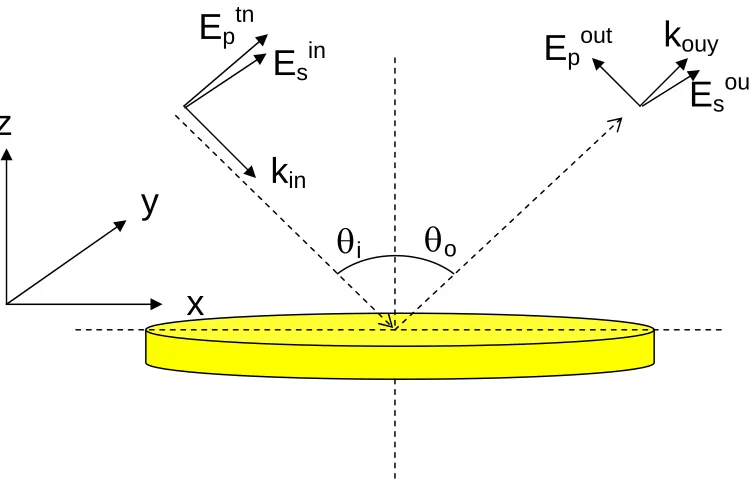
Figure 3.1 Experimental configuration for harmonic-generation measurements………..43

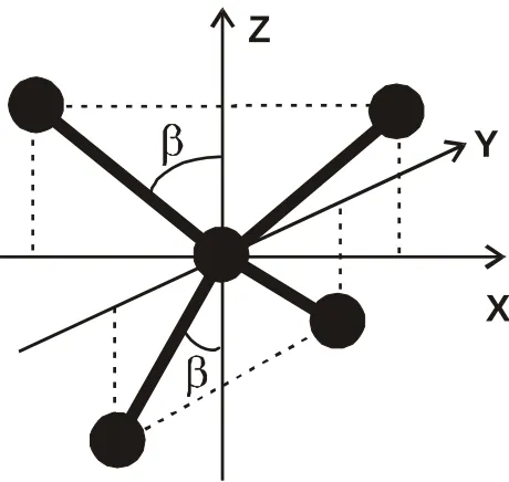
Figure 3.2 Bond-vector diagram………...44

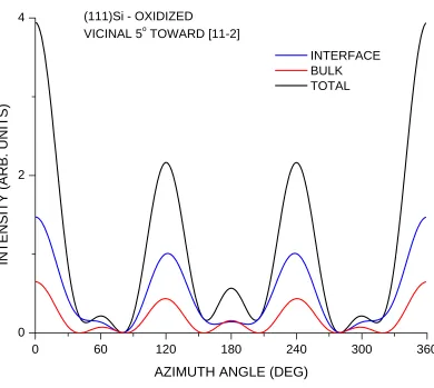
Figure 3.3 Anisotropy of SHG for vicinal Si 5° off (111) toward [11-2]………..45

Figure 3.4 Different contributions to the pp data of Fig. 3.2………46

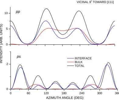
Figure 3.5 Anisotropy of SHG for vicinal Si 9° off (001) toward [111]………...…47

Figure 3.6 Different contributions to the data of Fig. 3.4……….48

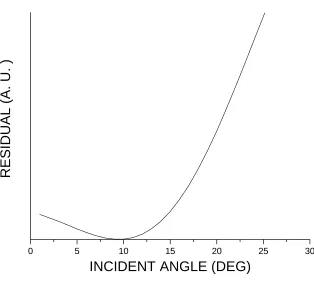
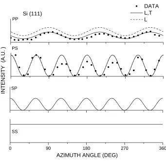
Figure 4.1 Azimuthal dependences of THG signals for vicinal Si (111) offcut 5° toward ] 2 11 [ . Points: data from Ref. 14. Lines: SHBM with longitudinal and transverse components both included (solid) and longitudinal component alone (dashed)…69 Figure 4.2 Best-fit residual as a function of angle of incidence qi………...70

Figure 4.3 As Fig. 4.1, but for on-axis Si(111). The data are from Ref. 20…………...71

Figure 4.4 As Fig. 4.1, but for Si (001). The data are from Ref. 20……..………72

Figure 4.5 As Fig. 4.1, but for Si (001). The data are from Ref. 14……..………73

Figure 5.1 Normalized FHG anisotropies for the (001)Si-SiO2 interface for the polarization combinations pp, ps, sp, and ss, as reported in Ref. 2. The solid curves are the results of the SBHM calculations………...86

Figure 5.2 Normalized FHG anisotropies of (001)Si immediately following exposure of the sample to a buffered oxide etch for durations of 0 (top), 10, 20, 30, and 60 min (bottom). The solid curves are the result of SBHM calculations taking into account interface roughening………..………..87

Figure 5.3 Normalized FHG anisotropies for the (001) Si-SiO2 interface for the polarization combinations pp and sp. The solid curves are the result of SBHM including interface roughness………88

Figure 6.1 pp- and ps- polarized FIR intensity for (001)InP. Data are from Ref.1…....101

Figure 6.2 Frequency dependence of the bond-charge contribution to the THz intensity. ……….102

Figure 7.1 SHG experimental configuration...……….106

Figure 7.2 Azimuthal-dependent data at difference wavelengths for samples with oxide-nitrided and oxide-oxidized layers with and without RTA on Si (111) surfaces tilted 5º towards (-1 -1 2)………..………...…………....107

Figure 7.3 Comparison of hyperpolarizabilities for samples with and without RTA: a, up bond; b, step bond; and c, back bonds……….………..108

(10)

Chapter I. Introduction

Optical probes have unique advantages that become more desirable when higher

spatial and temporal resolutions are required. Material damage and the buildup of

contamination layers associated with charged-particle exposure do not occur; no special

ambient conditions such as ultrahigh vacuum are needed; charging effects in insulators

are avoided; long penetration depths allow access to solid-solid and other buried

interfaces; and real-time, in-situ monitoring of film growth is possible [1-4]. These

advantages are important when exploring new materials, especially in the

nanotechnology era, and in applications to biology, where vacuum environments are not

relevant. However, optical techniques also have disadvantages when used for surface and

interface analysis. Signals are generally weak because of the weak interaction between

photons and matter [5], and data are often difficult to interpret [5]. For example, in

linear-optical measurements more than 90% of the reflection is due to the bulk, so the

signals from the interface/surface are relatively small and hence difficult to analyze.

We can classify optical techniques into two groups: linear and nonlinear. Linear

optical techniques involve the linear susceptibility, χ1, which is a second-rank tensor, and include laser light scattering (LLS), spectroscopic ellipsometry (SE), spectroscopic

polarimetry (SP), reflection-difference (-anisotropy) spectroscopy (RDS/RAS), surface

photoabsorption (SPA), photoluminescence (PL), etc. Nonlinear optical (NLO)

techniques such as second- (SHG), third- (THG), and fourth- (FHG) harmonic generation,

involve higher-order susceptibilities such as χ2, χ3, and χ4, which are third-, fourth-, and

fifth-rank tensors, respectively. Other NLO possibilities include optical sum-frequency

(11)

involved, NLO probes exhibit richer selection rules than linear-optic probes [6], so NLO

methods are potentially more powerful than linear-optic approaches as diagnostic tools.

Furthermore, because the symmetries of surfaces and interfaces are generally lower than

those of the bulk, some NLO approaches can be considered as only surface/interface

diagnostic techniques. For example, both SHG and FHG are dipole-forbidden in the bulk

of centrosymmetric crystals such as silicon [7-10], so if we ignore higher-order

contributions, either of these probes will return information only about Si surfaces and

interfaces.

Following the golden days of theoretical research in the 1960s and 1970s, interest in

NLO declined as a result of small signal strengths and the difficulties of interpreting data.

However, the development of the femtosecond (fs) laser changed the experimental

situation. By reducing pulse durations to the fs range, peak fields could be increased

substantially without violating the usual limit to signal strength, the average power

applied to a sample. The result for SHG was an increase in signal strength by 3 to 4

orders of magnitude. As a consequence, NLO has re-emerged as a viable experimental

approach for studying bulk material, thin films, interfaces, and surfaces.

However, until recently, the difficulties in interpreting NLO data remained. As we

noted, optical data are already difficult to interpret, and the situation for NLO is even

worse. One standard approach is the macroscopic tensor-coefficient representation. Its

basis is the relation between polarization and external field [11]. The approach takes

advantage of the known symmetry of a crystal. One first uses rotation to project the

applied field into the crystal frame, where the polarization is calculated. The polarization

(12)

expressions are used to obtain the observed harmonic fields. Another method is the

Green-function approach, where the NLO problem is solved using the classical E&M

Green-function formalism in terms of s- and p- polarized vector waves. This leads to

generated fields written as functions of the Fresnel coefficients of the interfaces [12].

The polarizable bond model calculates SHG in terms of the energy resonances associated

with the linear response [13], and in fact picks up only part of the total response, the

quadrupole contribution. Other methods such as quantum-mechanical evaluation of

polarizabilities from band structure, and simple listings of Fourier coefficients of

intensity anisotropies observed as the sample is rotated during exposure to a fixed

wavelength, are also used in some applications.

Unfortunately, none of the previous formalisms were simple enough to lead to

closed-form expressions or to provide useful or complete physical insight about the

origins of NLO signals on the atomic scale. These shortcomings were eliminated with

the development of the simplified bond-hyperpolarizability model (SBHM) of Powell et

al [14]. These workers introduced what they termed the SBHM to assist the analysis of

their SHG data obtained on Si-insulator interfaces [14, 15]. They showed that observed

SHG anisotropies could be described in terms of a hyperpolarizability associated with

each of 3 types of interface bonds as opposed to the 11 Fourier or 14 tensor characteristic

coefficients of previous work. Moreover, they showed that the 3 hyperpolarizabilities

determined from the observed intensity anisotropy of the pp polarization combination

could be used to predict the observed anisotropies for the ps, sp, and ss combinations.

Finally, they obtained analytic descriptions of these anisotropies in terms of these

(13)

SHG data, but also allowed them to be understood in terms of parameters that had direct

physical meaning on the atomic scale.

However, the question remains as to how general the SBHM really is. Powell et al.

did not address a number of NLO phenomena also of interest: FHG from Si-dielectric

interfaces, higher-order bulk contributions to SHG in centrosymmetric crystals, THG

from bulk Si, or the generation of terahertz (THz) radiation from semiconductor surfaces

and interfaces. Owing to the wide wavelength range involved and the relatively weak

signals associated with a high-order nonlinearity, FHG is not necessarily a universal

probe, but data exist so the model can be critically tested. Bulk contributions from

higher-order effects such as spatial-dispersion, magnetic-dipole, and electric-quadrupole

interactions have been postulated to be important for SHG from Si, so this needs to be

investigated as well. The first nonvanishing NLO contribution to the (001)Si interfaces

universally used in integrated-circuits technology is THG. However, THG is not

dipole-forbidden in the bulk of centrosymmetric semiconductors, so bulk THG needs to be

calculated also. Finally, the generation of THz radiation is important for a number of

emerging areas.

In this work we extend and modify the SBHM to fill these gaps by using it to

calculate FHG, bulk THG in centrosymmetric crystals, all dipole-forbidden contributions

relevant to bulk SHG in centrosymmetric materials, and the generation of THz radiation

from semiconductor surfaces and interfaces. With the exception of the THz application,

which falls in the sum-frequency category, we concentrate here on harmonic generation,

since sum-frequency calculations are a minor extension of the basic approach. We show

(14)

can be modeled in terms of randomly directed surface bonds. We find that the azimuth

dependence of THG on Si (111) can be described accurately in the SBHM provided that

the transverse contribution is taken into account, and establish the relationship between

the macroscopic susceptibility and the hyperpolarizabilties. To ensure that all

contributions are considered we formulate the electric-dipole-forbidden SHG contribution

in centrosymmetric crystals from first principles, obtaining results that are clear and

unambiguous from the perspective of both physics and mathematics. The capability of

obtaining analytic expressions allows us to assess the relative bulk and surface

contributions to SHG, and despite previous speculations to the contrary, we find that the

bulk contribution here is minor. Extending the SBHM to THz generation, we obtain a

very simple dipole-radiation expression to describe the two mechanisms giving rise to

THz generation in one analytical expression.

The outline of this work is as follows. In Ch. II, we review the basic theory of the

model. We start from Maxwell’s Equations, and with a few assumptions formulate the

SBHM. We also review the previous work of Powell et al. and Wang et al. In Ch. III, we

evaluate the bulk contribution to SHG, including not only electric-dipole-allowed terms

in both the bulk and at the interface, but also the electric-dipole-forbidden contributions:

spatial dispersion, magnetic-dipole, and electric-quadrupole effects. We evaluate these

for bulk Si, and show that their contribution is small compared to that of the interface. In

Ch. IV, we discuss bulk THG generation, showing that the transverse contribution is

important and describing how to we add it to the theory. In Ch. V, we treat FHG of

silicon, showing how interface-roughness contributions can be identified and described.

(15)

surfaces and interfaces. In Ch. VII, we provide a brief discussion of the possibilities fro

NLO spectroscopy. Finally, in Ch. VIII we draw some conclusions from our work and

(16)

References:

[1] G. Lüpke, Characterization of semiconductor interfaces by second-harmonic

generation, Surface Science Reports 35, 75 (1999).

[2] J. F. McGilp, A review of optical second-harmonic and sum-frequency generation at

surfaces and interfaces, Journal of Physics D29, 1812 (1996).

[3] J. F. McGilp, Optical characterization of semiconductor surfaces and interfaces,

Progress in Surface Science, 49, 1 (1995).

[4] D. E. Aspnes, Linear and nonlinear spectroscopy of surfaces and interfaces, Physica

Status Solid, a188, 1353 (2001).

[5] D. E. Aspnes, Real-time optical analysis and control of semiconductor epitaxy:

progress and opportunity, Solid State Communications, 101, 85 (1997).

[6] Y. R. Shen, The Principles of nonlinear optics (wiley, New York, 1984).

[7] T. F. Heinz, C. K. Chen, D. Ricard, and Y. R. Shen, Phys. Rev. Lett. 48, 478 (1982).

[8] T. F. Heinz, M. M. T. Loy, and W. A. Thompson, Phys. Rev. Lett. 54, 63 (1985).

[9] J. A. Litwin, J. E. Sipe, and H. M. van Driel, Phys. Rev. B 31, 5543 (1983).

[10] H. W. K. Tom, T. F. Heinz, and Y. R. Shen, Phys. Rev. Lett. 51, 1983 (1983).

[11] G. Lüpke, D. J. Bottomley, and H. M. van Driel, J. Opt. Soc. Am. B 11, 33 (1994).

[12] J. E. Sipe, New Green –function formalism for surface optics, J. Opt. Soc. Am. B4,

481 (1987).

[13] J. E. Mejia and B. S. Mendoza, Polarizable-bond model for surface second-harmonic

generation at Si(111): H (1 x 1), Physica Status Solid, a188, 1393 (2001).

(17)

[15] J.-F. T. Wang, G. D. Powell, R. S. Johnson, G. Lucovsky, and D. E. Aspnes, J. Vac.

(18)

Chapter II Theory of Simplified Bond Hyperpolarizability Model

2.1 Basic equations.

All electromagnetic phenomena can be derived from Maxwell’s Equations. In SI

units these are

∇⋅Dr =ρ, (2.1.a)

0

= ⋅

∇ Br , (2.1.b)

0

= ∂ ∂ + × ∇

t B E

r r

, (2.1.c)

J t D

H r

r r

= ∂ ∂ − ×

∇ . (2.1.d)

Here, ρ and J are the charge and current densities, respectively, and Dr, Br, Er, and Hr

are the displacement field, magnetic flux density, electric field, and magnetic field

intensity, respectively. For NLO calculations ρ and J are normally set equal to zero. Taking the time derivative of Eq. (2.1.d), using Eq. (2.1.c), setting the magnetic

permeability µ = 1, where Br =µHr , and using

P E

Dr = r+ r (2.1.e)

where Pr is polarization (dipole density in the dipole approximation), we have

) , ( )

, ( ] ) (

[ ₂

2

2 2

t r P t t

r E t

r r r

r

∂ ∂ − = ∂

∂ + ∇× ×

∇ . (2.2.a)

We now separate Pr into linear and nonlinear parts:

NL L P P

(19)

which leads to NL P t t r E t r r r 2 2 2 2 ) , ( ] ) ( [ ∂ ∂ − = ∂ ∂ + ∇× ×

∇ ε . (2.3.a)

Here, ε is the dielectric function, which is defined as

L

P E E

Dr =εr = r+ r . (2.3.b)

If we ignore the nonlinear polarization, Eq. (2.2.a) reduces to the familiar form

0 ) , ( ] ) ( [ ₂ 2 = ∂ ∂ + ∇× ×

∇ E r t

t r r

ε . (2.3.c)

From Eq. (2.3.a), we can obtain the far-field limit of the radiation field within the dipole

approximation. This is

r e k P k ck Z E ikr NL

ff = (ˆ× )× ˆ⋅

4

2 r

r

π , (2.4)

where Z is the impedance of the medium. We emphasize that Pr_NL is a total effective nonlinear dipole density, which is a nonlocal function of the field and can be divided into

electric-dipole, quadupole, and magnetic-dipole (but not spatial-dispersion) contributions,

and so on.

The problem now is to calculate Pr_NL. In the linear case Pr is related to the external (driving) field by the linear susceptibility according to

∫

∞

∞ −

⋅

= 1 ' ' ' ' ' ' r )d t , r ( E ) t -t , r -r ( ) ,

(r t dt

Pr r χ r r r r r . (2.5.a)

By Fourier-transforming the above expression we have

) , k ( E ) , k ( ) , k ( ) ,

(r r r ω χ1 r ω r r ω

r ⋅ = =P t r

P , (2.5.b)

(20)

∫

∞ ∞ − + ⋅ −

= r t e drdt kr r ikrr i t r

r

ω

χ ω

χ1( , ) 1( , ) . (2.5.c)

Using this expression in Maxwell’s Equations in the linear-optics case leads to the

familiar reflection and refraction laws.

In the nonlinear case, if the applied field Er is sufficiently weak compared to internal

fields but still a strong laser field, then Pr can be expanded as a power series of Er to

obtain (2.6.a) L r r r r r r r r r M r r r r r r r r r r r r r r r r r r r r r r r + + + ⋅ =

∫

∞ ∞ − ∞ ∞ − ∞ ∞ − 3 3 2 2 1 1 3 3 2 2 1 1 3 3 2 2 1 1 ) 3 ( 2 2 1 1 2 2 1 1 2 2 1 1 ) 2 ( ' ' ' ' ' ' ) 1 ( r d r d r d ) t , ( ) t , ( ) t , ( ) t -t , r -r , t -t , r -r ; t -t , r -r ( r d r d ) t , ( ) t , ( : ) t -t , r -r ; t -t , r -r ( r )d t , r ( E ) t -t , r -r ( ) , ( dt dt dt r E r E r E dt dt r E r E dt t r P χ χ χ

where χ(n) is the nth order susceptibility. If we expand Er as a sum of monochromatic plane waves

, (2.6.b)

∑

= j j k E t r

Ev(r, ) r(r ,ω)

we can Fourier-transform Eq. (2.6.a) to obtain

L r r r r r r r r + + +

= (k, ) (k, ) (k, ) )

, k

( ω P(1) ω P(2) ω P(3) ω

P , (2.6.c)

(21)

), , ( ) , ( ) , ( ) , ( ) , k ( ), , ( ) , ( : ) , ( ) , k ( ), , ( ) , ( ) , k ( (3) ) 3 ( (2) ) 2 ( (1) ) 1 ( l l j j i i l j i l j i j j i i j i j i k E k E k E k k k k P k E k E k k k P k E k P ω ω ω ω ω ω ω χ ω ω ω ω ω ω χ ω ω ω χ ω r r r r r r M r r r r r r r r r r r r r r r r r r r r + + = + + = = + = + = = ⋅ = (2.6.d) and n n t t r r k t t r r k i n n n n n n dt r d dt r d e t t r r t t r r k k k k n n n

n r L r

r r L r r L r L r r r r r r L r r r 1 1 )] ( ) ( ) ( ) ( [ 1 1 2 1 2 1 ) ( 1 1 1 1 ) , ; ; , ( ) , ( − − − ⋅ + + − − − ⋅ − ∞ ∞ − × − − − − = + + + = + + + =

∫

ω ω χ ω ω ω ω χ (2.6.e)

It follows that

L r r r r r r + +

= (k, ) (k, ) )

, k

( ω P(2) ω P(3) ω

P_NL . (2.7)

Hence once we know the nonlinear susceptibilities, we can obtain the nonlinear

polarizations and therefore calculate in general the generated nonlinear fields. However,

only a very few nonlinear susceptibilities are known, and the method is still

mathematically very difficult. Furthermore this macroscopic description has no explicit

connection to the microscopic properties of materials on the atomic scale, such as bond

angles, strengths, and hyperpolarizabilities

2.2 Anharmonic restoring forces: elementary considerations.

To facilitate the interpretation of their SHG data Powell, Wang, and co-workers

developed the simplified bond-hyperpolarizability (SBHM) model [1-2]. Like the

tensor-coefficient description, the SBHM is phenomenological, but instead of simply listing

(22)

one-application of an external field. The second difference is that the far-field radiation Eff

r is

calculated using the expression for radiation from an accelerated charge in the dipole

approximation. As a result the SBHM is essentially the NLO version of the Ewald-Oseen

extinction theory of linear optics [3-4], with the exception of that the SBHM includes

bond directionality and the need to solve the radiation problem self-consistently is

eliminated, since the generated radiation is at a different frequency and also orders of

magnitude weaker than the driving field. The bond charges are treated separately and the

overall radiation obtained by summing the individual radiation fields over the unit cell,

then integrated from surface to bulk. It is also a semiclassical model, which assumes that

the charges are particles and the radiation field can be described as a wave.

The original assumptions of the SBHM are sufficient to treat the Powell-Wang

application to interface SHG of centrosymmetric materials with bulk contributions

ignored, and our application to interface FHG, which also involves centrosymmetric

crystals. These assumptions are: (1) for a given bond the only charge motion that is

relevant is that along the bond direction; (2) the bond directions themselves are those of

the bulk material; and (3) the observed intensity is a result of the coherent superposition

of radiation from the individual bonds calculated in dipole approximation. The first

assumption follows from the idea that bonds are essentially rotationally symmetric, which

eliminates transverse contributions for SHG and FHG. However, as in linear optics, the

assumption of rotational symmetry does not eliminate the transverse contributions in

THG, so for bulk THG we will need to extend the SBHM by considering the transverse

(23)

The third assumption is an adaptation of one of the concepts used in the derivation of

the Ewald-Oseen extinction theorem of linear optics [3-4]. As mentioned above, the

SBHM differs from the Ewald-Oseen treatment in two important ways: the SBHM

requires the added assumption of bond directionality at the microscopic level, and

self-consistency is not necessary since the generated radiation does not interact with driving

field. Calculation of higher-order NLO effects requires further elaboration: to evalute

bulk SHG in the centrosymmetric materials we need to consider magnetic-dipole,

electric-quadrupole, and spatial-dispersion contributions, and for THz generation,

free-carrier contributions as well.

We now consider the evaluation of the dipole density. The dipole moment is defined

as follows for the discrete and continuum cases:

' ) ' ( ) ' ( ) ' ( ) ( ) ( 1 3 0

∫

∑

∆ = − = r d r r r r n r r q vol P i i r r r r r r r r ρ (2.8)

where in the upper line is the equilibrium position of the charge before the external

field is applied and in the lower line 0

rr

) (r

n r is the number density and is the local

displacement of

) ' (r r

∆r r

r_'₎ (r

ρ as a result of the laser field . We consider the discrete case of a

point bond charge q moving in the response of an applied field Er(rr,t)=Er₀e−iωt. After the field is applied the position of q is assumed to be described by

b e r e r e r e r r e r e r r r t i t i t i t i t i t i ˆ )

( ₁ ₂ 2 ₃ 3 ₄ 4

(24)

where ∆rr=rr−rr₀ is the displacement of q. In the second line we have written ∆rr as a power series of e-iωt and have made the basic SBHM assumption that we need consider only the motion of q in the direction b of the current bond of interest. With these

equations and assumptions,

ˆ

rr

∆ can be calculated with a one-dimensional force equation, which for the jth bond takes the form

, ˆ 4 4 3 3 2 2 1 2 2 dt r d r r r r e b E q dt r d m F t i j j r L r r r r v r r ∆ − − ∆ − ∆ − ∆ − ∆ − ⋅ = = − γ κ κ κ κ ω (2.10)

whereEr is the externally applied driving field; κ1 is the harmonic (linear or Hooke’s

Law) polarizability; κ2, κ3, and κ4 are the second-, third-, and fourth-order anharmonic

longitudinal hyperpolarizabilities; and g represents frictional loss. The terms that we

retain are determined by the order of harmonic generation that needs to be calculated.

From Eqs. (2.9) and (2.10) we obtain for the linear response of the jth bond:

j j j

j E b b

i m

q

r ( ˆ )ˆ

1 2 1 ⋅ − + − =

∆r r

γω κ

ω , (2.11.a)

which allows us to define the linear polarizability α₁_j of the jth bond as

γω κ ω α i m q_j j − + − = 1 2

1 , (2.11.b)

in which case we can write

. (2.11.c)

j j j

j E b b

r1 = 1 ( ⋅ˆ )ˆ

∆r α r

(25)

2 1 2 2 1 2 2 2 1 2 2 1 2 2 ) ( 2 4 ˆ ) ˆ ( 2 4 γω κ ω ω γ κ ω κ ω γ κ ω κ i m q i m b b E i m r r j j j j j − + − ⋅ − + − ⋅ − = − + − ∆ − = ∆ r r (2.12.a)

This allows us to define a second-order nonlinear hyperpolarizability as

2 1 2 2 1 2 2 2 ) ( 2

4 ω κ γ ω ω κ γω

κ α i m q i m j

j ₋ ₊ ₋ ⋅ ₋ ₊ ₋

−

= (2.12.b)

It follows that

j j j

j E b b

r2 = 2 ( ⋅ ˆ )2 ˆ

∆r α r . (2.12.c)

Similarly, for third- and fourth-order displacements we have

, (2.13.a)

j j j

j E b b

r₃ = ₃ ( ⋅ ˆ )3ˆ

∆r α r

. (2.13.b)

j j j

j E b b

r4 = 4 ( ⋅ ˆ )4 ˆ

∆r α r

Even though we have considered only longitudinal displacements here, we will see when

we treat THG in Ch. IV, the transverse displacements have the same form as above.

By substituting Eqs. (2.11.c), (2.12.c), (2.13.a), and (2.13.b) into (2.8), we can obtain

the linear, second-, third-, and fourth-order nonlinear dipole densities induced by the

external field. Up to fourth order these are

Linear:

∑

⋅ = i i i ibb E

q

Pr(1) α₁ ˆ ˆ r (2.14.a)

Second-order:

∑

⋅⋅ = i i i i

ibbb EE

q

Pr 2 ˆ ˆ ˆ rr )

2

( α

(2.14.b)

(26)

∑

⋅⋅⋅ = i i i i i

ibbbb EEE

q

Pr 3 ˆ ˆ ˆ ˆ rrr ) 3 ( α (2.14.c) Fourth-order:

∑

⋅⋅ ⋅⋅ = i i i i i i

ibbbbb EEEE

q

Pr(4) α₄ ˆ ˆ ˆ ˆ ˆ rrrr (2.14.d)

Hence according to the classical-E&M far-field radiation equation we have the radiation

fields Linear:

∑

⋅ ⋅ − ∝ − i i i i

ff I kk bb E

Er [ ˆˆ] { 1 ˆ ˆ} r )

1

( α

; (2.15.a)

SHG:

∑

⋅⋅ ⋅ − ∝ − i i i i

ibbb EE

k k I

Er [ ˆˆ] { 2 ˆˆ ˆ} rr

2 α

; (2.15.b)

THG:

∑

⋅⋅⋅ ⋅ − ∝ − i i i i i

ibbbb EEE

k k I

Er3 [ ˆˆ] { α₃ ˆ ˆ ˆ ˆ} rrr; (2.15.c)

FHG:

∑

⋅⋅⋅ ⋅ − ∝ − i i i i i i

ibbbbb EEEE

k k I

Er4 [ ˆˆ] { α₄ ˆ ˆ ˆ ˆ ˆ} rrrr. (2.15.d)

The expressions can be written as sums over the bond vectors of the unit cell because the

radiation fields are additive. These summations are generally straightforward to evaluate,

and in the simple case of tetrahedrally bonded semiconductors, closed-form expressions

can be obtained. The projection operator can also be written [ ], where

and are the unit vectors in the direction of the p- and s-polarized radiation,

respectively.

] ˆ ˆ [I−kk

− pˆpˆ +sˆsˆ

(27)

2.3 Higher-order terms

2.3.1 Phenomenological treatment

In the above, radiation is treated in the dipole approximation assuming anharmonic

restoring forces. However, the dipole contribution vanishes in the bulk of materials with

inversion symmetry. But we know from multipole expansions [5] that radiation can also

result from higher-order contributions. These include electric quadrupole, magnetic

dipole, and spatial dispersion. Using SHG as an example, the effective nonlinear

polarization can be written

L r t r r + × ∇ + ⋅ ∇ − = ) 2 ( 2 ) 2 ( ) 2 ( ) 2 ( ) 2 ( ) 2 ( ) 2 ( ) 2 ( ω ω ω ω ω M i c Q P Peff (2.16)

where Pr(2) , Qr(2), Mr (2) are the source terms giving rise to dipole,

electric-quadrupole, and magnetic-dipole contributions, respectively. Equation (2.16) is valid

when the dimensions of the volume element are small compared to the characteristic

length over which the field varies. These three terms can also be expressed in terms of the

applied external field through susceptibility tensors [6]:

) ( ) ( : ) ( ) ( : ) 2 ( ) 2 ( ω χ ω ω χ ω ω E E E E

Pr = tD r r + tP r ∇r ; (2.17.a)

) ( ) ( : ) 2 ( ) 2 ( ω χ ω ω E E

Qt = tQ r r ; (2.17.b)

) ( ) ( : ) 2 ( ) 2 ( ω χ ω ω E E

Mr = tM r r . (2.17.c)

(28)

) 2 ( ) 2 ( ω

Mr also vanishes for a material with inversion symmetry in both space and time.

As a result, when calculating the bulk contribution to SHG for materials with inversion

symmetry, such as Si, from a polarization-expansion perspective only the

spatial-dispersion and electric-quadrupole terms need be evaluated. In the next section we show

how to do this systematically from first principles.

We first consider the electric-quadrupole contribution. According to classical E&M

theory [5], the electric quadrupole is defined as

∑

∆ ∆ −∆

= n

ij n j n i n n j

i q x x x

V

Q_, (2ω) 1 (3 _, _, 2δ ), (2.18)

From these expression the 2wt electric-quadrupole contribution is clearly proportional to

the square of the linear displacement, and hence to the square of the linear susceptibility,

as obtained by Bloembergen et. al [7] and Mendoza et. al. [8] With Eq. (2.18) and

knowledge of the linear displacement, the quadrupole contribution to the far-field

radiation can be calculated. We will leave the details to the following chapter.

As stated above, the spatial variation (spatial dispersion) of the incident field in the

medium can also induce bulk SHG even in materials with inversion symmetry. The

physics is straightforward: if Er has a spatial dependence then in principle the field at

one end of a dipole is larger than the field at the other end, leading to an automatic

asymmetry. In our previous analyses of SHG from Si, we attributed the entire response

to the interface region and ignored the bulk. The assumption was justified on the grounds

that the bonding asymmetry at the interface is significant, even if the interface is only one

or two atomic layers thick. However, the spatial-dispersion term can easily be added to

(29)

E r E

Ej j j

r r r r ∇ • ∆ +

= 0 , (2.19)

where is from Eq. (2.9.2). Substituting Eqs. (2.19) and (2.9.2) into the force equation

introduces

j

rr

∆

Er

∇ , and therefore spatial dispersion.

2.3.2 First-principles treatment.

In principle the above provides a complete frame for performing SBHM calculations

for NLO, but we show here that it is also possible to take a more fundamental view,

allowing the far-field radiation to be evaluated from first principles. The advantages of a

first-principles method are 1) a better understanding of the principles behind, and the

physical meaning of, the various terms than what is provided by the purely

phenomenological treatment, and 2) the approach is more systematic. We will evaluate

dipole and first-forbidden bulk contributions to SHG in centrosymmetric materials as an

example of this method.

We begin with the Green-function expression for the 4-potential of a point charge q

propagating in free space:

|' | |) ' | 1 ' ( )) ' , ' ( ), ' , ' ( ( ' ' 1 )) , ( ), , ( ( 3 r r r r c t t t r J t r c dt r d c t r A t r r r r r r r r r r r − − − − =

∫

ρ δ φ , (2.20.a) where )) ' ( ' ( ) ' , '

(rr t =qδ rr −rr_o −∆rr t

ρ ; (2.20.b)

) ' ( ' ) ' , ' ( ) ' , '

( r t

dt d t r t r

(30)

and where for each bond j with unit bond vectorbˆj, rj(t') r

∆ has the form of Eq. (2.9.b).

From the force equation we can obtain the vector potential Ar(rr,t) in the far–field region

as

∑

− •∆ − − • − •∆ • − − ∆ + ∆ × ⋅ − = j t r k i r k i t i ikr j j j t r k i r k i t i ikr j o j o e e e r r b e e e rc q i t r A ] 2 [ ˆ ) , ( ) ( 2 1 )

( r r r r

r r r r r r ω ω ω (2.21)

In Eq. (2.21) we substitute the complex wave vector of the material for the

free-space value, which is acceptable because we are considering optically isotropic

materials at a discrete frequency ω. The magnetic-dipole and bulk-quadrupole terms

result from the expansion of the exponential, Dr

) ( ~ ~ _ω k k =

j, next to the summation, although in this

application the magnetic-dipole contribution vanishes.

Evaluating the far-field radiation Er_ff explicitly we find

}, ] 2 ) )( ˆ ( 2 ) 4 ( ) ˆ ( [ ) 4 ( ) ( ) ˆ ( ˆ ) ˆ ( ˆ { ) ˆ ˆ ~ ( ) ( 2 2 2 2 2 1 2 1 2 1 2 2 1 2 2 ) ( 2 1 2 o o o o r k k i t i ikr o j j o j j r k k i t i ikr o j j ff e e m k b i m k b i m m E b q b e e m E b q b k k I r qk E r r r r r r r r r r r • − − • − − − − • + − • − − − • + − • • − =

∑

ω ω κ ω κ ω κ ω κ ω κ ω κ (2.22)

where the projection operator (~I −kˆkˆ)can also be written (sˆsˆ+ pˆpˆ). The first term in braces is the linear-optic response, and the remaining three describe SHG. The physical

origin of the three SHG terms are clear from the development: the first term, which

involves the outgoing wave vector, is the electric-quadrupole contribution; the second

(31)

third term, which depends only on the anharmonic restoring force, reduces to the

contribution from asymmetric bonding at the interface for SHG from centrosymmetric

crystals. The intensity is proportional to the absolute square of the far field after all

contributions have been taken into account.

The above first-principles calculation can be applied to all other nonlinear optical

processes, including those such as sum- and difference-frequency mixing involving two

or more incident waves. A good example is the generation of THz radiation from

semiconductors that are illuminated by ultrafast laser pulses. THz generation involves

both bond charges and free carriers, and we will apply the one-dimensional force law to

both. We will discuss the generation of THz radiation in Ch.VI.

2.4 Conclusions

In this chapter we provide a detailed description of nonlinear harmonic generation

at the atomic scale using a one-dimensional force equation including anharmonic

restoring forces. Two ways are presented: the phenomenological approach of the original

SBHM, and the first-principles approach that we will use for effects of higher order than

(32)

References:

[1] G. D. Powell, J.-F. T. Wang, and D. E. Aspnes, Phys. Rev. B 65, 205320 (2002).

[2] J.-F. T. Wang, G. D. Powell, R. S. Johnson, G. Lucovsky, and D. E. Aspnes, J. Vac.

Sci. Technol. B 20, 1699 (2002).

[3] C. W. Oseen, Ann. Phys. (Leipzig) 48, 1 (1915).

[4] P. P. Ewald, Ann. Phys. (Leipzig) 49, 1 (1916).

[5] J. D. Jackson. Classical Electrodynamics. John Wiley & Sons, Inc., New York, Third

edition, 1998.

[6] P. Guyot-Sionnest and Y. R. Shen, Phys. Rev. B38, 7985 (1988).

[7] N. Bloembergen, R. K. Chang, S. S. Jha, and C. H. Lee, Physical Review 174, 813

(1968).

(33)

Chapter III: Dipole-Forbidden Bulk SHG in Crystals with Inversion

Symmetry

3.1 Introduction

Second-harmonic generation (SHG) was the first nonlinear-optical phenomena

studied [1], and has now been investigated intensively by both theory and experiment

[2-5]. Amplified femtosecond laser pulses have recently been used to study SHG from

semiconductor surfaces/interfaces [6-9]. As noted in the Ch. I, these investigations are of

interest because SHG are electric-dipole-forbidden in the bulk of materials with inversion

symmetry, which makes them particularly attractive for surface/interface studies provided

that higher-order bulk contributions can be ignored. As a result, SHG is already widely

used for studying semiconductor surfaces and interfaces [10-15].

However, since the capability of obtaining SHG data as a continuous function of

wavelength is limited, SHG results are usually in the form of anisotropy, i.e.,

dependences of intensity as a function of sample azimuth angle φ for the four possible

combinations of incident and observed polarizations, pp, ps, sp, and ss [16]. Here, p and

s refer to p- and s-polarization, with the first and second letters referring to the

polarization of the incident and observed beams, respectively. A large number of systems

have been investigated by SHG and include semiconductor, metal, and bio-systems.

In particular the Si (001), (110), and (111) interfaces have been studied thoroughly.

Lüpke [16] gave a complete description of SHG from Si in phenomenological terms.

(34)

SBHM, but being completely phenomenological also cannot address the problem of the

relative magnitude of the bulk and interface contributions to SHG.

In this chapter, we will give analytical expressions of dipole forbidden SHG for

silicon interfaces using the SBHM. We will also simulate the SHG data taking into

account the bulk contribution; which we evaluate, and then estimate the relative bulk and

surface contributions for SHG. Numerical calculations are given for the further proof of

relative bulk and surface contributions.

3.2 SHG including dipole-forbidden bulk contributions

Because Si has inversion symmetry and hence SHG signals from the bulk are

dipole-forbidden, Si SHG has received particular attention. Indeed, in previous work [20,

21] our group considered only the interface contribution, and obtained excellent

agreement between theory and experiment. However, the question remains: if we

consider higher-order contributions, can bulk SHG still be ignored? The issue arises

because the interface contribution originates essentially from one monolayer, whereas the

bulk contribution comes from many layers. Lüpke et al. [16] indicated that the bulk

contributions could not be neglected relative to that of the interface, and in fact argued

that the bulk contribution accounted for fully half of the observed SHG signal from

oxidized Si. Since this issue is still unresolved, we here use the SBHM developed in Ch.

2 to estimate the first-forbidden bulk contributions to SHG by obtaining and evaluating

analytic expressions, then directly comparing predicted anisotropies to experiment. We

find that bulk contributions are indeed minor, certainly less than half the interface

contributions. However, the coherent superposition of bulk and interface contributions is

(35)

3.2.1 Bond-sum evaluation: quadrupole contributions

Starting from the first-principles Eq. (2.22), if we assume that all bonds are identical,

as is the case in the bulk of the cubic semiconductors, we can obtain the total quadrupole

contribution by integrating over the penetration depth. We first obtain the analytical

expression for the on-axis case. The configuration is shown in Fig. 3.1. The laboratory

axes are in the left of the figure. Light is incident on the sample surface at an angle of

incidence qi. The generated wave leaves at an angle qo, which we take to be equal to the

angle of incidence. For vicinal samples we tilt the crystal axes by the vicinal angle γ

using the rotation matrix

. (3.1)

⎟ ⎟ ⎟

⎠ ⎞

⎜ ⎜ ⎜

⎝ ⎛

− =

γ γ

cos 0 sin

0 1 0

sin 0 cos

) (T M

We next rotate about the unit surface normal vector using the rotation matrix nˆ

. (3.2)

⎟ ⎟ ⎟

⎠ ⎞

⎜ ⎜ ⎜

⎝ ⎛ − =

1 0 0

0 cos sin

0 sin cos

)

( φ φ

φ φ

R M

In the following we obtain analytic expressions of quadrupole contributions only for

singular (on-axis) surfaces, but we use tilt angles when doing numerical calculations to

simulate data.

We consider first Si (111). Here, the bond vectors in the laboratory frame are

z

bˆ1 = ), (3.3.a)

z x

(36)

β β

β ˆsin ˆcos 2 3 sin ˆ 2 1 ˆ

3 x y z

b =− + + (3.3.c)

β β

β ˆsin ˆcos 2 3 sin ˆ 2 1 ˆ

4 x y z

b =− − + , (3.3.d)

where b = 109° is the bond angle. After some algebra we find the analytic expressions for

the bulk SHG fields for the four polarization combinations pp, ps, sp, and ss:

) 2 sin sin 6 )) sin 3 (sin sin 3 sin sin 24 sin 32 ( cos 3 cos cos sin cos 6 ( 64 2 3 4 3 2 3 2 3 2 0 0 3 θ β θ θ β θ β θ θ φ θ β β α π ⋅ − + + − + ⋅ ⋅ ⋅ − = r e V V Z iqck E ikr pp (3.4.a) φ β θ θ β α π 3 sin sin ) 3 cos cos 5 ( cos 128 3 3 2 0 0 3 ⋅ + − ⋅ = r e V V Z iqck E ikr ps (3.4.b) )] sin cos ) 2 cos 5 3 ( 3 cos 2 cos 2 sin 2 [ sin 128

3 0 0 2 2

3 θ θ β φ θ β β α π + − = r e V V Z iqck E ikr

sp _(3.4.c)

φ β θ β α

π cos cos sin sin3

32

3 0 0 2 3

3 r e V V Z icqk E ikr

ss = (3.4.d)

For Si (100), the situation is more complicated. If the bonds of the (001)Si-SiO2

interface are oriented in the same way as those of the bulk, the bonding configuration is

that shown schematically in Fig. 3.2. The bond vectors are specifically

(37)

However, on a macroscopic scale the (001)Si surface consists of two types of domains

differing by a 90° rotation of the bonds. This is a result of the fact that the two

sublattices of the diamond structure are chemically identical, so in contrast to e.g. the

III-V materials any interface generated by purely statistical means will contain nominally

equal areas of both, with each domain separated from the next by an atomic-height step.

Adding a second set of vectors rotated azimuthally by 90° from the original group yields

a set of 8 bonds. If the strengths of the four upper and four lower bonds were equal, then

the sum would vanish identically and no harmonic signal would result. However, if the

longitudinal hyperpolarizabilities of the upper and lower bonds are unequal, then we

obtain a finite result with the original hyperpolarizabilities replaced by their difference.

On a macroscopic scale we therefore consider the four basic bond vectors prior to

rotation to be

2 / cos 2 / sin 0 ˆ 2 / cos 0 2 / sin ˆ 4 , 3 2 , 1 β β β β ± = ± = b b , (3.5.b)

where all z-components are now taken to be positive. For singular samples the

quadrupole SHG contributions are

] 4 cos cos ) cos 2 2 cos 2 1 2 3 ( ) sin cos 10 cos 6 sin sin 3 sin 22 sin 6 [( sin cos 64 2 2 2 2 2 2 2 0 0 3 φ θ β β θ β β θ β θ β θ θ α π − + + − − + − + = r e V V Z icqk E ikr pp (3.6.a) φ β θ θ α

π 2 4

16 4 2 2 0 0 3 Sin Sin Sin Cos r e V V Z icqk E ikr

(38)

2 sin 2 sin ] 4 cos ) 1 (cos 2 cos 10 6 [ 64 2 2 0 0 3 β θ φ β β α π − + − − = r e V V Z icqk E ikr sp (3.6.c) φ β θ α

π sin sin 2 sin4

16 4 2 0 0 3 r e V V Z icqk E ikr

ss = (3.6.d)

3.2.2 Bond-sum evaluation: spatial dispersion contributions

Spatial dispersion is an effect due to the spatial variation of the incident field, which

can also induce second-order displacements and thus generate SHG. The spatial variation

of the incident field at the interface can be ignored since its SHG contribution is

dominated by first-order effects. As a result, the main contribution from spatial

dispersion comes from the bulk. In the following, we will begin with Eq. (2.19) instead of

Eq. (2.22), since the results are the same in either case. By expanding the field to first

order; we can write the force equation. (2.10) to second order as

, ) ( ) ( ) 1 ( ˆ 2 0 2 0 1 2 2 dt r d r r r r e r k i b E q dt r d m F j j j t i j j j j r r r r r r r v r r γ κ κ ω ₋ ₋ ₋ ₋ ₋ ⋅ − ⋅ = = − (3.7)

where the ikr in Eq. (3.7) is from ∇Er, since Er is proportional to ikr, where k e r

r_⋅ r

is the

wave vector of the incident wave. In Eq. (3.7) rr is the bond displacement, which is

equivalent to ∆rr_j in Eq. (2.19). The vector r0

r _{can be taken to be} _{, so the displacement}

of the j

j bˆ

th

bond can be written

L r

r ₌ ₊ _∆ − ₊_∆ − ₊

j t i j t i j j

j b r e r e b

(39)

Solving these equations and ignoring the terms of 2 )

(kr⋅br we obtain the part of SHG due to spatial dispersion:

2 1 2 2 1 2 2 2 1 2 2 1 2 2 2 ) ( 2 4 ˆ ) ˆ )( ( 2 ) ( 2 4 ˆ ) ˆ )( ( γω ω ω λ ω κ γω ω ω λ ω i k m q i k m b b E b k i i k m q i k m b b E b k r j j j j j j j j Dis j − + − ⋅ − + − ⋅ ⋅ − + − + − ⋅ − + − ⋅ ⋅ − = ∆ r r r r r r r (3.9)

From Eq. (3.9) we can see that the above spatial-displacement expression includes the

interface as well as the bulk contribution. The interface contribution is that involving k2,

which for centrosymmetric materials is zero in the bulk. In the following calculations we

ignore the k2 term.

Having for spatial dispersion, we can calculate the resulting field contribution

as done with Eqs. (3.4) and (3.6). For Si (111) these are

j rr ∆ φ β β

θcos sin sin3

cos 3 ∝ ss E (3.10.a) ) 2 cos 2 sin 6 2 sin 10 3 cos 2 sin 8 ( 3 sin sin2 β θ θ φ β θ β − − ∝ sp E (3.10.b) φ β θ θ

β(cos 3cos3 )sin sin3

cos + 3

∝ ps E (3.10.c) (3.10.d) ] sin cos 24 sin 8 sin cos cos 9 sin 2 sin 3 3 cos sin ) 3 cos (cos cos 3 [ cos 3 4 3 4 2 2 3 θ β β β θ θ θ β φ β θ θ β θ + + + − + ∝ pp E

We write these with the proportionality symbol because we are ignoring the prefactor.

(40)

φ β β

θ sin sin4

2 sin

sin 4 3

∝ ss E (3.11.a) ) 4 cos 4 cos cos cos 3 5 ( 2 sin 2

sin2 β θ + β+ β φ− φ

∝ sp E (3.11.b) φ β θ

θ sin4

2 sin sin

cos2 4

∝ ps E (3.11.c) )} cos 3 1 ( sin 2 cos 8 ) 4 cos 4 cos cos cos 7 1 ( 2 sin cos 2 [ 2 sin 2 2 2 2 β θ β φ φ β β β θ θ + − − + + ∝ pp E (3.11.d)

The final expression for the far field is

) 2 ( ) 2 ( ) 2 ( ) 2

( ω _gDip_h ω _gQuad_h ω _gDis_h ω

h

g E E E

E ₋ = ₋ + ₋ + ₋ (3.12)

where g and h represent p or s. The dipole contributions can be found in [17]. The

intensity is the absolute square of the total field.

3.2.3 Signals as a function of depth: field-penetration effects, phase

considerations, and relative bulk and surface contributions

Since fields of bulk origin can emerge from an appreciable depth within the

material, the complete picture must take into account the fact that the phases of the

driving and radiation fields at different lattice planes in the bulk are different. In

addition, the contribution from the surface is expected to be different from that of the

bulk. However, all signals are phase-correlated since they arise from a common driving

(41)

Because interface and bulk contributions involve different orders of nonlinear effects for

SHG, we cannot simply compare thicknesses of the contributing bulk and surface regions

as is the case of THG discussed in the next chapter, where the two types of

hyperpolarizabilities appear to be comparable.

Since the interface is essentially only two monolayers thick, its contribution can be

evaluated directly without considering phase delays. For the bulk, we sum over the

individual monolayers with phase delays taken into account. Since the layer spacing is

much less than the wavelength of light we approximate the sum over layers with an

integral,

oz z

k i l

r k k i

k i e

dz

e o o z

Λ = Λ

≅

_∫

∑

− • − ∗

4

1 2 2

) ( 2 r r r

, (3.13)

where Λ is the interlayer spacing. This expression is derived assuming that the wave

vectors of the incident and radiating waves are normal to the surface and point in

opposite directions. The first assumption is valid to a high degree of accuracy for

semiconductors, where refractive indices are of the order of 3 to 4. Given this, the second

assumption is clearly correct for the backscattering configuration. The calculation does

not take absorption into account, but this can be added if necessary.

We also make the approximation

1 2 1

1 _κ _ω κ

α q

m q

≈ −

= (3.14)

where α1 is related to the linear susceptibility. We also ignore the mω2 contribution to

and , which is reasonable since for our application the frequency of

2 2

1 ω

(42)

interest is relatively far from any resonance. With phase considered in this way Eq. (2.22)

takes the form

}. ] 2 ) ˆ ( 2 ) ˆ ( [ ) ˆ ( ) ˆ ( { ˆ ) ˆ ˆ ~ ( ) ( 2 2 2 1 2 2 2 1 ) ( 1 2 o o o o r k k i t i ikr o j j o j r k k i t i ikr o j j ff e e k b i k b i E b e e E b b k k I r qk E r r r v v v r r r v r • − − • − − − • + • − • + • • − =

∑

ω ω κ κ α α (3.15)

Performing a lateral integration over the surface leads to total linear and SHG

contributions of }, )) 2 ) ˆ ˆ ( 4 3 ( ) ˆ ( ) ˆ ( { ˆ ) ˆ ˆ ~ ( 2 2 1 2 2 0 2 1 1 t i kz i j j j t i ikz o j j tot ff e b k E b ik e E b b k k I V q E ω ω κ κ α α π − − Λ − • • + • • − =

∑

r r (3.16)

where V = ΛA is the volume of the unit cell. For tetrahedral bonding the vector

projections and the sum over j reduce to 4/3 in the linear case, whence at normal

incidence the linear term reduces approximately to

n n V q E E o ff + − = ≈ 1 1 3

4π α1

. (3.17)

We can thus relate the SHG intensity originating from the bulk to the intensity of the

driving laser as

o I 4 2 2 2 2 2 1 1

128 ⎟⎟_⎠

⎞ ⎜⎜ ⎝ ⎛ + − ≈ n n cq I V ISHG _λ o

πγ

, (3.18)

(43)

2 ) ˆ ˆ ( ) ˆ ˆ ( ] ˆ ) ˆ ˆ

{[( j j j

j

j k b b E b

k k

I − • • •

=

∑

γv (3.19)

is the vector summarizing geometric factors and has a magnitude of order 0.2.

We can now estimate the relative bulk and surface contributions for

centrosymmetric materials. Using values appropriate to our SHG configuration (1 W

average incident power, λ = 800 nm, a duty cycle of 10-4, and an illuminated area of characteristic dimension 40 µm), we estimate that NSHG ~ 10

4_γ2

/s ~ 0.04 µ 104/s, where

is the number of bulk SHG photons generated per second. For comparison we

typically observe total SHG generation rates of the order of 2.5 × 10

SHG N

4

/s, which indicates

that the bulk contribution, treated as if the intensities were additive, is very small,

certainly much less than the observed count rates.

A second way to estimate relative bulk and surface contributions is also possible.

We will consider the (111)Si surface as an example. From Eq. (3.4.a) we estimate that

, where V

∫

=

= SEdz V E_p

V₀ ₀₁ 01 is the focus area times the penetration depth and Ep is

the magnitude of the p-polarized incident field.. The other parameters can be obtained

from the literature. Taking the value [19] χ1 = 1.06µ10-10 for Si, assuming an incident

field of the order of 1×108 N/C, and using λ = 800 nm, a unit cell volume = 4×10-23 cm3, a sample-collector separation of 0.5 m, a 2w absorption coefficient of 9.0×104 cm-1, and a volume exposed to the incident radiation of 1.4µ10-10 cm3, we find the emitted SHG energy to be about 0.24×10-14 J/s. This can be compared to values of about 1µ10-14 J/s that we measure experimentally. Hence from this perspective the bulk contribution is

(44)

above. We will include the quadrupole and spatial-dispersion contributions to SHG when

we simulate data later.

3.2.4 Determination of relative bulk/surface contributions from

anisotropy data.

We now consider the determination of relative bulk/surface contributions from data.

The results of Lüpke et al. [16] include all four polarization combinations pp, ps, sp, and

ss, and are shown in Fig. 3.3. These data were obtained at a wavelength of 765 nm on a

Si sample cut 5° off (111) toward the [11-2] direction. The angles of incidence and

observation in air were both 45°. Lüpke et al. used a phenomenological method to

analyze their data, where the dipole moment is connected to the far-field SHG or THG

through third- or fourth-rank susceptibility tensors, respectively. This macroscopic way

of connecting the total dipole density to the incident field is to formulate the macroscopic

second order (for bulk) and third order (for surface) susceptibility tensors in the crystal

frame, then rotate these tensors to the laboratory frame, and then obtain the dipole density.

The generated SHG far field radiation is then calculated in the dipole approximation.

To obtain the relative bulk contribution we perform a least-square analysis, fitting all

four data sets simultaneously with the SBHM model predictions. Since Lüpke et al.

normalized the individual polarization combinations to the 6th harmonic of the Fourier decompositions [16], the actual magnitudes are unknown. We take this into account by

using individual scaling factors for the ps, sp, and ss data. However, we use a common

scaling factor between the interface and bulk contributions for all four data sets, since this

Classical E&M Model for Nonlinear Optics - Applications to the Generation of Harmonic and Terahertz

Abstract

Classical E&M Model for Nonlinear Optics —

Applications to the Generation of Harmonic and Terahertz

Radiation

Haijiang Peng

Dedication

Biography

Acknowledgements

TABLE OF CONTENTS

List of Tables

List of Figures

Chapter I. Introduction

References:

Chapter II Theory of Simplified Bond Hyperpolarizability Model

2.1 Basic equations.

∫

∫

∫

∫

∫

∑

∫

2.2 Anharmonic restoring forces: elementary considerations.

∫

∑

∑

∑

∑

∑

∑

∑

∑

∑

2.3 Higher-order terms

∑

∫

∑

∑

2.4 Conclusions

References:

Chapter III: Dipole-Forbidden Bulk SHG in Crystals with Inversion

Symmetry

3.1 Introduction

3.2 SHG including dipole-forbidden bulk contributions

∫

∑

∑

∑

∑

∫

_∫