A Gentle Introduction to Matroid Algorithmics
Matthias F. Stallmann
April 14, 2016
1 Matroid axioms
The term matroid was first used in 1935 by Hassler Whitney [34]. Most of the material in this overview comes from the textbooks of Lawler [25] and Welsh [33].
A matroid is defined by a set of axioms with respect to a ground setS. There are several ways to do this. Among these are:
Independent sets. LetI be a collection of subsets defined by
• (I1) ∅ ∈ I
• (I2) if X∈ I andY ⊆X thenY ∈ I
• (I3) if X, Y ∈ I with|X|=|Y|+ 1 then there existsx∈X\Y such thatY ∪x∈ I
A classic example is a graphic matroid. Here S is the set of edges of a graph and X ∈ I ifX is a forest. (I1) and (I2) are clearly satisfied. (I3) is a simplified version of the key ingredient in the correctness proofs of most minimum spanning tree algorithms. If a set of edgesXforms a forest then
|V(X)| − |X|=|c(X)|, whereV(x) is the set of endpoints ofX andc(X) is the set of components induced byX. If|X|=|Y|+ 1, then|c(X)|=|c(Y)| −1, meaningX must have at least one edgex
that connects two of the components induced byY. SoY ∪xis also a forest.
Another classic algorithmic example is the following uniprocessor scheduling problem, let’s call it thescheduling matroid. Let S be a set of tasks indexed 1, . . . , nwhere each task itakes unit time and has an integer deadline di. A subset X of tasks is in I if they can all be completed by their deadlines. In this setting, there are no precedence constraints among the tasks. Aside: the variation where tasks have a release time before which they cannot be executed also induces a slightly more general matroid.
Here again, (I1) and (I2) are trivial. To see that (I3) is true, let i be a task inX \Y with di as large as possible. Ifdi > dj for all j ∈Y we are done: we can schedule i after all tasks inY are finished. OtherwiseX has at mostdi tasks with deadlines≤di and at mostdi−1 of these are in
Y (otherwisedi∈Y). So we can schedule task iin slotdi (the slot right before deadlinedi).
Another axiomatic description of a matroid is in terms of bases. HereBis a collection of subsets of
S satisfying the following.
• (B1) if B1, B2∈ Bandx∈B1\B2 then there existsy∈B2\B1 such that (B1∪y)\x∈ B. A base in a graphic matroid is a spanning forest. In the scheduling matroid it is a maximal set of tasks that can all be scheduled before their deadlines.
Equivalence of these axioms sets can be proved for special cases but can also be proved abstractly.
The following is easy to prove from (I3).
Theorem 1 If X and Y are independent and |X| > |Y| then there exists Z ⊆ X\Y such that
|Y ∪Z|=|X|andY ∪Z is independent. It follows that . . .
Corollary 1 A maximal independent set of a matroid is also amaximumindependent set. All bases of a matroid have the same cardinality.
If we define a base to be a maximum independent set, then (B1) can be proved easily. Or we can start with bases and define an independent set to be a subset of a base.
The fact that all bases have the same cardinality leads to another axiomatic charaterization – in terms ofrank, where rank is a functionρ: 2S7→ Z.
• (R1) 0≤ρ(X)≤ |X|
• (R2)X ⊆Y impliesρ(X)≤ρ(Y)
• (R3)ρ(X∪Y) +ρ(X∩Y)≤ρ(X) +ρ(Y) (submodularity)
The rank of a setX is the maximum cardinality of an independent subset ofX. For example, if a graphG= (V, E) is connected andF⊆E thenρ(F) =|V(F)| − |c(F)|.
A final way (not quite – there are several others – but we’ll stop here) to define matroids is in terms of circuits. HereCis a collection of subsets ofS satisfying the following.
• (C1) ifC1, C2∈ CandC16=C2 thenC16⊆C2
• (C2) ifC1, C2∈ C, C16=C2andz∈C1∩C2, there existsC3∈ Csuch that C3⊆(C1∪C2)\z In a graphic matroid a circuit is a simple cycle. In a scheduling matroid it is a setC ofk+ 1 tasks, all of which have deadlines≤kand no subset ofC has this property. In other words, a circuitC is a minimally dependent set: C is not independent but every subset ofC is. It is easy to show that ifCis a circuit thenρ(C) =|C| −1.
Theorem 2 If B is a base of M(S)andx∈S\B then there exists a unique circuitC(x, B)such that x∈C(x, B)⊆B∪x. Furthermore, ify∈C(x, B)then(B∪x)\y is also a base.
The circuitC(x, B) is called the fundamental circuit ofxwith respect to the baseB.
2 Matroid algorithmics
Matroids are important algorithmically because of the fact that a maximal independent set is also maximum. This means that one can use a greedy algorithm to find a minimum cost (minimum spanning tree) or maximum profit (maximum profit set of tasks to be scheduled) base of a matroid. It is useful first to define the concept ofcontraction.
Definition. Thecontractionof a matroidM with respect to an elementeon ground setS, denoted as M/eis a matroid M0 = (S\e,B0) such that if B0 ∈ B0, i.e., B0 is base of M0, then B0∪e is a
base ofM. This is a simplification of the formal definition of contraction in the textbooks [2, 33], but works well for our purposes.
In a graphic matroid contraction with respect to an edgee=vw is the obvious operation: replacev
andw with a new vertexxwhose neighbors are those ofv andw; parallel edges and self-loops are not an issue – the underlying graph of a graphic matroid need not be a simple graph.
In a scheduling matroid contraction with respect to taskiwith deadlinedi modifies each taskjwith
dj≥di so that it now has deadlined0j=dj−1.
A simple recursive algorithm for finding the minimum cost base of a matroid, given a cost function
f on the elements, is as follows (max profit is analogous).
functionGreedy-Min-Cost(M = (S,B))is
if rank ofM is 0 (no independent sets)then return ∅ else
choosex∈S so thatρ(x)>0 andf(x) is minimum
returnx∪Greedy-Min-Cost(M/x)
endif
endGreedy-Min-Cost
Efficient greedy algorithms for both the graphic and the scheduling matroid are based on the fact that contraction can be implemented using disjoint set union. In the case of a graphic matroid the elements are vertices and, when an edgeuv is contracted, the sets containinguand v are merged. In a scheduling matroid the elements are deadlines and when a contraction takes place with respect to a task with deadline d, the sets containing d and d−1 are merged (effectively changing tasks with deadlinesdto ones with deadlinesd−1). If matroid elements are already sorted by increasing cost/decreasing profit the time bound is therefore O(mα(m, n)) wheremis the number of elements andnis the rank (each contraction reduces the rank by one). In the special case of the scheduling matroid the arguments of the union operations are known in advance. Gabow and Tarjan [18] took advantage of this fact to reduce the time to O(m); their algorithm makes heavy use of random access (to maintain tables indicating the unions that have been done) instead of simple pointer chasing.
Algorithm Greedy-Min-Cost, when specialized to graphic matroids, is Kruskal’s algorithm for minimum spanning trees. Other algorithms are derived if we replace the requirement thatx have minimum cost with the weaker one thatxis guaranteed to be in a minimum cost base, usually proved using Theorem 2. The ability to derive almost linear time algorithms1for minimum spanning trees stems from the fact that contraction is an efficient, purely local, operation – see, e.g., Gabow et al. [14].
The best known time bound of a greedy algorithm for the scheduling matroid is O(m+nlgn), where
m=|S|andn=ρ(s) (see, e.g., Gabow and Tarjan [17]). We can make three observations: (a) there is no need to consider deadlines> m; (b) for any deadlined, only thedlargest profit tasks need to be considered; and (c) the highest profit task with deadline≥nis included in some base. Note that
n≤min(m, dmax) wheredmax is the latest deadline.
The algorithmMax-Profit-Scheduleis as follows.
1. Ford= 1 tom, create a (max) heapHdof (the at mostdhighest profit) tasks having deadline
d; include tasks with deadlines > min Hm.
2. LetT =∅(T is the set of tasks to be scheduled)
3. Ford=mdown to 1:
(a) leti= removeMax(Hd)
(b) addito T
(c) mergeHd intoHd−1
The algorithm effectively does a the contraction whenHd is merged intoHd−1. Correctness follows from the fact that each iteration of the loop in step 3 adds a task of greatest profit that has deadline
≥the rank of the current (possibly contracted) matroid.
Step 1 can be done in time O(m): use a linear-time median algorithm to get the d highest profit tasks (when there are more thandtasks) forHd. Any efficient mergeable heap implementation can create a heap in linear time. The number of removeMax operations in step 3 isn; each one adds an element to the base. These therefore take time O(nlgm). If Fibonacci heaps (or similar) are used, the merges can be done in linear time. Total time is O(m+nlgm).
1Thealmost part of this remark applies to purely combinatorial algorithms. There exist linear time algorithms
3 Matroid taxonomy
Here we explore the different types of matroids that arise in practical applications and their theo-retical underpinnings. Classes of matroids arise if we consider closure under duality and minors.
3.1 Duality
The dual of a matroid M = (S,B) (not to be confused with the dual of an LP) is a matroid
MD = (S,BD) in which B0 ∈ BD if and only ifS\B0 ∈ B. A base in the dual is the complement
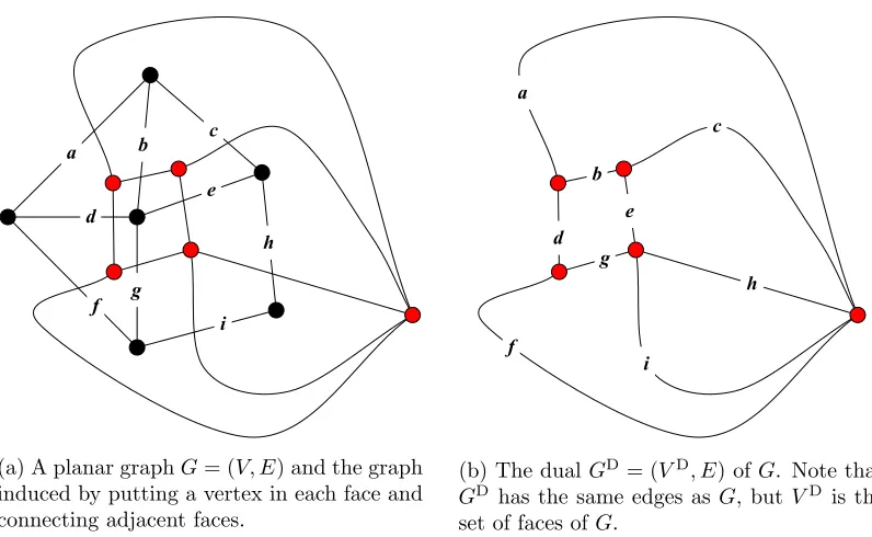
of a base in the original. The dual of the dual is, of course, the original matroid. In the case of a planar graph, the dual corresponds to the usual definition. See Fig. 1. Some additional facts about the dual (proofs omitted):
1. A circuit C in M is aco-circuit inMD and vice-versa. In the case of graphs, co-circuits are cutsets. For example, h, i and b, d, g, e are cycles inGD in Fig. 1 and they are cutsets in G. Conversely,a, c, h, i, f is a cycle inGand a cutset inGD.
2. Contraction in the dual corresponds to deletion in the original and vice versa. Contracting an edge in the dual of a planar graph has the effect of coalescing the adjoining faces, i.e., deleting the edge in the original.
3. The dual of a graphic matroid is also graphic if and only if the underlying graph is planar.
These facts have important algorithmic consequences.
First, another theorem.
Theorem 3 If C is a circuit of a matroid M = (S,B) and D is a circuit in MD, also called a
co-circuit, then |C∩D| 6= 1.
Using Theorem 3 you can show that ifxis a maximum cost element of a circuit, then there exists a minimum cost base that does not includex. So another greedy minimum spanning tree algorithm involves repeatedly finding maximum cost edges in circuits and removing them until the result is a tree. An efficient algorithm based on this idea is a randomized one by Karger et al. [23]. If we “dualize” the circuit element removal algorithm – deletion in the original corresponds to contraction in the dual – we get a version of Greedy-Min-Costthat finds the maximum weight complement of a spanning tree/forest.
Even more important algorithmically is that the circuit removal algorithm, when applied to the dual of a graphic matroid yields an algorithm that repeatedly chooses a minimum cost edge of a cut set, the underlying framework of most of the known minimum spanning tree algorithms.
You might think this works only for planar graphs. Not true: co-circuits in a graphic matroid are still cutsets of the graph. The only issue is that the dual may not be graphic.
3.2 Minors and closure properties
Aminor of a matroidM is any matroid that can be derived fromM by a sequence of deletions and contractions. Both graphic and scheduling matroids are closed under minors.
c b
d
e
f g
i h a
a
b
c
d
f
g
i e
h
(a) A planar graphG= (V, E) and the graph induced by putting a vertex in each face and connecting adjacent faces.
(b) The dual GD= (VD, E) of G. Note that
GD has the same edges as G, but VD is the set of faces ofG.
Figure 1: A planar graph and its dual. The complement of a spanning tree in the original graph is a spanning tree in the dual and vice-versa.
a b c g h d e f i
a 1 0 0 0 0 1 0 1 0
b 0 1 0 0 0 1 1 1 1
c 0 0 1 0 0 0 1 0 1
g 0 0 0 1 0 0 0 1 1
h 0 0 0 0 1 0 0 0 1
d e f i a b c g h d 1 0 0 0 1 1 0 0 0
e 0 1 0 0 0 1 1 0 0
f 0 0 1 0 1 1 0 1 0
i 0 0 0 1 0 1 1 1 1
(a) Standard representation with respect to
B ={a, b, c, g, h}.
(b) Representation of the dual with respect toE\B.
b1, . . . , br e1, . . . , er
Ir A
The representation for the dual is
e1, . . . , er b1, . . . , br
Iq AT
For the example in Fig. 1 the two matrices with respect to base {a, b, c, g, h} are shown in Fig. 2. These matrices are no longer vertex/edge incidence matrices but they do have an interesting property: ifx∈E−B then the 1’s in the column forxcorrespond toC(x, B), i.e., the endpoints of the edges in the fundamental circuit each appear exactly twice and therefore cancel out. Contraction in a binary matroid is equivalent to deleting a column and adding it to each of the others.
An obvious generalization of a binary matroid is alinear matroid, where independence corresponds to independence of a set of vectors over any field. Linear matroids were the original concrete model on which matroid theory was built [34].
The dual of a scheduling matroid M = (S,B) is also a scheduling matroid MD = (S,BD). First assume a standard representation in which the maximum deadline is n=ρ(S). Note that if there arektasks with deadlinen, the latest deadline, and the second latest deadline isn−δthen, in the original matroid, at leastδof thektasks must be scheduled. So in the dual, at most k−δof these tasks should be scheduled. This observation leads to the following recursive definition of the dual of
M = (S,B).
• ifn= 0 thenBD={S}, i.e., all tasks have deadline m=|S|andS is the unique base
• otherwise letn−δbe the latest deadline of a task with deadline< n(ornif there are no other tasks) and let Sn={i|di=n}and letk=|Sn|
• thenMDincludes the tasks ofS
n, each with deadlinek−δ, plus the dual ofM = (S0,B0), where
S0 =S\Sn andB0 ={B∩S0|B∈ B}, with k−δadded to each deadline
This process corresponds to the scheduling algorithm presented earlier, which we can now interpret as finding a minimum profit base in the dual by repeatedly deleting a maximum profit task from a circuit.
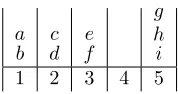
Fig. 3 illustrates the process of constructing the dual on an example. The three tasks g, h, i have deadline n and δ= 2: we give them deadline 1. Now we find the dual of the matroid with tasks
a–f: n= 3,δ= 1,Sn={e, f}; deadline is 1, but we add 1. Deadlines for the remaining tasks are determined similarly.
A more interesting example is shown in Fig. 4
a b
c d
e f
g h i
1 2 3 4 5
g h i
e f
c d
a b
1 2 3 4
The matroid M. Here, any base must have, e.g., at most one of a or b, at most two of
a, b, c, d, at least two of g, h, i and at least one of e, f if not all ofg, h, iare included.
The matroid MD. Included in any base are at least one ofa, b, at least two ofa, b, c, d, at most one of g, h, iand at most one of e, f if one ofg, h, iis included.
a b c d e
1 2 3
b c d e a
1 2
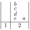
The matroidM. Any base must have at least two of b, c, d, eand may or may not havea.
The matroidMD. Because δ= 2 andk = 4 the tasks b, c, d, e are given a deadline of 2. In the reduced instancen=δ=k= 1 (only one task,a, with deadline 1). So the deadline ofain the dual is 0, which is expanded to 2.
Figure 4: Dual of a different scheduling matroid.
1
4 3 2
1
4 3 2
1
4 3 2
A transversal of size 3 A transversal of size 4 An augmenting path
Figure 5: How axiom (I3) is satisfied in a transversal matroid.
A generalization of the class of scheduling matroids istransversal matroids. LetG= (V1, V2, E) be a bipartite graph. ThenM = (V1,I), where X ⊆V1∈ I if there exists a matching that covers the vertices inX, is a transversal matroid. Clearly (I1) and (I2) are satisfied. For (I3) let X and Y be inI with|X|=|Y|+ 1 and letMX andMY be the corresponding matchings. MY must leave some vertexxofX uncovered. Observe thatMX⊕MY, the symmetric difference ofMX andMY, is the disjoint union of paths and cycles. One of the paths P must lead from x to an uncovered vertex
z∈V2. Then (MX\P)∪(MY ⊕P) is a matching that covers all ofY in addition tox. See Fig. 5
Side note: Pis usually referred to as an augmenting path. The bipartite matching problem associated with a transversal matroid can also be formulated as a max flow problem with a sources, an edge with unit capacity directed into each v ∈ V1 and a sink t with a unit capacity edge wt for each
w∈V2.
The augmenting path argument can be used for the more general class ofmatching matroids, based on non-bipartite graph matching. The corresponding flow problem is more complex. Surprisingly, it is also true that every matching matroid is also a transversal matroid – the construction is not at all obvious – so matching matroids are not really more general. A scheduling matroid is a special case of aconvex transversal matroid, one in which there exists a permutationπofV2 such that, for everyx∈V1 the set{y|xy∈E} is contiguous inπ.
a
b c d
e
f
x a
b
x
c
d
e
f
a
b c
d
e
f
(a) A graphic transversal matroid
(b) Its representation as a transversal matroid
(c) Contraction with respect to
x
is not transversal
Figure 6: A transversal matroid whose contraction with respect to a given element is not transversal.
a
b
c d
e
f
a
b
c
d
e
f
a b
e
c d
f
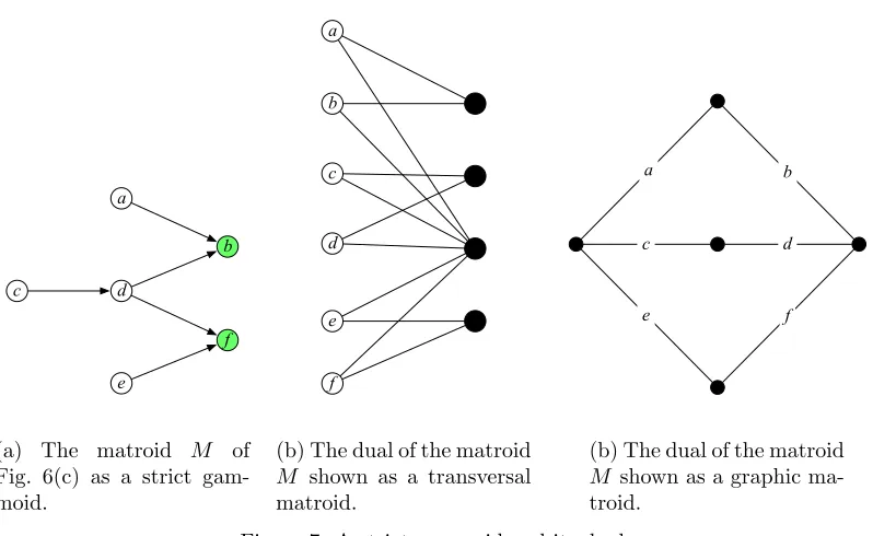
(a) The matroid M of Fig. 6(c) as a strict gam-moid.
(b) The dual of the matroid
M shown as a transversal matroid.
(b) The dual of the matroid
M shown as a graphic ma-troid.
The smallest class that includes transversal matroids and is closed under both minors and duals is the class ofgammoids, defined as follows.
• LetG= (V, E) be a directed graph andW ⊆V a fixed set of vertices.
• There is alinking ofU ⊆V into W if there is a mappingf :U 7→W such that there is a set of disjoint paths, each path leading from u∈U to f(u)∈W.
• For any fixedW the set ofU such that there exists a linking fromU intoW form the independent sets of a matroid over V. Such a matroid is called astrict gammoid.
• A gammoid is obtained by restrictingU to some subset ofV.
Fig. 7(a) illustrates the strict gammoid corresponding to the graphic matroid in Fig. 6(c). A matroid is a strict gammoid if and only if it is the dual of a transversal matroid. Proofs of this are given in the textbooks by Aigner [2] and Welsh [33]. Figures 7(b) and (c) show the dual of the strict gammoid in Fig. 7(a) as a transversal and graphic matroid respectively. It is easy to see that a transversal matroid M is a gammoid – let W be the V2 in the matching representation ofM and restrict the resulting strict gammoid to the vertices ofV1.
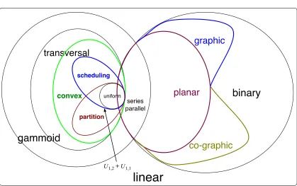
Gammoids, like binary matroids, are linear matroids. There are many ways to define a hierarchy on gammoids. Here is one. The simplest closed subclass is that of uniform matroids: Un,m is a matroid on m elements in which every subset of size n is a base. The sum of a set of uniform matroids is called a partition matroid. In general, if M1 = (S1,B1) and M2 = (S2,B2) are two matroids with S1 ∩S2 = ∅, then their sum, M1+M2, is a matroid M = (S1∪S2,B) where
B={B1∪B2 |B1 ∈ B1 andB2 ∈ B2}. A min-cost or max-profit base in a partition matroid can be found using a linear-time median algorithm.
Uniform matroids are also scheduling matroids: Un,m is equivalent to a scheduling matroid with
m tasks each having deadline n. Partition and scheduling matroids therefore agree on uniform matroids but then diverge on rank-two matroids with four elements. Let [m1, m2] denote a (rank-two) scheduling matroid with mi tasks having deadline i. A four element rank-two scheduling matroid has either six bases ([0,4] or [1,3]), five bases ([2,2] – the only non-base is the set of two deadline 1 tasks) or three bases ([3,1]). Rank-two partition matroids have six bases (U2,4), four bases (U1,2+U1,2) or three bases (U1,3+U1,1). So the scheduling matroid [2,2] cannot be a partition matroid and the partition matroidU1,2+U1,2cannot be a scheduling matroid. The only non-uniform partition matroid that is also a scheduling matroid isU1,2+U1,1
A matroidM is binary if and only if it does not have U2,4 as a minor. The “only if” part is easy:
U2,4 requires exactly two rows and four columns; in a binary matroid, one of those columns would have to be the 0 vector. A gammoid is binary if and only if it does not haveK4 as a minor, i.e., if it is the graphic matroid of a series-parallel graph.
Fig. 8 shows the relationships among the matroid classes discussed above.
4 More matroid algorithmics
Beyond finding the optimum base of a matroid there are additional, more challenging, problems, two of which are addressed here.
4.1 Matroid intersection
An instance ofmatroid intersection consists of two matroids over the same ground setM1= (S,I1) andM2= (S,I2). The objective is to findX ⊆S such that X ∈ I1∩ I2, i.e.,X is independent in both matroids. Even a maximum cardinalityX may not be trivial to find. An example of matroid intersection is bipartite matching. In contrast to the transversal matroid, the elements are the edges of a bipartite graphG= (V1, V2, E) and a set of edges must be independent in two partition matroids:
M1=
X
v∈V1
U1,deg(v)andM1=
X
v∈V2
linear
gammoid
transversal
planar
binary
uniform series parallel
graphic
co-graphic
schedulingpartition convex
U1,2+U1,1
Figure 8: A (partial) hierarchy of matroid classes (not to scale).
Here, each U1,deg(v) contains edges incident onv, i.e., at most one such edge can be included in an independent set.
Fig. 9 shows how givenmaximal matching can be extended to a maximum matching via discovery of an augmenting path. Taking the symmetric difference along the path f dehi yields matching
{a, e, f, i}. In general, a sequence of O(√n) augmenting paths leads from an empty matching to a maximum matching, as shown by Hopcroft and Karp [21].
The weighted bipartite matching problem, i.e., find a matching of maximum weight given weights on the edges, can be formulated as a linear program. Let xij = 1 if edge ij with weight wij is to be included in the matching, 0 otherwise. Here i ∈V1 and j ∈ V2. The objective is to maximize
P
ij∈Ewijxij subject to Pijxij ≤ 1 for every i ∈ V1 and Pijxij ≤ 1 for every j ∈ V2. The constraints ensure that each vertex has at most one incident edge in the matching. Early methods for solving weighted bipartite matching, sometimes known as Hungarian methods (in recognition of the K¨onig-Egervary Theorem equating maximum matching and minimum vertext cover) used the dual problem. Let yi be the dual variable corresponding to the constraint for i ∈ V1 and zj the variable for the constraint forj ∈V2. Then the objective is to minimizePi∈V1yi+
P
i∈V2zj subject
toyi+zj≥wij for every ij∈E.
The most well-known Hungarian method, as described by Lawler [25], does a sequence of breadth-first searches like the cardinality matching algorithm. The algorithm makes use of the fact that an optimum primal/dual solution is found when the followingcomplementary slackness conditions hold:
1. ifxij>0 thenyi+zj =wij
2. ifyi >0 thenPijxij = 1 (the sum is over edges incident oni)
3. ifzj>0 thenPijxij = 1 (the sum is over edges incident onj)
1 5 4 3 2 6 8 7 3 8 4 6 7 2 5 1 2 4 6 3 5
A non-maximum matching
An augmenting path
found using BFS
a
b
c
d
e
f
g
h
i
f d b i h eFigure 9: A breadth-first search finds an augmenting path with respect to a maximal matching.
4 1 2 4 6 3 5
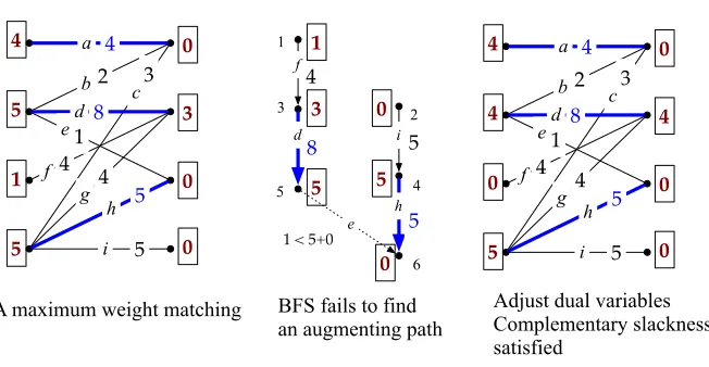
A maximum weight matching BFS fails to find an augmenting path a b d e f g h i f d i h e 4 0 3 0 0 5 1 5 5 5 4 4 1 3 2 c 8 4 1 3 0 5 5 0 1 < 5+0
8 5
5
Adjust dual variables Complementary slackness satisfied a b d e f g h i 4 0 4 0 0 5 0 4 5 5 4 4 1 3 2 c 8 4
3
6 4
2
1
c b
d
e
f g
i h a
5
a b c
d e h
f g i
1
1
2
b
f e
f i
a
d
g c
h
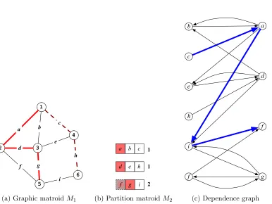
(a) Graphic matroidM1 (b) Partition matroidM2 (c) Dependence graph
Figure 11: The dependence graph for a matroid intersection and an augmenting path.
with equality. The searches for augmenting paths maintain primal and dual feasibility and (1) and (3) by starting with all xij =zj = 0 andyi= maxijwij – so (2) is not satisified until the end. An edge ij can participate in a search only if it istight, i.e., wij = xi+yj. Thus ((1) is maintained. Using auxiliary variables during the search, the algorithm, when it gets stuck, adjusts dual variables; it decreases all of theyi by a fixed amountδ, based on current conditions, and increases some, but not all of thezj byδ. Fig. 10 shows the final adjustment, after the last, unsuccessful search. The edge e, which would have been used in an augmenting path in the cardinality problem, cannot be used here because it is not tight. In this example, the first adjustment reduces all yi from 8 to 5 and increases zj to 3 only for the other endpoint of edged. This makes edges hand itight while preserving both primal and dual feasibility.
The process of augmenting and adjusting dual variables is reminiscent of many network flow algo-rithms. This is no accident – the weighted bipartite matching problem, also known as theassignment problem, is often formulated as a minimum cost flow problem.
Matroid intersection problems involving more general matroids can also be solved using variations of the augmenting paths idea. Algorithms involving intersections of graphic or scheduling matroids with partition matroids are discussed by Gabow and Tarjan [17]. The basic idea is to find a mimimum cost base (if minimum cost is the objective) followed by a sequence of swaps until the constraints of the partition matroid are satisfied, if possible.
Tong, Lawler and Vazirani [31] were able to show that matroid intersection problems on gammoids reduce to bipartite matching (in the cardinality case) and weighted non-bipartite matching, discussed below, in the weighted case. On the other side of the matroid hierarchy, more sophistication is required in the process of finding augmenting paths. As will become evident in the later discussion of matroid parity, the addition or removal of an element from either of the two matroids impacts the relationships among the other elements in nontrivial ways.
that can take place in each matroid. LetX be the current independent set and let B1 and B2 be bases inM1 andM2, respectively so thatX⊆Bifori= 1,2. Construct the (directed) dependence graphGX = (S1, S2, A) with respect to X as follows.
• create a bipartition using two copies of each matroid element, soS1=S2=S
• ify∈C(x, B1) add arcxytoA
• ifx∈C(y, B2) add arcyxtoA
The arc xy corresponding to y ∈ C(x, B1) captures the idea that, if y is removed from B1, x can replace it. The arc yx corresponding to x∈C(y, B2) captures the idea that, if y is added to B2,
x can be removed from it. A sequence of such swaps yields a path inGX; call it an augmenting path if it begins with an element y 6∈X and ends with an elementz 6∈ X. As already noted, the path may not lead to a new independent set because any swap will affect the identity of the cycles. However, Krogdahl [24] showed that an augmenting path P in the dependence graph leads to a larger independent set ifP admits no shortcuts.
Fig. 11 shows the dependence graph for a matroid intersection problem involving the intersection of a graphic matroid M1 and a partition matroid M2. The latter is U1,3+U1,3+U2,3 with sets
{a, b, c}, {d, e, h} and{f, g, i}, respectively. The current independent set X ={a, d, g}is maximal in bothM1 andM2. To turn this into a baseB1 ofM1 we add edgesc andh. To get a baseB2 in
M2 we add element f to bring the number in the partition containingg to 2. The added elements are parallel to existing ones that can replace them if an augmenting path is found. The augmenting path shown in Fig. 11(c) indicates that adding c to B2 forces the removal of a. InM1, elements
b, e and i have a in their fundamental circuits. The augmenting path suggests adding i and then removingf fromB2. Since the latter is not inX, the sequence of swaps leads to{c, d, g, i}, a larger set independent in bothM1 andM2.
For general matroids (not necessarily linear) an oracle algorithm is used in conjunction with this augmenting path idea. An oracle algorithm treats the matroid as a black box which can be queried: give it a setXand it returns the rankρ(X). Lawler [25] describes an oracle algorithm for cardinality matroid intersection that runs in time O(mn2ρ), where ρ is the time for an oracle query. This was improved to O(mn2lgn) for linear matroids by Cunningham [6]. For graphic and cographic matroids, particularly planar graphs, clever data structures can be used to keep track of cycles and the bounds are further reduced to O(mn1/2) and O(n3/2lgn) for graphic/co-graphic and planar graphs, respectively – see Gabow and Stallmann [15].
In constrast to the matching problem, formulating a linear program for the weighted case is a challenge. Instead of a simple constraint at each vertex there has to be a constraint of the form P
i∈Cxi ≤ |C| −1 for each circuit C and there are exponentially many circuits. The trick is to add these constraints on an as needed basis. Various minimum spanning tree algorithms (simple optimization, not matroid intersection) do this implicitly – see, e.g., Ahuja et al. [1]. For general matroids (not necessarily linear) an oracle algorithm is used in conjunction with the Hungarian method as described by Lawler [25] – runtime is O(mn3+mn2ρ), whereρis the time for an oracle query. For linear matroids, Frank [8] improved this to O(mM(n)), where M(n) is the time to do matrix multiplication (or, in this case, solving a system of linear equations). This can probably be improved for graphic and co-graphic matroids and especially planar graphs but the results are not in yet (as far as I know).
4.2 Matroid parity
Thematroid parity problem (sometimes calledmatroid matching) is formulated as follows: Input is a matroid M = (S,I) and a partition ofS into pairs of elements, i.e., each element x∈ S has a unique matex0 ∈ S. The objective is to find the maximum cardinality (or weight if the pairs are
weighted)X ∈ I such that, for each pairx, x0, the element x∈X if and only its matex0 ∈X, i.e.,
the pairs must stay together. A special case of matroid parity is nonbipartite graph matching. Here
M is a partition matroid composed from graphG= (V, E) asP
being a uniform matroid over the edges incident on it, but only using the half of each edge belonging to the vertex, independent of the other endpoint of the edge. Now an edge is a pair representing its two endpoints, each member of the pair participating in one uniform matroid.
Matroid parity generalizes all the problems discussed so far, as well as a large collection of network flow problems. In particular it generalizes both nonbipartite matching (and, by extension, bipartite matching) and matroid intersection. The latter is easy to see. Consider a matroid intersection problem defined byM1= (S,I1) andM2= (S,I2). LetM =M1+M2, i.e., create two copies ofS, one for each matroid, and create a pair from the two copies of each element.
Nonbipartite matching also has an augmenting path theorem: a matching is maximum if and only if it admits no augmenting path, but the situation is more complicated algorithmically than for bipartite matching. Fig. 12 illustrates how two exploratory paths in a search may meet and not yield an augmenting path even though one exists. In bipartite matching, when two paths meet, they either form an augmenting path or an even length cycle. In the latter case, either path through the cycle can be used as part of an augmenting path if one exists.
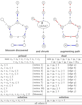
The problem in nonbipartite matching is that an “exit”, such as the one involving edgejin Fig. 12 may be missed because the alternation between matched and unmatched edges is different on oppo-site sides of the cycle. Edmonds [7] figured out that the odd cycle, which he referred to as a blossom, could simply be contracted into a single vertex, after which the search could proceed. Blossoms can also be incorporated into a linear programming formulation of the problem. In an odd cycle of length
k, at mostbk/2cedges can be included. Fig. 12 shows the full LP formulation with the dual variable
zβ corresponding to the blossomβ. Blossoms can be nested arbitrarily, but the search still succeeds if there is, indeed, an augmenting path. Furthermore, the LP formulation can be used to obtain an algorithm for weighted nonbipartite matching. Edmond’s O(n4) algorithm was implemented by Gabow [10] to run in time O(n3). This was further reduced to O(mn1/2) by Micali and Vazirani [28], matching (hah) the bound for the bipartite case.
Matroid parity, like matroid intersection, can be reduced to matching when the underlying matroid is a gammoid [31]. This works for both the cardinality and weighted cases.
The other side of the matroid hierarchy is much more interesting. Gary and Johnson [20] list spanning tree parity, matroid parity in graphic and/or co-graphic matroids, as an open problem. That same year2 Lovasz [26] showed that the cardinality parity problem for linear matroids could be solved in polynomial time, albeit with a high degree polynomial. Estimates range from O(m2n5) for (co-)graphic matroids3to O(n10) for linear matroids [27]. Furthermore, the algorithm does not resemble any algorithms for the problems that matroid parity generalizes. Lovasz and, independently, Jensen and Korte [22], also gave an exponential lower bound for any oracle algorithm solving the matroid parity problem; contrast this with matroid intersection.
As with all the special cases of matroid parity, there is an augmenting path theorem. The primary issue is how to ensure that an augmenting path, if one exists, may be found using a search.
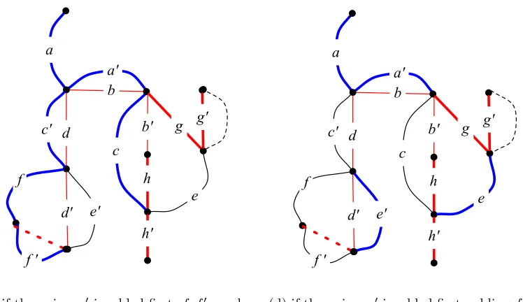
To get an idea of the pitfalls when solving the graphic matroid parity problem consider the example in Fig. 13. A standard breadth-first labeling starting atadetermines that eithercorecan be added whenb0is removed. Thenc0 forces removal ofdande0 forces removal ofd0. How the search proceeds depends on which ofc or eis encountered first. But regardless, the option of removing g, g0 after addingboth c andeis missed.
There is no obvious shrinking operation here. Instead, the solution is to create atransformT(b0, c, e) that captures all feasible exits from the blossom. In a standard representation of the binary matroid, let [zb0zgzh] be the projection onto the subspace induced byb0, g, h. Thenc= [101] (its fundamental
cycle includesb0andh) ande= [111] (the cycle includes all three). T(b0, c, e) = [101]⊕[111] = [010],4
2Actually it was a year earlier, but not well known outside of Hungary.
3Based on a Lisp implementation by Stallmann, which may still be available in electronic form if anyone really,
really wants it.
2
5 4
1
3
i h
f d j
b a
7
c
e
6 g
10 8 2
9
1
3,4,5,6,7
i h j b a
blossom discovered and shrunk
10 8
2
9
5 4
1
3
i h
f d j
b a
7
c
e
6 g
augmenting path β
primal dual
maxxa+xb+xc+xd+xe+xf miny1+y2+y3+y4+y5+y6 +xg+xh+xi+xj +y7+y8+y9+y10+ 2zβ
xa ≤1 (vertex 1) y1+y2≥1 (edgea)
xa+xb ≤1 (vertex 2) y2+y3≥1 (edgeb)
xb+xc+xd≤1 (vertex 3) y3+y4+zβ ≥1 (edgec)
xc+xe+xj ≤1 (vertex 4) y3+y5+zβ ≥1 (edged)
xd+xf ≤1 (vertex 5) y5+y7+zβ ≥1 (edgef)
xe+xg≤1 (vertex 6) y4+y6+zβ ≥1 (edgee)
xf+xg+xh≤1 (vertex 7) y6+y7+zβ ≥1 (edgeg)
xh+xi≤1 (vertex 8) y7+y8≥1 (edgeh)
xi≤1 (vertex 10) y8+y10≥1 (edgei)
xj ≤1 (vertex 9) y4+y9≥1 (edgej)
xc+xd+xe+xf+xg≤2 (blossom)
solution solution
xa =xd=xg =xj= 1 y8=y9=zβ= 1 all others 0
a
a'
b
h
b'
c
g
e
d
c'
d'
e'
f
f '
h'
g'
a' a
b' b
c'
c e
e'
d' d
f
f' g'
g
T
(
b',c,e
)
(a) an instance of graphic matroid parity; el-ements with thick, straight red lines are in-cluded in the current independent set
(b) the search for an augmenting path en-counters a classic blossom situation
a
a'
b
h
b'
c
g
e
d
c'
d'
e'
f
h'
g'
f '
a
a'
b
h
b'
c
g
e
d
c'
d'
e'
f
h'
g'
f '
(c) if the pair c, c0 is added first,f, f0 can be added, but the pairg, g0is ignored completely
(d) if the paire, e0is added first, addingf, f0
is not possible and the pairg, g0 is “blocked”
matroid class
optimization (greedy)
cardinality intersection
cardinality parity
weighted intersection
weighted parity
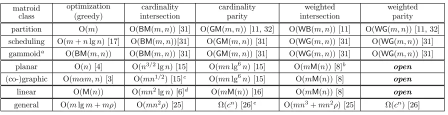
partition O(m) O(BM(m, n)) [31] O(GM(m, n)) [11, 32] O(WB(m, n)) [11] O(WG(m, n)) [11, 32] scheduling O(m+nlgn) [17] O(BM(m, n))[31] O(GM(m, n)) [31] O(WG(m, n)) [31] O(WG(m, n)) [31] gammoida O(BM(m, n)) O(BM(m, n)) [31] O(GM(m, n)) [31] O(WG(m, n)) [31] O(WG(m, n)) [31]
planar O(n) [4] O(n3/2lgn) [15] O(mnlg6
n) [15] O(mM(n)) [8]b open
(co-)graphic O(mαm, n) [3] O(mn1/2) [15]c O(mnlg6
n) [15] O(mM(n)) [8] open
linear O(M(n)) O(mn2lgn) [6]d O(mM(n)) [16] O(mM(n)) [8] open
general O(mlgm+mρ) O(mn2ρ) [25] Ω(cn) [26]e O(mn3+mn2ρ) [25] Ω(cn) [26]
aTime bounds for transversal/matching matroids extend to gammoids. bThere must be a better algorithm
cThis bound applies if m ∈ Ω(n3/2lgn). If m ∈ Ω(nlgn)∩O(n3/2lgn) the bound is O(m2/3nlg1/3n). If
m∈O(nlgn) it is O(m1/3n4/3lg2/3n).
dImproved to O(mn1.62) – don’t ask – by Gabow and Xu [19]
eHerec= 2−for→0 asn→ ∞; uses an extension of the non-linear Vamos-Higgs matroid.
Table 1: Time bounds for various matroid related algorithms; some of these may be outdated. Here m is the number of elements and n the rank of the matroid. To indicate provenance of the time bounds, let M(n), BM(m, n), WB(m, n), GM(m, n) and WG(m, n) represent the bounds for matrix multiplication, bipartite matching, weighted bipartite matching, non-bipartite matching and weighted non-bipartite matching, respectively. The notationρ, in context of time bounds for general matroids, refers to the time to query a rank or independence oracle.
which is exactlyg as desired. It also captures the fact thathis not an option.
An algorithm that solves the matroid parity problem using blossom shrinking with transforms is reported by Gabow and Stallmann [16]; it has time bounds O(mM(n)) for linear matroids and O(mn2) for (co-)graphic matroids. Using clever data structures the bound for (co-)graphic matroids can be improved to O(mnlg6n) [15].
Another line of attack on matroid parity involves a reduction to a sequence of matroid intersection problems, originally proposed by Orlin and VandeVate [30] and improved by Orlin [29]. Time bounds are O(mn4) and O(m3n), respectively, for linear matroids.
In Table 1 gives the latest bounds (as far as I know) for algorithms solving a wide variety of matroid problems. Some of the entries depend on the following time bounds, also subject to improve-ment.
• matrix multiplication,M(n)∈O(n2.2...), Coppersmith and Winograd [5].
• cardinality bipartite matching,BM(m, n)∈O(mn1/2), Hopcroft and Karp [21].
• cardinality nonbipartite matching, GM(m, n)∈O(mn1/2), Micali and Vazirani [28].
• weighted bipartite matching,WB(m, n)∈O(mn+n2lgn), Fredman and Tarjan [9].
References
[1] Ravindra K. Ahuja, Thomas L. Magnanti, and James B. Orlin. Network Flows: Theory, Algo-rithms, and Applications. Prentice Hall, 1993.
[2] Martin Aigner. Combinatorial Theory. Springer, 1979.
[3] Bernard Chazelle. A minimum spanning tree algorithm with inverse-Ackermann type complex-ity. JACM, pages 1028–1047, 2000.
[4] David Cheriton and Robert E. Tarjan. Finding minimum spanning trees. SIAM J. Computing, pages 724–742, 1976.
[5] D. Coppersmith and S. Winograd. Matrix multiplication via arithmetic progressions. Journal of Symbolic Computation, pages 251–280, 1990.
[6] William H. Cunningham. Improved bounds for matroid partition and intersection algorithms. SIAM J. Computing, pages 948–957, 1986.
[7] Jack R. Edmonds. Paths, trees and flowers. Canadian J. Math., pages 449–467, 1965.
[8] Andr´as Frank. A weighted matroid intersection algorithm. J. Algorithms, pages 328–336, 1981.
[9] Michael L. Fredman and Robert E. Tarjan. Fibonacci heaps and their uses in improved network optimization algorithms. JACM, pages 596–615, 1987.
[10] Harold N. Gabow. An efficient implementation of edmonds’ algorithm for maximum matching on graphs. J. ACM, 23(2):221–234, April 1976.
[11] Harold N. Gabow. An efficient reduction technique for degree-constrained subgraph and bidi-rected network flow problems. InProc. 15th Ann. ACM Symp. on Theory of Computing, 1983.
[12] Harold N. Gabow. Data structures for weighted matching and nearest common ancestors with linking. InProc. First Ann. Symp. on Discrete Algorithms, 1990.
[13] Harold N. Gabow, Zvi Galil, and Thomas H. Spencer. Efficient implementation of graph algo-rithms using contraction. JACM, pages 540–572, 1989.
[14] Harold N. Gabow, Zvi Galil, Thomas H. Spencer, and Robert E. Tarjan. Efficient algorithms for finding minimum spanning trees in undirected and directed graphs. Combinatorica, pages 109–122, 1986.
[15] Harold N. Gabow and Matthias F. Stallmann. Efficient algorithms for graphic matroid inter-section and parity. InAutomata, Languages and Programming, number 194 in Lecture Notes in Computer Science, 1985.
[16] Harold N. Gabow and Matthias F. Stallmann. An augmenting path algorithm for linear matroid parity. Combinatorica, pages 123–150, 1986.
[17] Harold N. Gabow and Robert E. Tarjan. Efficient algorithms for simple matroid intersection problems. Journal of Algorithms, pages 80–131, 1984.
[18] Harold N. Gabow and Robert E. Tarjan. A linear-time algorithm for a special case of disjoint set union. J. Comp. and Syst. Science, pages 209–221, 1985.
[19] Harold N. Gabow and Ying Xu. Efficient theoretic and practical algorithms for linear matroid intersection problems. J. Comp. and Syst. Sci., pages 129–147, 1996.
[21] John E. Hopcroft and Richard M. Karp. Ann5/2algorithm for maximum matchings in bipartite graphs. SIAM J. Computing, pages 225–231, 1973.
[22] Per M. Jensen and Bernhard Korte. Complexity of matroid property algorithms. SIAM J. Computing, pages 184–190, 1982.
[23] David R. Karger, Philip N. Klein, and Robert E. Tarjan. A randomized linear-time algorithm to find minimum spanning trees. JACM, pages 321–328, 1995.
[24] Stein Krogdahl. The dependence graph for bases in matroids. Discrete Mathematics, 19(1):47– 59, 1977.
[25] Eugene L. Lawler. Combinatorial Optimization: Networks and Matroids. Holt, Rinehart and Winston, 1976.
[26] L´azl´o Lov´asz. The matroid matching problem. InAlgebraic Methods in Graph Theory, Colloquia Mathematica Societatis J´anos Bolyai, pages 495–517, 1978.
[27] L´azl´o Lov´asz and M. D. Plummer. Matching Theory. North Holland, 1986.
[28] Silvio Micali and Vijay V. Vazirani. AnO(p|V||E|) algorithm for finding maximum matchings in general graphs. InProc. 21st Ann. Symp. on Foundations of Computer Science, 1980.
[29] James B. Orlin. A fast, simpler algorithm for the matroid parity problem. InInteger Program-ming and Combinatorial Optimization, volume 5035 of Lecture Notes in Computer Science, pages 240–258, 2008.
[30] James B. Orlin and John H. VandeVate. Solving the matroid parity problem as a sequence of matroid intersection problems. Mathematical Programming, pages 81–106, 1990.
[31] Po Tong, Eugene Lawler, and Vijay V. Vazirani. Solving the weighted parity problem for gammoids by reduction to graphic matching. InProgress in Combinatorial Optimization, pages 363 – 374. Academic Press, 1984.
[32] Robert J. Urquhart. Degree constrained subgraphs of linear graphs. PhD thesis, University of Michigan, 1967.
[33] D.J.A Welsh. Matroid Theory. Academic Press, 1976.
[34] Hassler Whitney. On the abstract properties of linear dependence. American Journal of Math-ematics, pages 509–533, 1935.
Acknowledgement