DOI 10.1007/s10844-011-0183-2
Community-based anomaly detection
in evolutionary networks
Zhengzhang Chen·William Hendrix· Nagiza F. Samatova
Received: 7 March 2011 / Revised: 2 August 2011 / Accepted: 6 October 2011 © Springer Science+Business Media, LLC 2011
Abstract Networks of dynamic systems, including social networks, the World Wide
Web, climate networks, and biological networks, can be highly clustered. Detecting clusters, or communities, in such dynamic networks is an emerging area of research; however, less work has been done in terms of detecting community-based anomalies. While there has been some previous work on detecting anomalies in graph-based data, none of these anomaly detection approaches have considered an important property of evolutionary networks—their community structure. In this work, we present an approach to uncover community-based anomalies in evolutionary net-works characterized by overlapping communities. We develop a parameter-free and scalable algorithm using a proposed representative-based technique to detect all six possible types of community-based anomalies: grown, shrunken, merged, split, born, and vanished communities. We detail the underlying theory required to guarantee the correctness of the algorithm. We measure the performance of the community-based anomaly detection algorithm by comparison to a non–representative-community-based algorithm on synthetic networks, and our experiments on synthetic datasets show that our algorithm achieves a runtime speedup of11–46over the baseline algorithm. We have also applied our algorithm to two real-world evolutionary networks, Food Web and Enron Email. Significant and informative community-based anomaly dynamics have been detected in both cases.
This work was supported in part by the U.S. Department of Energy, Office of Science, the office of Advanced Scientific Computing Research (ASCR) and the Office of Biological
and Environmental Research (BER) and the U.S. National Science Foundation (Expeditions in Computing). Oak Ridge National Laboratory is managed by UT-Battelle for the LLC U.S. D.O.E. under contract no. DEAC05-00OR22725. Z. Chen·W. Hendrix·N. F. Samatova (
B
)Department of Computer Science, North Carolina State University, Raleigh, NC 27695, USA e-mail: samatova@csc.ncsu.edu
Z. Chen·N. F. Samatova
Keywords Anomaly detection·Time-varying graphs·Evolutionary analysis· Community detection·Community-based anomaly
1 Introduction
As opposed to most research in anomaly detection, which is based on strings or attribute-value data as the medium, graph-based anomaly detection focuses on data that can be represented as a graph (Noble and Cook2003). It has provided new ap-proaches for handling data that can’t be easily analyzed with traditional non–graph-based data mining approaches (Noble and Cook2003) and has found applications in several domains. One of the most important of these areas is intrusion detection. GrIDS, a graph-based intrusion detection system, was developed by Staniford-chen et al. (1996). Padmanabh et al. (2007) proposed a random walk-based approach to detect outliers in Wireless Sensor Networks. Eberle and Holder (2006) focused on detecting anomalies in cargo shipments. Noble and Cook (2003) used anomaly detec-tion techniques to discover incidents of credit card fraud (Eberle and Holder2007).
Graph-based anomaly detection has been studied from two major perspectives: “white crow” and “in-disguise” anomalies. Intuitively, a “white crow” anomaly (also called an “outlier” in many papers) is an observation that deviates substantially from the other observations (Moonesinghe and Tan2006), while an “in-disguise” anomaly is only a minor deviation from the normal pattern (Eberle and Holder
2007), as shown in Fig.1. For example, if we are analyzing the voters list and we come across a person whose age is 322, then we can take that as a “white crow” anomaly, because the age of a voter will typically lie between18and100. On the other hand, anyone who is attempting to commit credit card fraud would not want to be caught—a criminal would want his or her activities to look as normal as possible, which represents an “in-disguise” anomaly. Anomalies classified as “white crow” are usually detected as nodes, edges, or subgraphs, while “in-disguise” anomalies are now only identified through unusual patterns, including uncommon nodes or entity altera-tions. A summary of the various research directions in this area is shown in Fig.2.
Fig. 1 “White crow” and
“in-disguise” anomalies
1 2 3 4 5 6 7 6
5
4
3
2
1
In-disguise
Research on Graph -based Anomaly Detection
“White Crow” Anomaly Detection
“In-disguise” Anomaly Detection
Type of Anomalies Type of Anomalies
Nodes Edges Substructures Entity
Alterations Nodes
Simple Graph: Random Walk [Moonesinghe 2006]
Bipartite Graph : Relevance Search
[Sun 2005] kNN Graph:
Density-based Method [Hautamaki 2004]
Minimum Description Length Principle
[Chakrabarti 2004]
Subdue-based Method [Noble 2003]
Rarity Measurement
[Lin 2003] Tensor -based
Method [Sun 2006]
Minimum Description Length Principle [Eberle 2007]
Event -based Entropy
Model [Shetty 2005]
Fig. 2 A summary of the various research directions in graph-based anomaly detection
Research on “white crow” anomaly detection has traditionally focused on ex-ploring three different types of anomalies. Aiming to identify anomalous nodes, Moonesinghe and Tan (2006) proposed a random walk–based approach that rep-resents the dataset as a weighted undirected graph. Similarly, an algorithm based on random walks with restarts was used by Sun et al. (2005) for relevance search in an unweighted bipartite graph, in which vertices with low normality scores were treated as anomalies. Hautamäki et al. (2004) took a different approach and applied two density-based outlier detection methods to discover novelty vertices in a k-nearest
neighbour graph. To identify unusual edges, Chakrabarti (2004) used the minimum
system. In contrast to Noble and Cook (2003), Lin and Chalupsky (2003) applied rarity measurements to discover unusually linked entities within a labeled directed graph.
Unlike the previously mentioned single graph algorithms, Cheng et al. (2008) provided a robust algorithm for discovery of anomalies in noisy multivariate time series data. To deal with higher order data, Sun et al. (2006) introduced a tensor-based approach. Other related work on “white crow” anomaly detection can be found in Chan and Mahoney (2005), Sun et al. (2007), Keogh et al. (2005) and others.
“In-disguise” anomalies are more difficult to detect because they are highly hidden in the graph, and less work has been reported on detecting such anomalies. Eberle and Holder (2007) introduced three algorithms based on the minimum description length principle for the purpose of detecting three categories of anomalies that closely resemble normal behavior, including label modifications, vertex/edge inser-tions, and vertex/edge deletions. In addition, Shetty and Adibi (2005) exploited an event-based entropy model that combines information theory with statistical tech-niques to discover hidden prominent people in an Enron e-mail dataset. However, none of these work is focused on detecting “in-disguise” anomalies in multiple graphs. Meanwhile, neither “white crow” nor “in-disguise” anomaly detection approaches have considered one of the important properties of evolutionary networks: their community structure, which is sometimes referred to as clustering (Girvan and Newman2002).
Networks of dynamic systems can be highly clustered (Watts and Strogatz1998). A community, defined as a collection of individual objects that interact unusually frequently, is a very common substructure in many networks (Girvan and Newman
2002), including social networks, metabolic and protein interaction networks, financial market networks, and even climate networks. In social networks, a commu-nity is a real social grouping sharing the same interests or background (Girvan and Newman2002). In biological networks, a community might represent a set of proteins that perform a distinct function together. Communities in financial market networks might denote groups of investors that own the same stocks, and communities in climate networks might indicate regions with a similar climate or climate indices.
Many algorithms have been developed for detecting community structures in static graphs. Girvan and Newman (2002) proposed a community discovery algo-rithm based on the iterative removal of edges with high betweenness scores. To reduce the computational cost of the betweenness-based algorithm, Clauset et al. (2004) proposed a modularity-based algorithm. In contrast, Palla et al. (2005) did not focus on detecting separate communities, but on finding overlapping communities. Defining communities as maximal cliques, Schmidt et al. (2009) proposed a parallel, scalable, and memory-efficient algorithm for their enumeration.
Communities in real networks change over time, and being able to detect small community deviations can help us understand and exploit these networks more effectively. For example, in biological networks, a small variation in a gene-gene association community may represent an event, such as gene fusion (Snel et al.
2000), gene fission (Snel et al.2000), gene gain (Chen et al.1997), gene decay (Long et al. 2003), or gene duplication (Zhang2003), that would change the properties of the gene products (e.g., proteins) and, consequently, affect the phenotype of the organism. Interesting community deviation patterns in Food Web and social networks are discussed in Section3.
Thus, in contrast to the previous work on identifying communities or tracking conserved communities, we focus on detecting community-based anomalies, a new type of “in-disguise” anomalies, in dynamic networks. Specifically, our work pro-poses the novel problem of detecting these “in-disguise” anomalies across multiple dynamically evolving graphs, or evolutionary networks, for short. Our approach follows from the need to address the following four challenges:
– How do we define community-based anomalies, and how many types of
community-based anomalies are possible in evolutionary networks? From an anomaly detection perspective, we are interested in dynamic, abnormal com-munities that would reveal novel properties of the network, as opposed to conserved communities or communities at a single snapshot. For example, is there a community at snapshot t that splits into smaller communities or merges with others at snapshot t+t? Does any community at snapshot t disappear at snapshot t+t, or does any new community appear at snapshot t+t? Do the sizes of the communities change over time?
– Most real networks are dynamic and characterized by overlapping communities (Palla et al.2005). Detecting dynamic communities from networks characterized by overlapping communities is more challenging than discovering communities in static networks.
– How do we detect community-based anomalies across multiple dynamically evolving networks? As we mentioned earlier, real-world networks change over time, requiring us to adopt evolutionary analysis techniques to detect such anomalies.
– Since there may be hundreds or even thousands of communities in each real-world network, how to scale a community-based anomaly detection algorithm to large graphs?
In this paper, we propose solutions to all four of these problems. Our algo-rithm is based on the proposed notion of graph representatives and community representatives. Graph representatives helps us reduce the expensive computational cost of enumerating communities, which we model as maximal cliques, whereas community representatives is utilized to identify community-based anomalies.
The contributions of our work are:
1. We identify a new type of anomaly—the community-based anomaly in complex evolutionary networks.
3. We prove that there are only six possible types of community-based anomalies in dynamic simple undirected graphs.
4. We develop a community-based anomaly detection algorithm based on graph representatives and community representatives.
5. We evaluate our method on real datasets to confirm its applicability in practice. The rest of the paper is organized as follows: Section2introduces some necessary definitions and formally defines the problem. In Section 3, we show application of community-based anomaly detection to two real-world dynamic networks, Food Web and Enron Email. Section4presents the community-based anomaly detection algorithm. In Section 5, we evaluate the algorithm with synthetic data. Finally, Section6concludes the paper.
2 Problem statement
In this paper, the ultimate goal is to find community-based anomalies in dy-namic graphs, and our algorithm is based on graph representatives and community representatives. Thus, the following terms and problems need to be addressed. The symbols used in the paper are listed in Table1.
Problem 1 (Community-based anomaly detection) Given a time-varying sequence
of undirected simple graphsG= {G1,G2,G3, ...}, where the nodes in each graph can
belong to different communities, detect the community-based anomalies between consecutive graphs, including grown, shrunken, merged, split, born, and vanished communities (see Definition 7).
Definition 1 (Community) Communities are the maximal cliques in a graph.
There is no formal definition for the community structure in a network (Girvan and Newman2002). The simplest and the most conservative definition of a
commu-Table 1 Symbol table
Symbol Description
Gi A simple undirected labeled graph
G A sequence of graphs
Ci
t The community of index i in graph Gt
Rep(Gi) The representative node set of graph Gi Ci
t→C j
t+1 Citis a predecessor of C j t+1, or C
j
t+1is a successor of Cit V(Ci
t) The node set of community Cit
SV(Gi) Common nodes between graphs Giand Gi+1
|C| The size of community C
T The number of timestamps in the sequence
|V(C)| The number of vertices in community C
vj A vertex j in a graph
CGi The list of communities in Gi
VCivj The list of communities that contain nodevjin graph Gi Checked(Gi) The list of nodes in Githat have been checked
nity is a clique, a set of vertices that are pairwise adjacent to one another. Another definition used by Girvan and Newman (2002) is a dense subgraph, a group of vertices within which the connections are denser than between different groups (Girvan and Newman2002).
As our goal is to detect abnormal, changing communities, we propose to use the more specific community definition, namely clique. From an application perspective, we could lose important information if we shifted to dense subgraphs as communi-ties. For example, consider protein functional modules (biological communities) in protein-protein interaction networks. Across different organisms, such evolutionary networks might have undergone small changes, or perturbations, due to evolutionary events such as gene fusion, gene fission, gene gain, gene decay, or gene duplica-tion. Relatively small perturbations to the network structure due to the genotype variation may induce phenotype variations, such as organism’s capability to produce hydrogen or ethanol, to resist high temperature, to fix nitrogen, etc. Since network perturbations could be infinitesimal, considering communities as dense subgraphs with respect to some density parameter, may arguably be insufficient for capturing such fine-grain changes to the network structure. Therefore, we propose to use the simplest, the most stringent, and parameter-free definition of a community—a clique. We use the maximal clique, i.e., a clique that can’t be extended by adding any more vertices in order to decrease the space of putative anomaly-based communities to evaluate and thus to reduce the overall computational cost.
Definition 2 (Community size) The community size,|C|, is the number of vertices in the community, so|C| = |V(C)|.
Definition 3 (Graph representative) Representatives of graph Giare the nodes that also appear in Gi−1, Gi+1, or both. Thus, Rep(Gi)= {vi|vi∈V(Gi)∩(V(Gi−1)∪
V(Gi+1))}.
Nodes that only appear in one graph are called graph-specific nodes or vertices.
Definition 4 (Graph-specific community) A graph-specific community is a
commu-nity that does not contain any graph representative.
Since our goal is to detect community-based anomalies, we do not try to discover graph-specific communities. Thus, by using graph representatives as seeds, we do not need to enumerate all communities in the graphs, only those communities that contain graph representatives, and thus potentially reducing computational time (see Section4for details).
Definition 5 (Community predecessor and successor) If community Ci
tat snapshot
t is a subset or superset of community Ctj+1at snapshot t+1, then the community Cit
is a predecessor of Ctj+1, and C j
t+1is a successor of Cit. This relationship is denoted by
Cti→C
j t+1.
Definition 6 (Community representative) A community representative of Ci t is a node in Ci
same graph. If there is more than one node that satisfies this condition, we choose one at random.
The rationale for our definition of a community representative follows from the observation that the community Ci
tcan be represented by a node that only appears in community Ci
t. However, since the communities in our networks may be highly overlapping, we cannot guarantee that such a node exists, so we look for a node in Ci
t that has the minimum number of appearances in other communities to use as its representative. In this way, we limit the nodes that belong to more than one community from being a community representative, which helps to establish the relationships between the communities (see Section4for details).
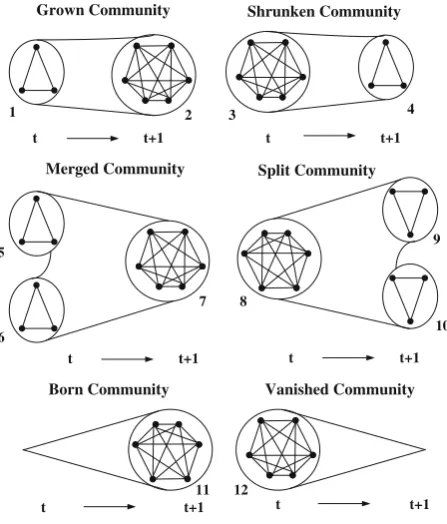
Definition 7 (Community-based anomalies) In contrast to Palla et al. (2007), which focuses on the stability/stationarity of the communities, our goal is to detect community-based anomalies. As there are six basic events that may occur to a community (Palla et al.2007), we can define six possible types of community-based anomalies in evolutionary networks (see Fig.3).
1. Grown community
In real-world networks, some “big” communities, like community 2, can be grown from previous “smaller” communities by adding some new members. These “big” communities are called grown communities.
Fig. 3 Possible types of
community-based anomalies in evolutionary networks
Grown Community
t t+1
Shrunken Community
t t+1
t t+1
t t+1 t t+1
t t+1
Merged Community Split Community
Born Community Vanished Community
1 2 3 4
5
6
7 8
9
10
2. Shrunken community
On the other hand, shrunken communities, like community4, are communities caused by previous “bigger” communities losing some members.
3. Merged community
In addition, two or more “small” communities at snapshot t often join together to form one merged community, like community7, at snapshot t+1.
4. Split community
Meanwhile, a split community at snapshot t, like community8, may break up into multiple communities at snapshot t+1.
5. Born community
What’s more, some “new” communities, like community11, may appear in some snapshots, but born communities should contain at least one graph representa-tive in order to avoid considering graph-specific communities as anomalies.
6. Vanished community
Alternatively, some “old” communities, like community 12, may disappear. Similar to born communities, vanished communities should contain at least one graph representative to exclude graph-specific communities.
Evolutionary network conservation, which is often manifested with stable com-munities that do not change over time, is a well-recognized property of many real-world complex dynamic networks. For example, in climate networks, such communities may correspond to well-known climate indicies. Likewise, in biological networks, such stable communities may correspond to protein complexes, such as ATP synthase or ribosomal machinery, and metabolic pathways, such as TCA cycle. In contrast to stable communities, an anomalous community is often highly hidden among an enormous number of stable communities in evolutionary networks. In real-world networks, like social networks, a majority of people’s friendship communities tend to be stable despite frequently occuring changes in individuals’ activities and communication patterns (Palla et al.2007).
It is often the case, especially if t is small, that only very few communities might slighly change due to some anomalous events. For example, resignation of the CEO in a company may induce changes to community composition, if community membership is defined by email communication traffic between a sender and a receiver. Likewise, in climate networks, the seasons of unusually high hurricane activity are likely induced by changes in climate communities found in the climate networks for the seasons with low hurricane activity. Thus, rare and anomolous events are likely caused by or induce structural changes in the communities, and result in the appearance of anomalous communities. Such anomalous communities often overlap with other “normal” (or stable) communities, which makes it even more difficult to distinguish between normal and anomolous communities. Thus, community-based anomaly can be seen as a new type of “in-disguise” anomaly.
3 Application of community-based anomaly detection to real-world dynamic networks
Table 2 Food Web communities
Season Number of Abnormal communities communities
Spring 15 None
Summer 15 Four grown communities, one born community, four communities will split in fall, one vanished community, and one merged community Fall 19 Two shrunken communities and four vanished communities
(will disappear in winter) Winter 9 Four merged communities
Food Web and Enron Email. In this section, we consider only communities of size three or more.
Food Web dataset The Food Web dataset, which was originally compiled by Baird and Ulanowicz (1989), consists of marine organisms living in the Chesapeake Bay, containing33 vertices that represent the ecosystem’s most prominent taxa. Edges
Phytoplank ton Bacteria Oysters
Zoo plankton
Other suspen feeders
Mya
Spring Summer
phytoplank ton Bacteria Oysters
Zoo plankton
Other suspen
feeders Mya
Micro zooplank
Alewif&blue herring Striped
bass
Bay anchovy
Menhaden
Zoo plankton
Summer Fall
Alewif&blue herring Striped
bass
Bay anchovy
Menhaden
Zoo plankton
Shad
Grown Communities:
Shrunken Communities:
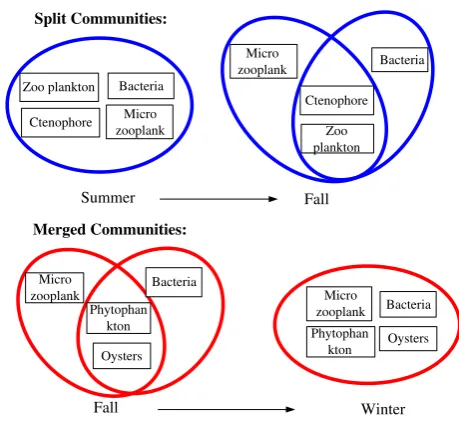
Fig. 5 Example of a split
community and a merged community in Food Web
Summer Fall
Bacteria Zoo plankton
Micro zooplank
Fall Winter
Merged Communities: Split Communities:
Ctenophore
Bacteria
Zoo plankton Micro
zooplank
Ctenophore
Bacteria
Oysters Micro
zooplank
Phytophan kton
Bacteria
Oysters Phytophan
kton Micro zooplank
between taxa denote trophic relationships—one taxon feeding on another. Here, we ignore directionality and consider the network as an undirected graph. Girvan and Newman (2002) has used this dataset as a static graph to detect the communities, while we construct the networks on a seasonal basis from spring to winter to discover community-based anomalies in the dynamic network.
By applying our algorithm to the Food Web networks, we find instances of all six types of community-based anomalies (see Table2). Summer is the most active community changing season: four communities grow because microzooplankton, which cannot be found in Spring, become involved in the energy flow network. Four communities split because bacteria do not feed on microzooplankton in Fall. The disappearance of sea nettle in the Fall results in a vanished community (zooplankton, ctenophore, and sea nettle). This community was a born community in Summer, indicating that it is unstable. Due to a lack of food in Winter, four communities merge in order to benefit from more members with food energy. Typical community-based anomaly examples discovered in Food Web are shown in Figs.4,5and6. Note that
Spring Summer
Sea nettle Ctenophore
Zoo plankton
Bay anchovy
Menhaden Blue fish
Fall Winter
Born Community: Vanished Community:
Table 3 Enron email dataset
properties Month Number of edges Number of communities
January 126 21
February 190 56
March 199 54
April 240 66
May 273 90
June 218 49
July 240 68
August 371 120
September 343 110
October 531 196
November 438 143
December 290 93
the different circles represent different communities at the same time stamp—we can see that Food Web is characterized by overlapping communities.
ENRON dataset This data set consists of approximately1.5million email
commu-nications sent or received by employees in Enron, Inc. It is much more complex than the Food Web dataset. We take a subset containing only messages between Enron employees from January to December of 2001 and construct sender-to-recipient undirected graphs on a monthly basis. The graphs have151nodes (Enron employees), with low edge density and short average distance between vertices, which shows a “small-world” effect and indicates that the graphs have community structure. The properties of each graph are shown in Table3.
The community-based anomalies in each month discovered by our algorithm are shown in Table4. We can see that there are more abnormal communities in October than in any other month. The most likely trigger of this event is the fact that Enron announced a third quarter loss of$618million on October 16 of 2001, which is also thought to be the trigger of the Enron scandal.
In order to see the details of the community-based anomalies in October, let us consider one of the most important nodes—Louise Kitchen, the former President of Enron. There are20abnormal communities containing Louise Kitchen in October:
Table 4 Community–based anomalies in enron email dataset
Month Grown Shrunken Merged Split Born Vanished
January 0 0 0 0 0 14
February 3 1 0 1 48 32
March 3 2 4 1 33 39
April 6 1 0 2 42 43
May 3 4 0 1 75 76
June 3 3 0 1 34 38
July 1 0 2 0 58 54
August 9 4 2 2 97 89
September 8 9 3 1 79 56
October 30 5 10 8 136 160
November 7 13 0 9 102 97
16 born communities, 4 grown communities, 1 split community, and 1 shrunken community. From Fig. 7, we can see that some employees like Sally Beck, Chief Operating Officer, joined the senior management communication groups, probably to discuss the serious issues or suggest strategies, while only one person—Phillip
Louise Kitchen
September October
Shrunken Community:
Grown Communities:
Rosalee Fleming Steven
Kean
Sally Beck Louise
Kitchen Greg Whalley
Andy Zipper
Jeff Dasovich
Barry Tycholiz
Phillip Allen
Louise Kitchen Jeff Dasovich
Barry Tycholiz
Greg Whalley Andy
Zipper
Louise Kitchen
Arnold John Jeffrey Shankman
Arnold John
Jeffrey Shankman Rick
Buy
September October
Sally Beck
Rick Buy
Split Community:
Louise Kitchen Jeff Dasovich
James Steffes Steven Kean Richard Shapiro
October November
Louise Kitchen
Jeff Dasovich James
Steffes Steven Kean Richard Shapiro
August September Danny
McCarty
Jeff Skilling
Stanley Horton Jeffrey
Shankman
Drew Fossum Steven
Kean
Kenneth Lay Vince Kaminski
Greg Whalley
Danny McCarty Stanley
Horton Jeffrey
Shankman
Drew Fossum Steven
Kean
Vince Kaminski
Greg Whalley
Fig. 8 Shrunken communities due to Jeff Skillng resigning as CEO in August
Allen—left the groups. Confusion among the Enron employees may be why Louise Kitchen’s communication groups grew rather than shrank during the turbulent times. As a second example, take Jeff Skilling, the former CEO of Enron. There are19 email communities contain Jeff Skilling in August, but among these, three communities shrank in September (see Fig. 8), while the other 16 communities disappeared after Jeff Skilling resigned as CEO in August, perhaps because many employees quit or joined other work groups after Skilling’s resignation.
4 Community-based anomaly detection algorithm
In this section, we discuss the proposed algorithm for solving the problem presented above. We prove some necessary lemmas and theorems in Section4.1. Then, based on the abnormal community decision rules described in Section4.2, we illustrate how to detect community-based anomalies in Section4.3.
4.1 Lemmas and theorems
We present the following theorems and lemmas to provide a sound theoretical basis for our community-based anomaly detection. Proofs for these appear inAppendix.
Lemma 1 If community Ci
t has more than one predecessor (or successor), then the
sizes of its predecessors (or successors) are either all larger thanCi
tor all smaller
thanCi
t.
Similarly, if a community Ci
t has more than one successor, then the sizes of its successors are either all larger thanCi
tor all smaller thanCit. This lemma is used to prove the following completeness result:
Theorem 1 Let Gtand Gt+1both be simple, undirected graphs, where communities
are def ined as maximal cliques. If Gt+1is the perturbed graph formed by either adding
edges/nodes to or removing edges/nodes from the baseline graph Gt, then there are
communities, shrunken communities, merged communities, split communities, born
communities, and vanished communities, as def ined in Def inition7.
Lastly, we present a theorem that will allow us to reduce the computational complexity of identifying the community-based anomalies.
Theorem 2 If community Ci
tis represented by vertexvi∈Cti, and community C
j t+1is
represented by vertexvj∈C
j
t+1, where Cit→C j
t+1, thenvi∈C j
t+1orvj∈Cit.
From Theorem 2, if there is more than one node in community Cm
t and Cnt+1that
satisfies the condition of community representative, then we can randomly choose vmto represent Cmt andvnto represent Cnt+1to help check the relationship between
Ctmand Cnt+1as follows:
1. If vm∈Cnt+1, then C n
t+1 can be detected as a potential successor to C i t. By Definition 5, the relationship Cm
t →C n
t+1 would be established if C n t+1 also
satisfies Cm
t ⊆Cnt+1or Cnt+1⊆Cmt .
2. If vm∈/Cnt+1, then by Theorem 2,vn∈C m
t if Cmt →Ctn+1. In this case, we can
detect the relationship Cm
t →Cnt+1throughvnand check whether Ctm⊃Cnt+1.
Thus, random selection of the community representative will not affect our detection results.
4.2 Abnormal community decision rules
Based on our result from Theorem 1, we can identify community-based anomalies using the following rules:
1. If community Ci
thas only one predecessor C j t−1:
(a) If the size of the predecessor is smaller than Ci
t, then Cit is a grown community.
(b) If the size of the predecessor is larger thanCi
tand Ctiis the only successor of Ctj−1, then C
i
tis a shrunken community. (c) If the size of the predecessor is larger than Ci
tand Cit is not the only successor of Ctj−1, then C
i
tis a product of the split community C j t−1.
2. If community Ci
thas more than one predecessor:
(a) If the sizes of the predecessors are all smaller thanCi
t, then Citis a merged community.
(b) If the sizes of the predecessors are all larger thanCi
tand Citis the only successor of one of its predecessors, then Ci
tis a shrunken community. (c) If the sizes of the predecessors are all larger thanCi
tand Cit is not the only successor of one of its predecessors, then that community is a split community and Ci
tis one of its products. 3. If community Ci
4.3 Algorithm description
In this section, we describe our method for detecting and tracking anomalous communities based on the proposed notion of graph representatives and community representatives.
To the best of our knowledge, the proposed problem of detecting and tracking community-based anomalies in evolutionary networks has not been addressed in literature. Thus, for comparison purposes, we first briefly describe a brute-force solution that does not use graph representatives and community representatives. Then, we provide details on how graph representatives can help reduce the expensive computational cost caused by community enumeration, and how community repre-sentatives can be utilized to effectively identify community-based anomalies.
Non-representative-based method A brute-force solution that does not use graph or community representatives is to first enumerate all communities in each graph, and then compare all possible pairs of communities belonging to consecutive timestamps. For example, to find the successors of community A in Fig.9, we need to compare community A with communities D, E, F, and K at snapshot t+1; that is, we compare community A with all communities at snapshot t+1, although only community F is the successor of A. This two-stage approach is infeasible and impractical, because of a possibly enormous number of communities to search. Among those, there are many redundant communities (e.g., graph-specific communities (see Definition 4)) in each graph, and it does not make much sense to compare pairs of communities that contain no common members or few members.
Representative-based method To reduce the computational cost, we designed an algorithm based on the graph representatives and community representatives (see Definition 3 and 6 in Section2). The workflow of the algorithm is shown in Fig.10. For each graph, we first find graph representatives (see Step 1 in Fig.10) and enumer-ate the communities that are seeded by the graph representatives to avoid generating graph-specific communities (see Step 2 in Fig.10). We call these communities seed-communities. In every seed-community, we select only one node as a community representative (see Step 3 in Fig.10) and use community representatives to establish
A
B
C
F
E D
t t+1
H J
t+2
1 1
2
3 3
3
4 4
4
5 5 5
6 6 6
7
7
13
12
10 10
8 7 8
9 9
11 11
8 14 15 16
18 19 20
I K
21 23 22
L G
24
25 M
2
Fig. 9 Example for tracking community-based anomalies using the non–representative-based
Fig. 10 Workflow of the
community-based anomaly detection algorithm
Sequence of Dynamic Graphs
t t+1
Step 1: Identify
Step 2: Emumerate
1 2 3 1 6 5 3 2 t+2 2 1 3 5 6 4 9
t t+1 t+2
8
Step 4: Establish
Step 5: Detect
t+1 Born Community: Grown Community: 7 Graph Representatives t t+1 1 2 3 1 6 5 3 2 t+2 2 1 3 5 6 4 9 8 7 Communities
Step 3: Identify Community Representatives
1 2 3 1 6 5 3 2 2 1 3 5 6 3 5 5 3
t t+1 t+2
1 2 3 1 6 5 3 2 2 1 3 5 6 3 5 5 3
t t+1 t+2
1 2 3 1 6 5 3 2 2 1 3 5 6 3 5 5 3 Community Relationships Anomalies 1 5 3 2 6 5 3 10 10 10 10 10 2 1 3 5 10
predecessor–successor relationships between a pair of seed-communities from two consecutive graphs (see Step 4 in Fig.10). Once all the predecessors and successors of the community Ci
thave been found, we apply the abnormal community decision rules in Section4.2to determine the type of anomaly present, if any (see Step 5 in Fig.10).
A
B
C
F
E D
t t+1
H
G I
t+2
1 1
2
2
3 3 3
4 4 4
5 5 5
6 6
6 7
7
13
12
10 10
8 7 8
9 9
11 11
8
J
14 15 16 24
25
M
Fig. 11 Example for tracking community-based anomalies using the representative-based
method. Triangles: community representatives; Filled shapes: graph representatives; Empty shapes: graph-specific vertices; Circles: communities; Dashed lines: predecessor–successor community relationships
graph representatives, which are the filled triangle or rectangle nodes highlighted in Fig. 11. Using graph representatives as seeds to generate communities, graph-specific communities (see Definition 4), like communities K and L in Fig.9, now disappear (see Fig.11). This strategy could possibly save a lot of computational cost on community enumeration. Once, we generate the seed-communities in each graph, the algorithm searches for community representatives (triangular nodes in Fig.11) by selecting the vertices that appear in the fewest number of communities.
Taking advantage of community representatives, the algorithm can establish the predecessor–successor community relationships much more efficiently. Let us take community A at timestamp t, for example. To find the successor(s) of community A, the algorithm first finds all the communities that contain the community representa-tive of A at timestamp t+1. In this case, only community F contains the community representative. Then, the algorithm checks whether community F is a subset or superset of A (see Definition 5). Only if one of these two conditions holds true does the algorithm establish the predecessor–successor relationship between A and F. When there are only grown, merged, born, or vanished community anomalies, the algorithm does not need to consider commmunities earlier in the sequence of graphs. For example, community A grows into community F, communities B and C merge into E, community D emerges, and community F disappears. However, in cases of shrunken or split communities, the algorithm may need to “backtrack” by using the representative of community Citto look for its predecessors at timestamp t−1. For example, community D shrinks into I with the disappearance of representative 12 at timestamp t+2, and community E splits into H and G with representative3∈H
but3∈/G. To detect these anomalies, the algorithm needs to connect communities
G and I at timestamp t+2to communities E and D, respectively, at timestamp t+1
by “backtracking” the community representatives of G and I (6and10).
detection results. For example, if we choose 9 instead of 1 as representative of community A or 8instead of 3 as representative of B, we will still identify F as successor of A and E as the successor of B, since all nodes in the predecessors of the grown (or merged) community will also appear in the grown (or merged) community. Namely, if the representative of Ci
t appears in the successors of Cit, then we will find all such successors for Ci
t, because we check all communities that contain the representative of Ci
t at timestamp t+1. Even if the representative of Citdisappears in some successors of Cti, we can still establish the relationship between Cit and its successors by “backtracking” from the representatives of its successors, like the example of communities G, I, E, and D shown previously.
Once the community relationship is established, the algorithm uses the decision rules (see Section4.2) to determine whether a community is an anomaly, based on the numbers and sizes of its predecessors and successors:
– A grown community, like community F in Fig.11, can be detected by comparing the communities at the prior timestamp that contain the community representa-tive 1of F (community A, in this case). Because community F is larger than its predecessor A and has no other predecessors, based on decision rule 1a, community F is a grown community.
– A shrunken community, like community J in Fig.11, can be detected by decision rule 1b, since it has only one larger predecessor.
– A community, such as community E that has two smaller successors–community H and G is identified as a split community (see decision rule 1c).
– A community, such as community E, is also detected as a merged community by the algorithm, because it has two smaller predecessors, community B and C, at timestamp t (see decision rule 2a).
– A community, like community M that has no predecessor (see decision rule 3), is detected as a born community.
– A community, like community J that has no successor (see decision rule 4), is identified as a vanished community.
5 Effectiveness of representative-based methodology
In this section, we evaluate the community-based anomaly detection algorithm on synthetic graph datasets to have a more controlled settings for assessing alogirthmic performance. These experiments complement the discoveries and insights offered by our algorithm when applied to real-world network data, Food Web and Enron Email datasets, as described in Section3. Specifically, we focus on answering the following two questions:
1. What is the performance of the community-based anomaly detection algorithm using our representative-based technique?
2. Is our algorithm scalable to large graphs?
We study the performance of the community-based anomaly detection algorithm relative to the non–representative-based algorithm on synthetic networks of increas-ing size. Our experiments were conducted on a PC with an Intel Core 2 Duo CPU (2.1GHz) and 4GB of RAM. Our algorithm was implemented in the C programming language, and is available upon request. We measure the improvement in the runtime of our algorithm versus the non-representative-based algorithm in terms of speedup, which we calculate by dividing the runtime of non–representative-based algorithm to the runtime of our algorithm.
In this experiment, we study the effectiveness of the proposed representative-based technique. All the graphs in the synthetic datasets are generated by GT-graph (Bader and Madduri 2006) and follow the Recursive Matrix Graph model (R-MAT) (Chakrabarti et al. 2004) so that they have a small-world nature. The parameters for the synthetic graphs, which appear in Table5, are defined as follows:
|V| is the number of vertices in a graph, Numgv is the number of graph-specific
vertices in a graph, and Ei is the number of edges in a graph Gi. On all graphs, we use default values of 0.45, 0.15, 0.15 and 0.25 for the R-MAT parameters a, b , c,
d, with a:b and a:c ratios of 3:1, as in many real world graphs (Chakrabarti et al.
2004). After graph enumeration, we use a program to re-label some of the vertices according to the parameter Numgv, so that we can have some graph-specific vertices in each graph when we build the sequence of graphs. For example, in the dataset
syn_500, we can relabel the verticesvj∈[451,500]in graph Giasvj+50∗(i−1).
Other graph-specific vertices in other datasets can be similarly re-labeled.
In the first experiment, we try to test the collective effectiveness of graph representatives and community representatives in our algorithm. We measure the entire runtime of the representative-based algorithm and the non–representative-based algorithm in each of the synthetic datasets. The result of the experiments
Table 5 Summary of synthetic datasets
Dataset |V| Numgv E1 E2 E3 E4 E5
syn_500 500 50 8,000 11,000 9,000 12,000 10,000
syn_1000_1 1,000 100 400,000 550,000 45,0000 60,0000 50,0000 syn_1000_2 1,000 200
syn_1000_3 1,000 300
Table 6 Performance comparison on synthetic data
Dataset Tnon(ms) Trep(ms) Born Vanished Grown Shrunken Merged Split
syn_500 265 25 3,425 3,482 87 79 18 23
syn_1000_1 1,132 87 8,702 8,569 154 119 42 33
syn_1500 6,442 329 23,482 23,621 401 295 71 86
syn_2000 16,182 489 23,111 23,178 333 278 71 83
syn_3000 61,912 1,354 59,261 59,220 813 718 465 313
on the datasets syn_500, syn_1000_1, syn_1500, syn_2000, and syn_3000 are shown in Table 6, where Tnon is the runtime of the non–representative algorithm, Trep
is the runtime of representative algorithm, and the last six columns are the counts of the six types of anomalies detected by the algorithm. From Fig.12, we can see that the representative-based algorithm achieves a speedup of11–46times with respect to the non–representative-based algorithm. Additionally, the experimental results show that our algorithm is scalable to large graphs.
In the second experiment, we try to test the sole effectiveness of graph rep-resentatives in the community enumeration step. We use our in-house parallel MCE algorithm (Schmidt et al. 2009) (available upon request) to enumerate the communities in each graph for both algorithms. However, as discussed in Section4.3, we enumerate all the communities in each graph for the non–representative-based method, but in the representative-based algorithm, we use the graph representatives as seeds to avoid graph-specific community enumeration.
The results are shown in Table 7, where NCnon is the number of cliques
enu-merated by the non–representative-based method, NCrep is the number of cliques
enumerated by the representative-based method, TCnonis the runtime of community
enumeration using the non–representative-based method, and TCrepis the runtime
of community enumeration using representative-based method.
As shown in Table 7, the representative-based method achieves speedups of more than1.1in community enumeration on the dataset syn_1000_1, in which10% of the vertices are graph-specific vertices; speedups of around 1.4 on the dataset
syn_1000_2, in which20% of the vertices are graph-specific vertices; and speedups of
around2on the dataset syn_1000_3, in which30% of the vertices are graph-specific vertices. The experiments on the datasets syn_500, syn_1500, syn_2000, and syn_3000
Fig. 12 Runtime speedup of
the representative-based algorithm over the non–representative-based algorithm. The time to perform I/O operations is excluded
Speedup
50 45
40
35
30
25
20
15
10
5
0
Table 7 Effectiveness of graph representatives
Dataset Ei NCnon NCrep TCnon(ms) TCrep(ms) Speedup
syn_1000_1 400,000 2,505 2,214 9 7.9 1.14
550,000 2,541 2,299 9.4 8.4 1.12
450,000 2,721 2,336 9.8 8.4 1.17
600,000 2,564 2,303 9.3 8.3 1.12
500,000 2,661 2,341 9.7 8.4 1.15
syn_1000_2 400,000 2,505 1,773 9 6.3 1.43
550,000 2,541 1,878 9.4 6.9 1.36
450,000 2,721 1,882 9.8 6.7 1.46
600,000 2,564 1,880 9.3 6.7 1.39
500,000 2,661 1,871 9.7 6.7 1.45
syn_1000_3 400,000 2,505 1,197 9 4.3 2.09
550,000 2,541 1,382 9.4 5 1.83
450,000 2,721 1,158 9.8 4.1 2.39
600,000 2,564 1,221 9.3 4.4 2.11
500,000 2,661 1,278 9.7 4.6 2.11
also show that the representative-based method can achieve a speedup of at least 1.1 in the community enumeration step, when the dataset has10% graph-specific vertices.
6 Conclusion
In this paper, we have defined a new type of “in-disguise” anomaly, the community-based anomaly. In addition, we have proven that there are only six possible types of community-based anomalies in evolutionary networks: grown, shrunken, merged, split, born, and vanished communities. We have proposed a new method based on graph representatives and community representatives to reduce the computational cost. Based on the abnormal community decision rules, our algorithm can discover meaningful results in evolutionary networks that cannot be detected by other graph-based anomaly detection algorithms. The main properties of our algorithm are as follows:
– it is parameter-free and automatic by nature;
– it is applicable to evolutionary networks characterized by overlapping communi-ties; and
– it is scalable to large networks.
We have demonstrated the effectiveness of our algorithm over a number of synthetic as well as practical examples. Experimental results on real-world networks show that our algorithm can detect meaningful community abnormalities.
Appendix
Proofs for Theorems and Lemmas of Section4.1 Lemma 1 If community Ci
t has more than one predecessor (or successor), the sizes
of its predecessors (or successors) are either all larger than Ci
t or all smaller
thanCi
t.
Proof Suppose otherwise, that C1
t has a predecessor with smaller size, as well as one with a larger size. Let C1
t−1, C 2
t−1,. . . , C n
t−1 (where n≥2) be all predecessors
of Ci
t, and suppose thatC j t−1
<Ci
tandCkt−1>C i
tfor some1≤ j,k≤n, j=k. From Definition 5 and the sizes of the three communities, we know that Ctj−1⊂C
i t and Ci
t⊂Ckt−1, so C j
t−1⊂Ckt−1. However, C j
t−1 and Ckt−1 are both maximal cliques
in the same graph, and Ctj−1⊂C k
t−1 contradicts the definition of a maximal clique.
Therefore, it is impossible to have the size of one predecessor be larger than the size of the community and the size of another predecessor be smaller than the size of the
community.
Theorem 1 Let Gtand Gt+1both be simple, undirected graphs, where communities
are def ined as maximal cliques. If Gt+1is the perturbed graph formed by either adding
edges/nodes to or removing edges/nodes from the baseline graph Gt, then there are
only six possible types of community-based anomalies between Gtand Gt+1: grown
communities, shrunken communities, merged communities, split communities, born
communities, and vanished communities, as def ined in Def inition7.
Proof Assume that C1
t,C2t, . . . ,Cmt are all communities in Gt and that Vt1,V2t,
. . . ,Vtm are the node sets of the communities, respectively. Also assume that
C1
t+1,Ct2+1, . . . ,Cnt are all communities in Gt+1and that Vt1+1,V2t+1, . . . ,Vtn+1are the
node sets of the communities, respectively. Here, we define Vti=V j
t+1to mean that
Vi
tonly contains all the nodes in V j t+1.
To determine the type of a specific community, we only need to compare the node sets of communities in Gt+1 with the node sets of communities in Gt. If V
j t+1=Vti, where1≤i≤m and1≤ j≤n, then community Ctj+1contains exactly those nodes in
community Ci
t, which means that C j
t+1is a conserved community and not an anomaly.
In the following, we consider all possible anomalies by analyzing all possible mappings between predecessors and successors. In particular, when deciding if community Ci
tis an anomaly, we do not need to consider the situation where Cithas a single successor as long as we have covered all cases for the predecessors of Ctj+1. If
the community Ctihas only one successor C j
t+1, then the community C j
t+1should have
a community has no successor and when a community has more than one successor of smaller size.
1. For a specific j (where 1≤ j≤n), there is at least one i (where 1≤i≤m) that satisfies Vtj+1⊂Vti. Then, by Definition 5, community C
j
t+1 has at least
one predecessor, including Cit, with larger size than C j
t+1. Let I= {i|V j t+1⊂V
i t}. There are two non-exclusive sub-cases here:
(a) For∈I, if there is some k (where1≤k≤n) other than j that satisfies
Vk
t+1⊂Vt, then Ct has more than one smaller-size successor (C j t+1 and
Ckt+1). Additionally, by Lemma 1, we know that Ct cannot have a successor with larger size than Ctj. Thus, Ctis a split community, and C
j
t+1is one of its
products.
(b) For∈I, if there is no k (where1≤k≤n) other than j that satisfies Vk
t+1⊂
Vt, then Ct has only one smaller-size successor C j
t+1, and C j
t+1has at least
one predecessor, including Ct, with larger size. Also, by Lemma 1, we know that Ctj+1cannot have a predecessor with smaller size than C
j
t+1. Thus, C j t+1
is a shrunken community.
2. For a specific j (where1≤ j≤n), there is only one i (where1≤i≤m) that satisfies Vtj+1⊃Vit. Then, community C
j
t+1has one predecessor Citwith smaller size than Ctj+1. Additionally, by Lemma 1, we know that C
j
t+1 cannot have
a predecessor with larger size than Ctj+1. Thus, community C j
t+1 is a grown
community.
3. For a specific j (where1≤ j≤n), there is more than one i (where1≤i≤m) that satisfies Vtj+1⊃V
i
t. Then, community C j
t+1 has more than one predecessor with
smaller size. Also, by Lemma 1, we know that Ctj+1 cannot have a predecessor
with larger size than Ctj+1. Thus, community C j
t+1is a merged community.
4. For a specific j (where1≤ j≤n), there is no i (where1≤i≤m) that satisfies Vtj+1⊃V
i t or V
j t+1⊂V
i
t, which means that community C j
t+1 has no predecessor.
Thus, Ctj+1is a born community.
5. For a specific i (where1≤i≤m), there is at least one j (where1≤ j≤n) that satisfies Vtj+1⊂Vi
t. Let J= {j|V j t+1⊂V
i
t}. Then, for each k∈ J, there is at least one i (where1≤i≤m) that satisfies Vk
t+1⊂V i
t, which is case 1. Thus, this case can be converted to case 1.
6. For a specific i (where1≤i≤m), there is at least one j (where1≤ j≤n) that satisfies Vtj+1⊃Vit. Let J= {j|V
j
t+1⊃Vti}. Then, for each k∈ J, there is at least one i (where1≤i≤m) that satisfies Vk
t+1⊃Vti, which is case 2 or 3. Thus, this case can be converted to case 2 or 3.
7. For a specific i (where1≤i≤m), there is no j (where1≤ j≤n) that satisfies Vtj+1⊃Vtior V
j
t+1⊂Vit, which means that community Cithas no successor. Thus,
Ci
tis a vanished community.
Since all relationships between Vtj+1(where1≤ j≤n) and Vti(where1≤i≤m) have been covered, there are only six possible different types of community-based
Theorem 2 If community Ci
tis represented by vertexvi∈Cti, and community C
j t+1is
represented by vertexvj∈C
j
t+1, where C i t→C
j
t+1, thenvi∈C j
t+1orvj∈Cit.
Proof By Definition 5, Ci
t→C j
t+1implies that C i t⊆C
j t+1or C
j t+1⊆C
i
t. If Cit⊆C j t+1,
thenvi∈Ctj+1, and if C j
t+1⊆Cit, thenvj∈Cit.
References
Bader, D. A., & Madduri, K. (2006). Gtgraph: A synthetic graph generator suite. Technical Report GA 30332, Georgia Institute of Technology, Atlanta.
Baird, D., & Ulanowicz, R. E. (1989). The seasonal dynamics of the chesapeake bay ecosystem. Ecological Monographs, 59, 329–364.
Chakrabarti, D. (2004). Autopart: Parameter-free graph partitioning and outlier detection. In PKDD (pp. 112–124).
Chakrabarti, D., Zhan, Y., & Faloutsos, C. (2004). R-mat: A recursive model for graph mining. In SDM.
Chan, P. K., & Mahoney, M. V. (2005). Modeling multiple time series for anomaly detection. In ICDM (pp. 90–97).
Chen, L., DeVries, A. L., & Cheng, C. H. (1997). Convergent evolution of antifreeze glycoproteins in Antarctic notothenioid fish and Arctic cod. Proceedings of the National Academy of Sciences of the United States of America, 94, 3817–3822.
Cheng, H., Tan, P.-N., Potter, C., & Klooster, S. (2008). A robust graph–based algorithm for detec-tion and characterizadetec-tion of anomalies in noisy multivariate time series. In IEEE Internadetec-tional Conference on Data Mining Workshops, ICDM Workshops 2008 (pp. 349–358).
Clauset, G., Newman, M. E., & Moore, C. (2004). Finding community structure in very large net-works. Physical Review E, 70, 1–6.
Eberle, W., & Holder, L. (2006). Detecting anomalies in cargo shipments using graph properties. In Proceedings of the IEEE intelligence and security informatics conference.
Eberle, W., & Holder, L. (2007). Discovering structural anomalies in graph–based data. In Work-shops proceedings of the 7th IEEE international conference on data mining (pp. 393–398). Girvan, M., & Newman, M. E. (2002). Community structure in social and biological networks.
Proceedings of the National Academy of Sciences, 99(12), 7821–7826.
Hautamäki, V., Kärkkäinen, I., & Fränti, P. (2004). Outlier detection using k-nearest neighbour graph. In ICPR (3) (pp. 430–433).
Hopcroft, J., Khan, O., Kulis, B., & Selman, B. (2004). Tracking evolving communities in large linked networks. Proceedings of the National Academy of Sciences, 101, 5249–5253.
Keogh, E. J., Lin, J., & Fu, A. W.-C. (2005). Hot sax: Efficiently finding the most unusual time series subsequence. In ICDM (pp. 226–233).
Lin, S., & Chalupsky, H. (2003). Unsupervised link discovery in multi-relational data via rarity analysis. In ICDM (pp. 171–178).
Long, M., Betran, E., Thornton, K., & Wang, W. (2003). The origin of new genes: Glimpses from the young and old. Nature Reviews. Genetics, 4(11), 865–875.
Moonesinghe, H., & Tan, P.-N. (2006). Outlier detection using random walks. In International Conference on Tools with Artif icial Intelligence, ICTAI (pp. 532–539).
Noble, C. C., & Cook, D. J. (2003). Graph–based anomaly detection. In KDD ’03: Proceedings of the 9th ACM SIGKDD international conference on knowledge discovery and data mining (pp. 631– 636). New York: ACM.
Padmanabh, K., Vanteddu, A., Sen, S., & Gupta, P. (2007). Random walk on random graph based outlier detection in wireless sensor networks. In Wireless communication and sensor networks (pp. 45–49).
Palla, G., Derenyi, I., Farkas, I., & Vicsek, T. (2005). Uncovering the overlapping community structure of complex networks in nature and society. Nature, 435(7043), 814–818.
Schmidt, M. C., Samatova, N. F., Thomas, K., & Park, B.-H. (2009). A scalable, parallel algorithm for maximal clique enumeration. Journal of Parallel and Distributed Computing, 69(4), 417–428. Shetty, J., & Adibi, J. (2005). Discovering important nodes through graph entropy the case of enron email database. In LinkKDD ’05: proceedings of the 3rd international workshop on link discovery (pp. 74–81). New York: ACM.
Snel, B., Bork, P., & Huynen, M. A. (2000). Genome evolution. Gene fusion versus gene fission. Trends in Genetics, 16, 9–11.
Staniford-chen, S., Cheung, S., Crawford, R., Dilger, M., Frank, J., Hoagl, J., et al. (1996). Grids—a graph based intrusion detection system for large networks. In Proceedings of the 19th national information systems security conference (pp. 361–370).
Steinhaeuser, K., Chawla, N. V., & Ganguly, A. R. (2009). An exploration of climate data using com-plex networks. In SensorKDD ’09: Proceedings of the 3rd international workshop on knowledge discovery from sensor data (pp. 23–31). New York: ACM.
Sun, J., Faloutsos, C., Papadimitriou, S., & Yu, P. S. (2007). Graphscope: Parameter-free mining of large time-evolving graphs. In KDD ’07: Proceedings of the 13th ACM SIGKDD international conference on Knowledge discovery and data mining (pp. 687–696). San Jose: ACM.
Sun, J., Qu, H., Chakrabarti, D., & Faloutsos, C. (2005). Neighborhood formation and anomaly detection in bipartite graphs. In The 5th IEEE International Conference on Data Mining (ICDM) (pp. 418–425).
Sun, J., Tao, D., & Faloutsos, C. (2006). Beyond streams and graphs: dynamic tensor analysis. In KDD ’06: Proceedings of the 12th ACM SIGKDD international conference on knowledge discovery and data mining (pp. 374–383). New York: ACM.
Tantipathananandh, C., Wolf, T. B., & Kempe, D. (2007). A framework for community identification in dynamic social networks. In KDD ’07: Proceedings of the 13th ACM SIGKDD international conference on knowledge discovery and data mining (pp. 717–726). ACM.
Watts, D. J., & Strogatz, S. H. (1998). Collective dynamics of ‘small-world’ networks. Nature, 393(6684), 440–442.