Assessment of Population and Microenvironmental Exposure to Fine Particulate Matter (PM2.5).

ABSTRACT

JIAO, WAN. Assessment of Population and Microenvironmental Exposure to Fine Particulate Matter (PM2.5). (Under the direction of Dr. H. Christopher Frey).

A positive relationship exists between fine particulate matter (PM2.5) exposure and adverse health effects. PM2.5 concentration-response functions used in the quantitative risk assessment were based on findings from human epidemiological studies that relied on area-wide ambient concentrations as surrogate for actual ambient exposure, which cannot capture the spatial and temporal variability in human exposures. The goal of the study is to assess inter-individual, geographic and seasonal variability in population exposures to inform the interpretation of available epidemiological studies, and to improve the understanding of how exposure-related factors in important exposure microenvironments contribute to the variability in individual PM2.5 exposure. Typically, the largest percentage of time in which an individual is exposed to PM2.5 of ambient origin occurs in indoor residence, and the highest ambient PM2.5 concentrations occur in transportation microenvironments because of the proximity to on-road traffic emissions. Therefore, indoor residence and traffic-related transportation microenvironments were selected for further assessment in the study.

the transportation microenvironments, one field data collection focused on in-vehicle microenvironment and was conducted to quantify the variability in the in-vehicle PM2.5 concentration with respect to the outside vehicle concentration for a wide range of conditions that affect intra-vehicle variability in exposure concentration, including ventilation air source, window status, fan setting, AC utilization, vehicle speed, road type, travel direction, and time of day. Another field data collection measured PM2.5 exposure concentrations on pre-selected routes across transportation modes of pedestrian, bus, and car to quantify the variability in the transportation mode concentration ratios, and identify factors affecting variability in traffic-related concentrations.

sensitive to whether windows are open or, for closed windows, to whether fresh air or recirculating air is used.

Assessment of Population and Microenvironmental Exposure to Fine Particulate Matter (PM2.5)

by Wan Jiao

A dissertation submitted to the Graduate Faculty of North Carolina State University

in partial fulfillment of the requirements for the degree of

Doctor of Philosophy

Civil Engineering

Raleigh, North Carolina 2013

APPROVED BY:

_______________________________ ______________________________ Dr. H. Christopher Frey Dr. Montserrat Fuentes

Committee Chair

ii DEDICATION

iii BIOGRAPHY

iv ACKNOWLEDGMENTS

This dissertation would not have been possible had it not been for the support, cooperation, advice, and guidance of a great number of people. It is with great respect that I firstly acknowledge my advisor, Dr. H. Christopher Frey. It was an honor to work with Dr. Frey whom, not only guided and advised me with great patience, but supported and encouraged me to expand my potential. He lets me know, diligence is more important than the smart. My thanks also go out to my other committee members: Dr. Montserrat Fuentes, Dr. Joseph DeCarolis, and Dr. Andrew Grieshop for their time and wise.

This work was supported by the U.S. Environment Protection Agency STAR Grant No.R833863, and National Institutes of Health Grant No.1 R01 ES014843-01A2. I thank all colleagues for their cooperation, help and advice. I especially would like to thank Bin Liu for our enjoyable friendship during these years, as well as the other CLEAR/MAPLE group members: Gurdas, Yuanfang, JC, Behdad, Vivien, Brandon, Ye, Xiaozhen, and Taewoo for their assistance and informative advice. Thanks also go to friends, faculty and staff at NCSU who helped me too much.

v TABLE OF CONTENTS

LIST OF TABLES ... viii

LIST OF FIGURES ... ix

PART I INTRODUCTION ... 1

1.1 Introduction ... 2

1.2 Objectives ... 12

1.3 Organization ... 13

PART II ASSESSMENT OF INTER-INDIVIDUAL, GEOGRAPHIC, AND SEASONAL VARIABILITY IN ESTIMATED HUMAN EXPOSURE TO FINE PARTICLES ... 15

Abstract ... 16

2.1 Introduction ... 17

2.2 Methodology ... 20

2.2.1 Scenario-based Exposure Modeling ... 21

2.2.2 Study Design ... 23

2.2.3 Statistical Analysis Methods ... 24

2.3 Results ... 25

2.3.1 Key Inputs ... 25

2.3.2 Output ... 29

2.4 Discussion and Conclusions ... 35

2.5 Acknowledgements ... 38

PART III METHOD FOR BIAS CORRECTION OF ESTIMATED INDOOR RESIDENTIAL SINGLE-ZONE PM2.5 CONCENTRATION TO ACCOUNT FOR INDOOR EMISSION SOURCES ... 39

Abstract ... 40

3.1 Introduction ... 41

3.1.1 Scope ... 41

3.1.2 Objectives ... 44

3.2 Methodology ... 44

3.2.1 Mass Balance Inputs ... 45

3.2.2 Indoor Air Quality Model ... 48

3.2.3 Correction Factor ... 53

3.2.4 Sensitivity Analysis ... 55

3.2.5 Implementation of Correction Factors ... 56

3.2.6 Low Exposure Bounding Case... 56

3.3 Results ... 57

3.3.1 Comparison between Single- and Multi-Zone Concentrations ... 57

3.3.2 Development of Correction Factors ... 63

3.3.3 Sensitivity of Correction Factor to Input Variation ... 64

3.3.4 Implementation of Correction Factors ... 68

3.4 Conclusions ... 68

vi PART IV METHOD FOR MEASURING THE RATIO OF IN-VEHICLE TO

NEAR-VEHICLE EXPOSURE CONCENTRATIONS OF AIRBORNE FINE

PARTICLES ... 71

Abstract ... 72

4.1 Introduction ... 73

4.2 Methodology ... 76

4.2.1 Instruments ... 76

4.2.2 Study Design ... 77

4.2.3 Data Quality Assurance and Analysis of Results ... 84

4.3 Results ... 84

4.3.1 Comparison Factors ... 85

4.3.2 Temporal Trends ... 86

4.3.3 Variation in Near-Vehicle Concentration: Time of Day and Traffic ... 87

4.3.4 Variation in In-Vehicle Concentration: Windows, Recirculation, and Fresh Air... 90

4.3.5 Variability in the Average In-Vehicle to Near-Vehicle PM2.5 Concentration (I/O) Ratio ... 92

4.3.6 Benchmarking the PM2.5 I/O Ratios ... 93

4.4 Conclusions ... 94

4.5 Acknowledgements ... 96

PART V COMPARISON OF FINE PARTICULATE MATTER EXPOSURE CONCENTRATIONS FOR SELECTED TRANSPORTATION MODES ... 97

Abstract ... 98

5.1 Introduction ... 99

5.2 Methodology ... 100

5.2.1 Study Design ... 101

5.2.2 Instruments ... 106

5.2.3 Data Quality Assurance and Analysis of Results ... 108

5.3 Results ... 109

5.3.1 Factors Affecting Variability in Transportation Mode Concentrations ... 109

5.3.2 Variability in Transportation Mode Concentration Ratios ... 113

5.3.3 Comparison between Pedestrian Concentration and FSM... 115

5.4 Conclusions ... 116

5.5 Acknowledgements ... 118

PART VI CONCLUSIONS... 119

6.1 Findings ... 120

6.1.1 Inter-Individual, Geographic, and Seasonal Variability in Estimated Human PM2.5 Exposure ... 120

vii 6.1.3 Variability in PM2.5 Exposure Concentrations for the

Transportation Microenvironments ... 121

6.2 Conclusions ... 123

6.2.1 Inter-Individual, Geographic, and Seasonal Variability in Estimated Human PM2.5 Exposure... 123

6.2.2 Improvement in Estimated Indoor Residential PM2.5 Concentration to Account for Indoor Emission Sources ... 125

6.2.3 Variability in PM2.5 Exposure Concentrations for the Transportation Microenvironments ... 126

6.3 Recommendations ... 128

6.3.1 Future Research and Data Needs ... 128

6.3.2 Policy Implications ... 131

REFERENCES ... 134

APPENDICES ... 146

Appendix A Supporting Information for Part II ... 147

Appendix B Supporting Information for Part III ... 179

Appendix C Supporting Information for Part IV ... 188

viii LIST OF TABLES

Table II-1. Residential Microenvironment Input Parameters ... 27 Table II-2. Exposure Model Demographic Input Data Regarding Population

Distribution, Smoking Prevalence, Housing Types, and Activity Patterns .... 28 Table II-3. Geographic and Seasonal Variability in Exposure ... 32 Table III-1. Distribution of Individual Daily Time Spent in Consolidated Human

Activity Database (CHAD) ... 48 Table III-2. Housing Dimensions and Room Specifications for Typical Traditional

Single-family Detached House ... 58 Table III-3. Mass Balance Inputs to RISK Model for Cooking and Smoking Scenarios .. 58 Table III-4. Comparisons of Daily Average Zonal Concentrations (µg/m3), Typical

Exposure ... 61 Table III-5. Correction Factors for Different Housing Types, Baseline Case ... 64 Table III-6. Relationships between Correction Factor (CFcook or CFsmk) and Air

Exchange Rate (ACH) for Selected Housing Types ... 67 Table IV-1. Details of the Field Study Design for Air Source, Window Position, Fan

Level, AC setting and Route ... 82 Table IV-2. Average Near-Vehicle and In-Vehicle PM2.5 Concentration (µg/m3) ±

Standard Deviation (µg/m3), Average I/O Ratio ± 95% Confidence

Interval by Route and Ventilation Condition ... 89 Table IV-3. Average I/O Ratios of In-Vehicle to Near-Vehicle Concentrations for

Selected Ventilation and Route Cases for Particle Sizes Ranging from

PM1 to PM10 ... 94 Table V-1. Summary of Average Measured PM2.5 Concentrations by Time of Day,

ix LIST OF FIGURES

Figure I-1. Decomposition of Personal Exposure to PM ... 4 Figure I-2. Overview of Research Scope ... 13 Figure II-1. Comparison of Inter-Individual Variability in the Ratio of Estimated

Ambient Exposure to Ambient Concentration (Ea/C) for Selected

Averaging Times, NC domain, Spring 2002 ... 30 Figure II-2. Geographic and Seasonal Variability in the Ratio of Estimated Daily

Ambient Exposure to Ambient Concentration for the NC domain, Harris County, and NYC, 2002... 33 Figure III-1. Distribution of Individual Daily Time-weighted Activity Patterns in

Consolidated Human Activity Database (CHAD), All Ages and Genders .... 53 Figure III-2. Comparion of Estimated PM2.5 Concentrations between Single- and

Multi-zone Assumptions, Cooking and Smoking Scenarios, Traditional

Single-family Detached House ... 60 Figure III-3. Sensitivity Analysis of Correction Factor, Cooking and Smoking

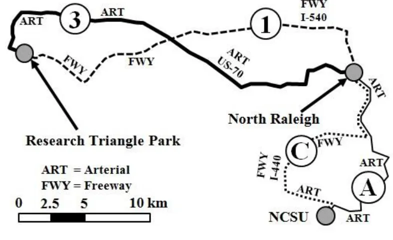
Scenarios, Traditional Single-family Detached House ... 65 Figure IV-1. Study Area Map ... 83 Figure IV-2. Comparison of PM2.5 Measurements between Two DustTrak DRX 8533

Monitors ... 85 Figure IV-3. Example Comparisons of Simultaneous Measurements for Near-Vehicle

and In-Vehicle PM2.5 Concentrations with Different Sources of Forced

Air, on Afternoons of June 29 for (a) and July 3 for (b) ... 88 Figure V-1. Study Area and Route Map in Raleigh, NC ... 105 Figure V-2. Example Comparison of Distance versus Concentration for Bus, Car, and

Pedestrian mode on Apr 3 Lunchtime, Outbound (Sections A and B) ... 112 Figure V-3. Distributions of the Ratios of Average PM2.5 Concentrations for Pairwise

Comparisons of Pedestrian-to-Car and Bus-to-Car by Time of Day and

Route Section ... 114 Figure V-4. Comparisons between Daily Average Near-Road Pedestrian PM2.5

1

2 1.1 Introduction

Particulate matter (PM) pollution is a mixture of microscopic solids and liquid droplets

suspended in the air. PM comes in a variety of sizes and can be made up of many types of

components, including acids (sulfates and nitrates), organic chemicals, metals, soil, or dust

particles, and allergens (fragments of pollen or mold spores) (U.S. EPA, 2013). Of particular

concern is a class of particles known as fine particulate matter (PM2.5) that is comprised of

particles 2.5 micrometers or smaller in aerodynamic diameter. They are small enough to

enter the lungs and cross the blood-air barrier in the alveoli. Based on review of numerous

studies, the U.S. Environmental Protection Agency (EPA) has identified causal associations

between exposure to PM2.5 and adverse human health effects including premature death in

people with heart or lung disease, nonfatal heart attacks, irregular heartbeat, aggravated

asthma, decreased lung function, and increased respiratory symptoms (U.S. EPA, 2009a).

People with heart or lung diseases, children, and older adults are the most vulnerable

subpopulations to be affected by particle pollution exposure (U.S. EPA, 2009a).

Exposure is defined as the contact of a chemical, physical, or biological agent with

the outer boundary of a human body (U.S. EPA, 1992). Exposure differs from internal dose,

which is the amount of a chemical absorbed upon crossing the boundary to biologically

significant sites within the body (U.S. EPA, 1992). While exposure can be conceptually

characterized as a linear function of concentration and time, the description of internal dose

is more complex because internal dose may depend on inter-individual variability in

physiological or other factors and is not usually just a simple linear function of concentration

3 A challenging aspect of air pollution health effects studies is to properly quantify the

exposures of individuals in the population. Ambient PM2.5 concentrations are affected by

meteorology and by changes in emission rates, and locations of emission sources. However,

actual PM2.5 exposure to ambient origin depends on the amount of time an individual spends

in different microenvironments. Microenvironments are surroundings that can be treated as

homogeneous or well characterized with respect to the concentrations of an agent (U.S. EPA,

1992). Microenvironments include various indoor locations (e.g. home, work, school,

restaurant, and store), outdoors, in transit, and others. For indoor microenvironments, a

portion of ambient PM2.5 penetrates and deposits to interior surfaces.

Exposure concentration is the concentration with which a person comes into contact

(U.S. EPA, 1992). An individual’s time-weighted PM2.5 exposure can be quantified as the

airborne PM2.5 exposure concentration integrated over a given time period based on the

person’s activities (U.S. EPA, 2009a):

E_T 



4 Figure I-1. Decomposition of Personal Exposure to PM

Previous studies generally found that individual daily values of total and non-ambient PM2.5 exposure were poorly correlated with the daily ambient concentrations, but the individual daily ambient exposures were highly correlated with ambient concentrations (U.S. EPA, 2004). Thus, the separation of total PM exposures into ambient and non-ambient components reduces potential uncertainties in the analysis and interpretation of PM health effects data (U.S. EPA, 2009a).

Ambient PM sources include industrial and mobile source emissions, re-suspended dust, biomass combustion, and secondary formation. Non-ambient sources include smoking, cooking, home heating, cleaning, and indoor air chemistry (U.S. EPA, 2009a). PM concentrations from both ambient and non-ambient origin subject to spatial and temporal variability, and can affect exposure and resulting health effect estimates. In addition, the chemical composition of PM2.5 can vary depending on the emission source, proximity to

Total Personal

Exposure (E

)

Ambient Exposure

(E

)

Ambient PM while

outdoors

Ambient PM that

infiltrates indoors

Non-ambient

Exposure (E

)

Indoor sources

(cooking, cleaning)

5 sources, or as a result of formation of secondary PM2.5. Furthermore, PM2.5 of different chemical compositions can have different size ranges and thus may penetrate differently from outdoors to indoors (U.S. EPA, 2009b).

Population exposure assessment will be useful in characterizing the relationship

between ambient concentration and population exposure, and the variability in population

exposures. Both of these are important to the interpretation of community time-series

epidemiological studies for establishing regulatory standards, such as the National Ambient

Air Quality Standards (NAAQS). In the last revision of the PM NAAQS, EPA did not

include an exposure assessment. This is in part because the health risks estimated using

ambient concentrations provided adequate information on the change in health risks

associated with a change in ambient concentrations, and a perception of the need for more

research to provide insights on population exposures to identify various personal and

building-related factors that may account for variability in PM2.5-associated health risks (U.S. EPA, 2009a).

6 The current NAAQS for PM2.5 were based on evidence of health effects associated with short- and long-term exposure to fine particles from epidemiologic studies, and ambient concentration is typically used as a surrogate for personal exposure (U.S. EPA, 2009a). However, in a four-city exposure study, average personal exposuresto ambient origin varied by individual, city and season, and were substantially less than the ambient concentrations

(Sarnat et al., 2009). Differences between personal ambient exposure and ambient concentration can result in the ordinal ranking of the mean concentrations and exposures in

each of the locations or seasons that are not the same, which can lead to biased health risk

estimates since the true relationships between exposure and response are not reflected in the

concentration-response (C-R) functions.

Since people spend majority of daily time indoors, on average for a population, the daily exposure to particles of ambient origin is typically less than the ambient concentration, and the difference contributes to exposure errors (Zeger et al., 2000). Using ambient PM2.5 concentrations as a surrogate for the community average personal exposure to ambient PM2.5 will negatively bias the estimation of health risk coefficients by the ratio of PM2.5 ambient exposure to ambient concentration (Ea/C) (Chang et al., 2012). These findings indicated how the selection of exposure metric can impact the risk estimates, and underscore the importance

of characterizing the Ea/C ratio to accurately estimate exposure to ambient PM.

7 to 1. Assessing inter-individual variability in Ea/C will acknowledge variability in exposures within a population, and help to identify high-end exposure subgroups.

U.S.-based multicity epidemiological studies generally found that PM2.5 effects differ

by season and region, with greater effects observed in eastern U.S. and during warmer months in spring and summer (U.S. EPA, 2009a). For example, Franklin et al. (2008) analyzed PM2.5 monitoring and daily mortality data in 25 cities nationwide between years 2000 to 2005, and reported a 80% higher effect estimate in the east (0.92% increase in non-accidental deaths associated with a 10 µg/m3 increase in 2-day averaged PM2.5 concentration) than in the west (0.51%). Spring showed the highest effect of 1.88% among all seasons, which was a factor of 11.5 higher than that of the lowest winter season (0.19%). An inverted U-shape curve was identified to illustrate the relationship between PM2.5 health effect estimates and seasonally-averaged ambient temperature (Franklin et al., 2008). Temperature was used as a surrogate for building ventilation, which varies by season and affects particle penetration to indoor microenvironments. When temperatures were moderate between 10 to 25°C, the estimated effects of non-accidental mortality were above the average effect, while effects were below average for both low and high temperatures.

8 season (2.01%) was about 2.7 times higher than for the summer (0.55%). Heterogeneity in PM2.5 health effects may result from seasonal and regional differences in emissions and

particle chemical constituents, and differences in exposure factors other than concentration,

including differences in home ventilation, indoor versus outdoor activity patterns, and

population demographics (Bell et al., 2008).

While Franklin et al. (2008) and Bell et al. (2008) used measured ambient PM concentration data for risk estimates, Chang et al. (2012) estimated the short-term effects of personal exposure to ambient PM2.5 in New York City for years 2001 to 2005 using two exposure metrics, including the fused Community Multiscale Air Quality model (CMAQ) data and the estimated exposure from an exposure simulator SHEDS-PM. Risk estimates associated with exposures were greater than that associated with concentrations, which indicated a negative bias in the concentration-response function when ambient levels were used as a proxy for exposure. The magnitude of the bias approximated the ratio between daily concentration and exposure level. When stratified by season, the risks of mortality associated with PM2.5 were higher and only statistically significant during the summer months. Such result agreed with previous seasonal analysis of PM10 and mortality in Northeastern US (Peng et al., 2005). This highlights the need to characterize geographic and seasonal variability in the Ea/C ratio on a population basis to aid in the interpretation of

epidemiologic findings.

There have been studies looking at the Ea/C ratio in exposure for pollutants such as

9

ratios for ozone are generally observed with increasing time spent outside and higher air

exchange rate. For CO, the average Ea/C ratios are around 1. For SO2, as a result of low

ambient SO2 concentrations and the limitations of passive sampling, only two studies have

reported average Ea/C ratios, with values ranging from 0.08 to 0.13. Differences in the Ea/C

ratio between pollutants are mainly related to pollutant-specific physical or chemical removal

processes. Ea/C ratios for ozone tend to be low because ozone is a highly reactive oxidant

that is removed from air by surface interactions and airborne constituents (U.S. EPA, 2013). In contrast, CO is relatively inert and has a much longer lifetime in air (U.S. EPA, 2010b). SO2 is highly soluble and thus can be removed by reactions on indoor surfaces, especially

those that are moist (U.S. EPA, 2008).

None of these characteristics applies to PM2.5. PM2.5 is not as chemically reactive as

ozone, as soluble as SO2, nor removed as slowly as CO. Thus, the Ea/C ratio for PM2.5 tends

to be substantially different than the Ea/C ratios for these other pollutants. The main removal

process for PM2.5 is deposition. Also, unlike the gaseous pollutants, the penetration efficiency

of PM2.5 from outdoors to indoor microenvironments is less than one, because of physical

processes such as impaction and interception (U.S. EPA, 2009a).

Due to the limitation of field studies, there is a need for research to develop modeling

approaches for exposure assessment. EPA has used the Air Pollution Exposure (APEX)

model for estimating human population exposure to ozone and CO, and produced substantial

information and data to support model development (U.S. EPA, 2013; U.S. EPA, 2010b). Although EPA recommended using APEX and/or the Stochastic Human Exposure and Dose

10

assessment (Glen et al., 2012; Burke and Vedamtham, 2009), there has not yet been a

systematic modeling analysis to quantify the Ea/C ratio for PM2.5 by region and season. A

goal of the study is to provide an example of the application of simulation-based exposure

modeling to quantification of variability in PM2.5 exposure, especially the Ea/C ratio.

Another important issue in PM epidemiological studies is to determine whether the C-R relationship is linear across the full concentration range or if there are concentration ranges that exhibit nonlinearity. Evidence suggests that the C-R relationship for PM2.5 is consistent with a linear no-threshold model at low levels (annual average concentrations from 5 to 30 µg/m3), but flattens out to be log-linear at higher long-term average concentrations on the order of 100 µg/m3 or more, such as for an active tobacco smoker or a person exposed to indoor solid-fuel combustion (Pope et al., 2009; Ezzati and Kammen, 2001). Therefore, it is important to accurately quantify non-ambient exposure from indoor emissions and assess the incremental health effect of PM2.5 from non-ambient exposure relative to a baseline of the relatively lower ambient exposure.

11 2002),indoor residential PM2.5 exposure has a substantial influence on total PM2.5 exposure. Based on a SHEDS-PM case study in Philadelphia, indoor residential exposure of ambient and non-ambient origins accounted for 28% and 42%, respectively, on total PM2.5 exposure of the population (Burke et al., 2001). However, ambient and non-ambient particles differ in sources and sizes, and likely to differ in composition and biologic properties as well (Abt et al., 2000; Long et al., 2001). Thus, characterizing the potential health impacts associated

with ambient and non-ambient particles within the indoor residence, separately, may help to reduce uncertainty in health risk estimates.

The current practice in stochastic population exposure models such as the Air Pollution Exposure (APEX) and Stochastic Human Exposure and Dose Simulation (SHEDS) typically assumes the home residence to be a single, well-mixed zone when calculating residential exposure. However, indoor emissions from cooking or smoking typically occur in a specific room, and the indoor mixing of PM2.5 from indoor emissions is mostly limited to that room initially. Therefore, the bias in non-ambient exposure concentration associated with the assumption of one large single zone within a home should be evaluated. In addition, there is a need to know how parameters such as air exchange rate, volume and type of the house, and emission rate and duration of non-ambient sources affect inter-individual variability in the distribution of indoor PM2.5 concentrations. Better quantification of dispersion of pollution within the indoor residential microenvironment is critical for PM2.5 exposure assessment.

12 indoors but the highest ambient PM2.5 exposure concentrations occur in on-road or near-road transportation microenvironments (U.S. EPA, 2009a). Typical personal transport in the U.S. include modes such as personal car, referred to as “in-vehicle,” transit bus and pedestrian walking, which comprise more than 90% of total trips (U.S. DOT, 2001). In the U.S., the average one-way daily commuting travel time is 25.5 minutes, and 86% of trips to work are via personal vehicle (McKenzie and Rapino, 2011). Depending on traffic flow, meteorological conditions, vehicle emission rates, whether windows are open, operation of the vehicle heating, ventilation, and air conditioning (HVAC) system, and time spent in-vehicle, in-vehicle exposure may account for 10 to 20 percent of total daily average PM2.5 exposure (Liu and Frey, 2011). The mode share of public transportation and pedestrian walking are comparably higher in large metro areas or areas with at least one large college or university that had high proportions of college-aged students (McKenzie and Rapino, 2011). A closer examination of PM concentrations on or near roadway is essential to accurately estimating individual exposure, and to identifying key factors affecting variability in exposures that may aid in developing improved exposure model estimates and effective control strategies.

1.2 Objectives

The objectives of this study are to:

13 (2) Improve PM2.5 exposure concentration estimates for the indoor residential

microenvironment; and

(3) Evaluate variability in PM2.5 exposure concentrations for the transportation microenvironments.

1.3 Organization

This dissertation consists of six parts. As an overview graph, Figure I-2 illustrates how parts of the dissertation are related with each research objective. Appendices are given at the end of the document. Each part of the dissertation contains a separate reference list.

Figure I-2. Overview of Research Scope Air Quality

Exposure (Part II)

Dose

Response

Microenvironmental Concentrations Time Spent in

Microenvironments Outdoors Indoors In-vehicle (Part IV and V)

Home (Part III)

14 Part I introduces the background information regarding PM2.5 exposure, as well as general exposure concepts, research motivation and objectives, and dissertation organization. Part II assesses inter-individual, geographic, and seasonal variability in estimated population exposure to PM2.5 using an exposure simulation model.

Part III develops a method to estimate correction factors for bias correcting the single-zone estimates of indoor residential PM2.5 concentrations to account for indoor emission sources such as cooking and smoking.

Part IV demonstrates a method for quantifying the ratio of in-vehicle to near-vehicle exposure concentrations of airborne PM2.5.

Part V compares PM2.5 concentrations in selected transportation modes including car, bus and walking, and identifies factors affecting in-transit exposure.

Part VI discusses and summarizes main conclusions of this research.

15

PART II ASSESSMENT OF INTER-INDIVIDUAL, GEOGRAPHIC, AND

SEASONAL VARIABILITY IN ESTIMATED HUMAN EXPOSURE TO FINE PARTICLES*

16 Abstract

17 2.1 Introduction

According to the U.S. Environmental Protection Agency (EPA) Integrated Science Assessment (ISA) for Particulate Matter, a causal or likely to be causal relationship exists between short-term (daily) human exposure to fine particulate matter (PM2.5) and several health effects, such as mortality, cardiovascular and respiratory morbidity (U.S. EPA, 2009a). Children and adults 65 years and older are the two most susceptible subpopulations (U.S. EPA, 2009a). The proportion of older adults in the US population will increase from 13% in 2011 to 20% in 2030 (U.S. Census Bureau, 2000). Thus, PM-related health incidents could occur more frequently in the future.

18 than the ambient concentration, and the difference contributes to exposure error (Carroll et al., 1995; Zeger et al., 2000). Using ambient PM2.5 concentrations as a surrogate for the community average personal exposure to ambient PM2.5 will bias the estimation of health risk coefficients by the ratio of ambient PM2.5 exposure to ambient PM2.5 concentration (Ea/C) (U.S. EPA, 2009a).

Findings from PM2.5 exposure panel studies indicate substantial variability in 24-h average personal PM2.5 exposures among US regions (Wallace and Williams, 2005; Williams et al., 2003; Weisel et al., 2005; Sarnat et al., 2005). Individuals are exposed to PM2.5 of both

ambient and nonambient origin, and both sources of PM2.5 may contribute to adverse health outcomes. Total and nonambient PM exposure are poorly correlated with ambient PM concentration (Wilson et al., 2000).Ambient PM concentrations are affected by meteorology and by changes in emission rates and locations of emission sources, whereas nonambient PM concentrations are influenced by daily activities of people. The Ea/C ratio depends on housing type and activity patterns, air exchange rate, and PM deposition rate. It varies between 0 and 1 among individuals, and varies among cities and seasons (Sarnat et al., 2007). Since concentration-response functions are typically heterogeneous across cities and seasons, characterizing the factors that influence Ea/C could be useful in correcting for exposure error.

19 to more than a month before the date of death (Schwartz, 2000). Thus, averaging times other than 24-hr averages should be considered to provide appropriate modeling results for sub-acute or chronic health effects applications (Özkaynak et al., 2009). Therefore, quantification of the sensitivity of inter-individual variability in exposure with respect to different averaging times may help to better inform health effects studies.

PM2.5 exposure can be estimated based on field study or simulation models. Measured exposure data mainly come from either a few multi-city probability-based field studies, such as the Relationship between Indoor, Outdoor and Personal Air (RIOPA) study, the Detroit Exposure Aerosol Research Study (DEARS), and the Canadian Windsor Ontario Exposure Assessment Study (WOEAS), or longitudinal panel studies focused on small numbers of exposed individuals in susceptible subpopulations, such as the elderly (Weisel et al., 2005; Williams et al., 2009; Wheeler et al., 2011; Williams et al., 2000).

20

As summarized by Sarnat et al. (2007), several measurement studies have been

conducted to estimate the associations between PM2.5 personal ambient exposure and

ambient concentration, which can be used to estimate the Ea/C ratio. Although there have

been studies that quantified geographic and seasonal variability in the Ea/C ratio for other

pollutants, such as ozone, CO, and SO2, there has not been systematic quantification of

variation in for PM2.5 using a consistent framework (U.S. EPA, 2012; U.S. EPA, 2010b; U.S.

EPA, 2008). Ea/C ratios differ substantially among pollutants depending on chemical

reactivity, solubility, and pollutant lifetime. The average Ea/C ratios for highly reactive ozone

are typically 0.1 to 0.3, for relatively unreactive CO are around 1, and for highly soluble SO2

are from 0.08 to 0.13. In contrast, the Ea/C ratio for PM2.5 depends on factors such as

interception and impaction that affect penetration from outdoors to indoors, and indoor

deposition rate (U.S. EPA, 2009a).

The objectives of this paper are to: (1) assess the sensitivity of inter-individual variability in exposures with respect to averaging time; (2) evaluate geographic differences in individual variability in exposures; and (3) evaluate seasonal differences in inter-individual variability in exposures.

2.2 Methodology

The methodology includes: (1) scenario-based exposure modeling; (2) study design and

21 2.2.1 Scenario-based Exposure Modeling

Burke et al.(2001) evaluated SHEDS-PM using measurement data from a PM panel study conducted in the Research Triangle Park, NC area. The model predictions of individual and population exposures to PM2.5 are generally consistent with the estimates derived from the personal measurement data. Other studies have reviewed the algorithms and input data for SHEDS-PM, and recommended improvements are incorporated here. Cao and Frey reviewed default Environmental Tobacco Smoke (ETS) related inputs and recommended updates to input data for the proportion of smokers and other smokers, and for cigarette emission rates (Cao and Frey, 2011a). Liu et al. reviewed the algorithms and default inputs for the in-vehicle microenvironment, and proposed an alternative approach which integrates a dispersion model and a mass balance approach (Liu et al., 2010).Cao and Frey recommended updates to the distributions of ACH, P, and k for selected areas and seasons (Cao and Frey, 2011b).

22 sources. Simulated microenvironments include outdoors, home, office, school, store, restaurant, bar and vehicle.

For the residential microenvironment, SHEDS-PM utilizes a single-compartment, steady state mass balance equation to calculate residential PM2.5 concentration (Burke and Vedamtham, 2009). The contribution from indoor emission sources such as smoking, cooking, cleaning and other sources is quantified. The housing type categories in

SHEDS-PM are single-family detached, single-family attached, multiple family, mobile home and

other. Based on the US Census 2000 Housing Survey, lognormal distributions are used for

23 2.2.2 Study Design

The focus here is to quantify possible regional and seasonal variability in estimated exposure. Adults over 65 years old are selected because they are a susceptible subpopulation with respect to PM2.5 exposure (U.S. EPA, 2009a). To address regional differences, three urban areas are chosen to represent diverse southeast, south central and northeast US climate zones. These areas include: (1) a six-county area in North Carolina along Interstate 40, comprised of Wake, Durham, Orange, Alamance, Guilford, and Forsyth Counties, that includes the cities of Raleigh, Durham, Burlington, Greensboro, High Point, and Winston-Salem; (2) Harris County in Texas, including the city of Houston; and (3) New York City, including Bronx, New York, Kings, Queens, and Richmond Counties. Approximately 50,000 individuals 65 years and older are simulated from all census tracts of each area for a period of 30 days in each season. To address seasonal differences, one month from each of four seasons is selected, including April for spring; July for summer; October for fall; and December for winter. SHEDS-PM model version 3.7 was used to run all cases. Typically it takes approximately 5 to 6 hours of CPU time to simulate exposures for 50,000 individuals for a 30-day time period.

24 ETS is modeled in residential, restaurant, and bar microenvironments. The proportions of smokers and non-smokers are estimated based on region-specific 2002 data (State Center for Health Statistics, 2002; Marshall et al., 2006; U.S. DHHS, 2006; NYC Department of Health and Mental Hygiene, 2002). Input parameters for residential microenvironments, such as ACH, P, k, and cigarette emission rate, and for the in-vehicle microenvironment, are specified based on related literature (Cao and Frey, 2011a; Liu et al., 2010; Cao and Frey, 2011b; Özkaynak et al., 1996; Murray and Burmaster, 1995; Koontz and Rector, 1995). Parameters of other microenvironments are based on Burke et al.(2001).

2.2.3 Statistical Analysis Methods

SHEDS-PM outputs are processed and analyzed using Predictive Analytics SoftWare (PASW) 18.0. The SHEDS-PM model quantifies time spent by each simulated individual in different microenvironments and the corresponding microenvironmental PM2.5 concentrations, and estimates daily average Ea, Ena, and Et for each simulated individual. The Ea/C ratio is calculated for each simulated individual for each simulated day.

25 To examine the sensitivity of inter-individual variability with respect to averaging time, the daily Ea/C ratio is further averaged by individual over one month to represent a longer term. Both daily and monthly ratios of Ea/C are compared for each geographic area and season. The analysis included comparisons of 95% frequency ranges inferred from simulated cumulative distribution functions (CDFs) of inter-individual variability in exposure, and comparisons of the effect of longitudinal versus randomized day-to-day sampling of activity dairies on the distribution of monthly average exposures. Individual daily exposure values are extracted from SHEDS-PM output to construct a 50,000 individual by 30 day

exposure matrix. For each day, correlations of inter-individual variability in exposure are

calculated with each other day. Days are categorized by day type, including weekday,

Saturday and Sunday. For each of the 30 days, the average correlation with all other days of

the same type, and with all days of each of the other two types, are estimated.

To assess the geographic and seasonal differences in inter-individual variability in exposures, daily ratios of Ea/C, Ena and Et are compared among geographic areas for the same season and among multiple seasons for the same area.

2.3 Results 2.3.1 Key Inputs

26 Values of ACH, P, and k for the residential microenvironment are shown in Table

II-1. Distributions of variability in ACH by geographic region are based on the Relationship of

Indoor, Outdoor and Personal Air (RIOPA) study(Weisel et al., 2005) from 1999 to 2001, Murray and Burmaster (1995), Koontz and Rector (1995), and Wallace et al. (2006).

Distributions of variability in P and k are based on the PTEAM and RIOPA studies

(Özkaynak et al., 1996; Weisel et al., 2005). The distribution types are selected based on Cao

and Frey(2011b) and are explained in the Appendix A. Sensitivity analysis by Cao and Frey

(2011b) assessed the effects of ACH, P and k on estimated human exposures. ACH is the

most sensitive input for both ambient and non-ambient exposure to PM2.5, whereas the results

are not sensitive to the choice of distribution for P and k.

Table II-2 shows other input factors that affect inter-individual exposure variability,

such as demographics, smoking prevalence, housing types, and human activity patterns.

Females account for approximately 60 percent of the total elderly population in each area.

Exposure to indoor sources of PM2.5 is typically higher as the housing interior volume

decreases (Cao and Frey, 2011b). The population weighted average time spent in different

27 Table II-1. Residential Microenvironment Input Parameters

Parameter Distribution Type a

Location b Season Value c Penetration

(P)

Triangular ALL ALL Min= 0.70, Mode= 0.78,

Max= 1.0

Deposition (k) Normal ALL ALL µ = 0.40 h-1, σ = 0.01 h-1

Air Exchange Rate (ACH)

Lognormal

NC domain

Winter µg = 0.38 h-1, σg = 1.80 h-1 Spring µg = 0.31 h-1, σg = 2.31 h-1 Summer µg = 0.54 h-1, σg = 1.70 h-1 Fall µg = 0.49 h-1, σg = 1.62 h-1 Harris County,

TX

Winter µg = 0.56 h-1, σg = 2.20 h-1 Spring µg = 0.38 h-1, σg = 1.80 h-1 Summer µg = 0.37 h-1, σg = 1.90 h-1 Fall µg = 0.65 h-1, σg = 1.80 h-1 NYC

Winter µg = 0.45 h-1, σg = 2.03 h-1 Spring µg = 0.40 h-1, σg = 1.82 h-1 Summer µg = 0.64 h-1, σg = 2.09 h-1 Fall µg = 0.22 h-1, σg = 1.72 h-1 a.

Triangular distribution parameters are the minimum, mode, and maximum; normal distribution parameters are the mean µ and standard deviation σ; lognormal distribution parameters are the geometric mean µg and standard deviation σg. The selection of distribution types are based on Cao and Frey (2011) and is described in the Appendix A. b.

NC includes Wake, Durham, Orange, Alamance, Guilford, and Forsyth Counties; TX includes Harris County; NYC includes Bronx, New York, Kings, Queens, and Richmond Counties.

c.

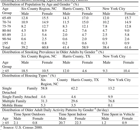
28 Table II-2. Exposure Model Demographic Input Data Regarding Population Distribution, Smoking Prevalence, Housing Types, and Activity Patterns

Distribution of Population by Age and Gender a (%) Age

Group

Six-County Region, NC Harris County, TX New York City

Male Female Male Female Male Female

65-69 12.8 15.5 14.3 17.0 12.0 15.7

70-74 10.9 14.9 11.5 15.0 10.2 14.9

75-79 8.2 12.7 8.3 12.1 7.8 12.8

80-84 4.5 8.9 4.2 7.6 4.7 9.0

85-89 2.1 5.6 2.0 4.7 2.5 5.8

90-94 0.6 2.5 0.6 2.0 0.9 2.6

≥95 0.2 0.8 0.2 0.6 0.3 0.9

Total 39.2 60.8 41.4 58.9 38.4 61.6

Distribution of Smoking Prevalence in Older Adults by Gender b (%)

Six County Region, NC Harris County, TX New York City Age

Group

Male Female Male Female Male Female

≥ 65 18.5 10.5 12.0 4.6 9.3 10.4

Distribution of Housing Types c (%)

Six County

Region, NC

Harris County, TX New York City

Single Family

Detached

58.8 62.2 13.2

Single Family Attached 4.6 4.6 9.9

Multiple Family 31.3 29.6 76.8

Mobile Home 5.3 3.5 0.1

Distribution of Older Adult Daily Activity Patterns by Gender d (hr/day) Age

Time Spent Outdoors Time Spent Indoor Time Spent in Vehicle

Male Female Male Female Male Female

≥ 65 2.1 0.8 20.7 22.3 1.2 0.9

a.

Source: U.S. Census 2000. b.

Sources: NC and TX – Behavioral Risk Factor Surveillance System (BRFSS), 2002; NYC – Epiquery, 2002.

c.

Source: U.S. Census 2000 – Housing Survey. Average indoor volume: single family detached: 466 m3; single family attached: 371 m3; multiple family: 241 m3; mobile home: 222 m3.

d.

29 2.3.2 Output

Inter-individual variability in estimated exposure to PM2.5 is compared with respect to

averaging time, area, and season.

Averaging Time

Inter- and intra-individual variability in exposure are compared based on the CV of inter- and intra-individual variability in daily exposure, respectively, as detailed in Table A-3 of the Appendix A. Inter-individual variability results in part from spatial variation in ambient concentration. However, inter-individual variability is also influenced by other factors such as ACH and activity. For the NC spring case, on average, CVs of inter- and intra-individual variability in daily average C are 0.11 and 0.32, respectively. Thus, C varies relatively little over space and among exposed individuals on a given day, and varies more substantially with time from day-to-day, which is consistent with other studies that are summarized in the PM ISA (U.S. EPA, 2009a). However, inter-individual variability in exposure is influenced by variability in other factors in addition to C. The CV of inter-individual variability in Ea is 0.37, which is much larger than that for C. The CV of intra-individual variability in Ea is 0.45, which is 18% higher than for inter-individual variability. Thus, exposure varies more over time than it does between individuals on a given day. The CV of Ea/C is similar (about 0.3) for both inter- and intra-individual variability, indicating that factors influencing Ea other than C, such as ACH, P, and k have similar variability among individuals or over time.

30 in estimated Ea/C for each geographic area and season, they have the same mean as expected, but the standard deviation of the daily average Ea/C is approximately twice that of the monthly average. The 95% frequency interval for the daily average Ea/C ratio typically ranges from 0.2 to 0.9, whereas the range for the monthly average is approximately 0.3 to 0.7, as shown in Figure II-1 for the NC domain in spring. The variation in Ea/C is reduced as the averaging time increases, since day-to-day variations are averaged out for each individual. For the NC spring case, the correlations of inter-individual variability in daily Ea/C among days of the same day type are around 0.4, whereas there is little correlation among days of different day types.

Figure II-1. Comparison of Inter-Individual Variability in the Ratio of Estimated Ambient Exposure to Ambient Concentration (Ea/C) for Selected Averaging Times, NC domain, Spring 2002

The range of the distribution of monthly average Ea/C is influenced in part by the method used in SHEDS-PM for longitudinal sampling of activity diaries. To explore how

0.0 0.2 0.4 0.6 0.8 1.0

0.0 0.1 0.2 0.3 0.4 0.5 0.6 0.7 0.8 0.9 1.0

Cum

u

lative

F

re

q

u

en

cy

31 sensitive the results are to this sampling method, an alternative NC spring case was analyzed in which individuals were randomly sorted from day-to-day, thus leading to no significant correlation in day-to-day comparisons of inter-individual variability. Because the longitudinal simulation is based on positive correlations from day-to-day, it is expected to provide a wider range of monthly average inter-individual variability than a randomized simulation. The difference in results between the two cases indicates whether longitudinal simulation has a significant effect. For the randomized case, the 95% frequency range in inter-individual variability of monthly average Ea/C is from 0.43 to 0.55, which is about one-third the range of the longitudinal case. Thus, the results are sensitive to the approach used for longitudinal simulation.

Geographic Variability

32 Table II-3. Geographic and Seasonal Variability in Exposure a

a.

Mean and standard deviation are based on individual daily average exposures obtained using the Stochastic Human Exposure and Dose Simulation for Particulate Matter (SHEDS-PM).

b.

NC includes Wake, Durham, Orange, Alamance, Guilford, and Forsyth Counties; TX includes Harris County; NYC includes Bronx, New York, Kings, Queens, and Richmond Counties.

c.

Ea/C: ratio of ambient exposure to ambient concentration; Ea: ambient exposure (µg/m3); Ena: non-ambient exposure (µg/m3); Et: total exposure (µg/m3).

2012), which leads to lower air exchange and consequently lower Ea/C ratio than NC and NYC.

33 (a) Six-County Area, North Carolina

(b)Harris County, Texas

(c) New York City

Figure II-2. Geographic and Seasonal Variability in the Ratio of Estimated Daily Ambient Exposure to Ambient Concentration for the NC domain, Harris County, and NYC, 2002

0.0 0.2 0.4 0.6 0.8 1.0

0 0.1 0.2 0.3 0.4 0.5 0.6 0.7 0.8 0.9 1

C umul at ive F re q u en cy

Ratio of Ambient Exposure to Ambient Concentration (E_a/C) winter spring summer fall 0.0 0.2 0.4 0.6 0.8 1.0

0 0.1 0.2 0.3 0.4 0.5 0.6 0.7 0.8 0.9 1

Cum u lative F re qu ency

Ratio of Ambient Exposure to Ambient Concentration (E_a/C) winter spring summer fall 0.0 0.2 0.4 0.6 0.8 1.0

0 0.1 0.2 0.3 0.4 0.5 0.6 0.7 0.8 0.9 1

Cum u lative F re q u en cy

34 Generally, Ena is most sensitive to ACH. Areas with lower ACH tend to have higher average Ena. However, the combined effect of lower smoking prevalence and higher indoor housing volume sometimes can be more influential than ACH, as illustrated by the TX domain in summer. This domain has the smallest proportion of smokers and largest average indoor volume. Although the summer ACH is much less for the TX versus NC or NYC domains, the population average Ena for the TX domain is the lowest.

The daily average Et varies by 10% to 28% among geographic areas for any given season for the total population. However, non-smokers not exposed to ETS have much lower average Et than persons with ETS exposure. For people with ETS exposure, approximately 85% of daily Et is non-ambient. Thus for those with ETS exposure, the average Et is highly influenced by the non-ambient exposure level. This is because the upper-tail values of Ena (above the 90th percentile) are usually 2 to 10 times higher than for Ea.

Seasonal Variability

In the same region, the average daily Ea/C ratio differs among seasons by 16% in the NC domain and by 34% in NYC, as shown in Table II-3. Many dwellings in NYC are not air conditioned, and residents tend to open windows more in the summer. In contrast, in Harris County, the average Ea/C is 15% lower in summer than in the fall. For the NC domain, the Ea/C ratios are similar between summer and fall. The seasonal difference in the Ea/C ratio is partly associated with more widespread air conditioner use in TX and NC (U.S. EPA, 2012).

35 prevalence, indoor volume, demographics, and individual activity patterns, seasonal differences in Ena are most sensitive to seasonal differences in ACH.

The seasonal variability in estimated average daily Et is not as pronounced compared to geographic variability. The difference in the average daily Et among seasons for a given region ranges from 15% to 19%, which is mainly attributed to seasonal variations in ACH. For people exposed to ETS, because Et is dominated by the contribution of non-ambient exposure, higher ACH leads to lower Et. But for non-smokers, Ena only accounts for about 40% in their daily Et on average. Therefore, higher ACH leads to higher Et for non-smokers.

2.4 Discussion and Conclusions

As expected, the ambient air quality data in grid cells used as input to the SHEDS-PM model typically exhibited rather low spatial variation within a geographic domain on each day, with CV < 0.2 for 11 of the 12 area and season cases studied. Daily average ambient exposures are significantly lower than ambient concentrations and vary by season and location. Furthermore, there is substantial inter-individual variability in exposure that is not explained by ambient concentration alone.

36 pattern by gender, region, and season for the specific geographic areas that are the focus here. Clearly, there is a need to further develop CHAD to contain diaries representative of geographic areas and seasons of interest, and to refine the exposure model to take ambient conditions into account when sampling diaries.

The CV in time spent outdoors among individuals was found to be similar to the CV for 11 individuals for whom more than 4 days of diaries were available in CHAD. Thus, the limited evidence suggests that activity patterns are repeatable from day-to-day and similar among individuals, at least for the selected subpopulation. The simulation model appropriately accounts for similarity in day-to-day activity.

Non-ambient exposure to PM2.5 is approximately uncorrelated with ambient concentration (average rp = -0.002, as detailed in Table A-6 of the Appendix A), which is consistent with other studies that are summarized by EPA(U.S. EPA, 2009a). Average levels of Ena vary by area and season mainly because of differences in ACH. For people exposed to ETS, Ena is the dominant contributor to Et.

37 the use of ambient concentration as a surrogate for ambient exposure in epidemiology studies may still account for temporal trends in exposure.

The distribution of Ea/C ratios in each area and season implies that, in general, exposure to ambient PM2.5 is less than the ambient concentration. On average, exposures to simulated individuals are approximately half of the ambient concentrations. These findings indicate that concentration-response functions developed in epidemiological studies using ambient concentration as surrogate for exposure are biased when compared to exposure concentration.

Exposure, and not just concentration, should be considered in developing risk management strategies to reduce uncertainty in health effect estimates, and to identify highly exposed groups and possible exposure reduction strategies. High-end daily average ambient exposures among individuals are influenced by factors other than high ambient concentration, such as ACH by location and season. ACH is related to housing type and ventilation practices used. Ea/C is well correlated (rp=0.5 to 0.6) with ACH, but has little correlation with ambient concentration C. Thus the distribution of inter-individual variability in the Ea/C ratio can be used to identify the need for providing advisory information to the public. Such information might include, for example, advice to reduce ventilation with outside air on high ambient PM2.5 days.

38 Ea/C ratio. The range in mean Ea/C among studied areas and seasons is from 0.44 to 0.60. The difference between these ratios is statistically significant based on the simulated results and represents a 36 percent relative difference. Because Ea/C ≥ 0 and typically Ea/C < 1 for most individuals, the population mean of Ea/C is constrained and therefore the range of possible difference in average Ea/C ratio is also constrained. Region and season-specific Ea/C ratios are recommended as a factor to consider when interpreting heterogeneity in epidemiologic studies.

2.5 Acknowledgements

39

PART III METHOD FOR BIAS CORRECTION OF ESTIMATED INDOOR

40 Abstract

41 3.1 Introduction

Epidemiologic studies have demonstrated a positive relationship between ambient fine particulate matter (PM2.5) concentration and adverse health effects, such as cardiovascular and respiratory morbidity and mortality (U.S. EPA, 2009a).Individual exposures to PM2.5 occur both outdoors and indoors. Indoor PM2.5 concentrations are affected by the penetration of ambient PM2.5, which leads to ambient exposure that takes place indoors; and non-ambient sources such as cooking and smoking, which leads to non-ambient exposure (Wilson et al., 2000). Since people spend at least half of their time per day in their residence (Stallings et al., 2002), indoor residential PM2.5 exposure has a substantial influence on total PM2.5 exposure. Therefore, quantification of dispersion of pollution within the indoor residential microenvironment is critical for PM2.5 exposure assessment.

3.1.1 Scope

42 Various modeling tools are available to estimate human exposure to PM2.5, including the Air Pollutant Exposure Model (APEX)(Glen et al., 2012) and the Stochastic Human Exposure and Dose Simulation Model for Particulate Matter (SHEDS-PM) (Burke and Vedamtham, 2009). SHEDS-PM is selected because it has previously undergone evaluation and has been applied in recent assessment of PM2.5 exposure (Burke et al., 2001; Cao and Frey, 2011a; Cao and Frey, 2011b; Jiao et al., 2012).

Key SHEDS-PM inputs include human activity data from the Consolidated Human Activity Database (CHAD), demographic and housing type data from the US Census, air quality data and microenvironment-specific inputs (Burke and Vedamtham, 2009). For the indoor residential microenvironment, SHEDS-PM uses a single-compartment, steady-state mass-balance equation to predict indoor PM2.5 concentrations (Burke and Vedamtham, 2009). Air exchange rate (ACH), indoor residential volume, deposition factor and penetrate rate are factors that affect the infiltration of ambient PM2.5 and the dilution of non-ambient PM2.5:





smk cig cook cook

r a

E N E t

P ACH

C C

ACH k ACH k VT

 

 

_{ } 

 

  (3-1) Where,

Cr = indoor residential PM2.5 concentration (μg/m3) Ca = ambient outdoor PM2.5 concentration (μg/m3) P = penetration factor (unitless)

43 V = residential volume (m3)

T = model time step

Esmk = emissions rate for cigarette smoking (mg/cig) Ncig = number of cigarette smoked during model step time Ecook = emission rate for cooking (mg/min)

tcook = time spent cooking during model time step (min)

The first term in Equation (3-1) describes the amount of outdoor PM2.5 that infiltrates into the residential microenvironment. The second term describes the PM2.5 generated from indoor sources. Equation (3-1) can be extended to include additional indoor sources such as use of cleaning products.

44 kitchen and the adjacent zones (Cao and Frey, 2011a). Indoor residential smoking is also a potential key source of indoor PM2.5 (Klepeis and Nazaroff, 2006). Therefore, the comparison should be carried out based on room-specific emissions from cooking and smoking.

Because the data needs and modeling requirements for simulating multiple zones are significant, it is not practical to implement a multi-zone model directly in SHEDS-PM. Instead, the development of a correction factor may enable a bias correction from the single-zone indoor PM2.5 concentration estimates. A correction factor is the ratio of time-weighted average PM2.5 concentration in the multi-zone versus single-zone approach.

3.1.2 Objectives

The objectives of this work are to:

(1) Compare indoor residential multi-zone and single-zone modeling approaches; (2) Develop a bias correction factor to infer indoor exposure concentration from a

single-zone simulation;

(3) Assess the sensitivity of correction factor with respect to variation in key inputs; and

(4) Demonstrate the implementation of correction factor.

3.2 Methodology

45 to the single-zone estimation; (4) conduct sensitivity analysis using the indoor air quality model to assess the impact of input variation on the correction factor; (4) implement the correction factors with SHEDS-PM; and (5) conduct bounding case analyses to demonstrate the sensitivity of exposure estimates to bias correction.

3.2.1 Mass Balance Inputs

Based on Equation (3-1), the fraction of outdoor PM2.5 that infiltrates indoors depends on ACH, k, and P. In addition, parameters such as indoor volume, emission rate and duration from indoor emission sources such as cooking and smoking are critical in estimating indoor residential PM2.5 concentration from indoor emissions.

46 which to estimate k and P (Cao and Frey, 2011b). The default values of k and P in SHEDS-PM were obtained from the Particle Total Exposure Assessment Methodology (PTEAM) study conducted for Riverside, California, in the fall of 1990 (Özkaynak et al., 1996).

Cao and Frey(2011b) recommended distributions of ACH, P and k based on results of literature review and sensitivity analysis. Data regarding ACH were reviewed mainly based on Murray and Burmaster (1995) and the Relationship of Indoor, Outdoor and Personal Air (RIOPA) study from 1999 to 2001 (Weisel et al., 2005). Data regarding P and k were reviewed mainly based on the RIOPA (Özkaynak et al., 1996) and PTEAM(Weisel et al., 2005) studies. ACH is distinguishably the most sensitive input for both ambient and non-ambient PM2.5 exposure, whereas exposures are relatively insensitive to variations in k and P (Cao and Frey, 2011b).

SHEDS-PM has default values for average indoor residential volumes of different housing stocks in US. These volumes are based on the US Census 2000 Housing Survey (U.S. Department of Commerce, 2013). Typical housing types include single-family detached house, single-family attached house, multi-family apartment, and mobile home.

48 Table III-1. Distribution of Individual Daily Time Spent in Consolidated Human Activity Database (CHAD)a

Information Reported by Microenvironment Number of Diaries in CHAD Mean (hr/day) Median (hr/day) Standard Deviation (hr/day) Home: diaries have any

location information (specificb or generalc)

21455 16.3 16.0 4.6

Home: diaries have both specific and general location information

9946 17.1 17.0 4.3

Home: diaries have only specific location information

7515 15.2 14.8 4.8

Home: diaries have only general information

3994 16.4 16.0 4.4

Home: diaries have activity in

kitchen 14208 1.4 1.0 1.3

Home: diaries have activity in

living room 14297 3.7 2.9 3.1

Home: diaries have activity in

bedroom 17196 10.0 10.0 3.0

Home: diaries have activity in

other specific rooms 11995 1.1 0.5 1.6

All outdoors ₁₃₄₇₀ 2.5 1.5 2.7

All in-vehicle ₁₈₂₉₅ 1.5 1.1 1.6

Other indoors ₁₇₉₄₅ 6.1 6.0 4.1

a.

The current version of CHAD in SHEDS-PM model contains 21,667 diaries in total. Each diary contains multiple locations information that the individual spent time in, including indoors, outdoors and in-vehicle microenvironments.

b.

“Specific” means the diary indicates the specific home location that the individual spent time in, such as kitchen, living/family room, bedroom, dining room, bathroom, study/office, basement, and utility/laundry room.

c.

“General” means the diary uses location codes such as “residence, general” (code = 30000), “your residence” (code = 30010), “residence, indoor” (code = 30020), and “your residence, indoor” (code = 30120) to indicate the individual’s location at home.

3.2.2 Indoor Air Quality Model

49 emission scenarios and work with either single- or multi-zone approach should be selected. A number of multi-zone airflow models have been developed during the past three decades and have been reviewed and evaluated (Feustel and Dieris, 1992; Emmerich, 2001; Sparks et al., 1991). Examples of such models are CONTAM (Dols et al., 2000), COMIS (Feustel, 1999), and RISK (Sparks, 2005). These multi-zone models use similar equations for predicting indoor air, and are able to simulate both mechanical and natural ventilation in the ventilation system.

RISK model

The RISK IAQ model incorporates results from EPA research on sources, sinks, ventilation, and air cleaners on indoor air quality (Sparks, 2005). RISK can estimate indoor concentrations based on indoor emission sources. Therefore, RISK was used to compare estimated PM2.5 concentrations between single- and multi-zone approaches under different emission scenarios.

50 Computational study design

To compare the estimated indoor PM2.5 concentrations between single and multi-zone approaches, two modeling cases were formulated in RISK for a typical floor plan of each of the four housing types included in SHEDS-PM and for indoor source emissions scenarios for cooking and smoking. The average single-zone volume used for each housing type in SHEDS-PM equals the average volume of each categorized housing type from the US Census 2000 Housing Survey (U.S. Department of Commerce, 2013). Persily et al. (2008) identified a collection of about 200 homes representing 80% of the US housing stock based on two residential housing surveys, the US Department of Energy Residential Energy Consumptions Survey (RECS) and the US Census American Housing Survey (AHS). For each housing type, the floor plan from Persily et al. (2008) with indoor volume approximately equal to the average volume from AHS was selected. Multi-zone characteristics regarding the number and volume of rooms were inferred from each selected floor plan. The sum of the volume of all rooms equals the volume used for the single-zone.