STUDENT COPULA METHOD IN RAINFALL DISTRIBUTION
Sharainie binti Sahrin, PM.Dr.Fadhilah Yusof
1.1 INTRODUCTION
Copulas are tools for modelling dependence of several random variables. The term copula was first used in the work of Sklar (1959) and is derived from the latin word copulare, to connect or to join. The main purpose of copulas is to describe the interrelation of several random variables. (Thorsten Schmidt, 2006).
Copula is a function that joins the two distributions and known as dependence functions. Copula connect multivariate distribution function to its univariate marginal distribution. When we have two models having the problems relating to dependence, we can join that models becoming one model using marginal function. So, the dependency is taken care. It means that copula played an important role to join multivariate distributions to their one dimensional marginal distribution function.
1.2 PROBLEM STATEMENT
This study will focus on expressing the bivariate distribution function from two univariate distribution functions. Considering these two distribution functions are independent, the multiplication of these two distributions can be done. However, in this case, the dependency between these two distributions must be considered. One of the way allowing the dependency of these distributions by using copula method.
1.3 LITERATURE REVIEW
The Word Copula is a Latin noun that means ''A link, tie, bond''. In 1959, the word Copula appeared for the first time.
Copula played an important role to join multivariate distributions to their one dimensional marginal distribution function. When we are having the problems relating to dependence, we can join that models becoming one model using marginal function as we want dependency is taken care.
Copula method has been used for flood frequency analysis. This analysis was based on t -copula for Johor River, Malaysia. Student Copula was used to model the joint dependence of peak flow-volume, volume-duration and peak flow-duration. (Salarpour et al., 2013).
Copula also has been used to model bivariate rainfall distribution. This model has been simulated at two sites in the Murray-Darling Basin, Australia. The selected sites are Hume and Beechworth. In this study, the asymmetric t-copula, also known as skew-t is used to analyse the monthly rainfall data.(Zakariaet al., 2010)
1.4 METHODOLOGY
If Y1and Y2 are jointly continuous random variables with a joint density function given by f(y1,y2), then
1. f(y1,y2) ≥0 for all y1, y2 2.
( 1, 2) 1 2 1
dy dy y y f
Joint distribution function is:
] , [ ) ,
(x y P X x Y y
H (1.1)
Marginal distribution function: ] [ ) ( ], [
)
(x P X x G y PY y
F (1.2)
Gamma Distribution
The PDF an d CDF of the gamma distribution with continuous shape parameter (), continuous scale parameter (
) and continuous location parameter (
) are as depicted below:)
/
)
(
(
exp
)
(
)
(
)
(
1
x
x
x
f
(1.3)
)
(
)
(
)
(
( )/
xx
F
(1.4) Where:
x
Parameter Estimation: Likelihood function
ni i n
i n n
i i
x
x
L
1 1
1
1
exp
)
(
)
(
(1.5)
The log-likelihood function iS
ni
n
i
i i
x
n
n
x
1 1
)
(
ln
ln
)
(
ln
)
1
(
(1.6)
n
i
i n n
x l
1
0 ) ( ln
) (
ln
(1.8)
0
)
(
)
1
(
1 1
n
x
l
n i i (1.9) Use Newton-Raphson method.
)
(
)
(
)
(
3 2 1 1 1 1 1
f
f
f
J
i k k k k k k k (1.10) 2 2 2 2 2 2 2 2 2 2 2 2 3 3 3 2 2 2 1 1 1 ln ln ln ln ln ln ln ln ln ) ( ) ( ) ( ) ( ) ( ) ( ) ( ) ( ) (
L L L L L L L L L f f f f f f f f f J i k (1.11) Weibull DistributionThe PDF and CDF of the weibull distribution with continuous shape parameter (), continuous scale parameter (
) and continuous location parameter (
) are as depicted below:
x
x
x
f
(
)
exp
1 (1.12)
-x
-exp
1
)
(
x
F
(1.13)Where:
x
Taking the logarithm for the likelihood function will get the log-likelihood function:
n i n i n i n i n i i i i x x x n n X l1 1 1 1 1
ln ln ) ln( ) ln( ln ln ) ; , , ( (1.15)
The partial derivatives for the log-likelihood function with respect to
,
and
are:
n i i i n ii
x
x
x
n
l
1 1ln
ln
=0 (1.16)
0
1
1 1
n i n i ix
n
l
(1.17)0
1
)
1
(
1 1 1
n i n i i ix
x
l
(1.18)
)
(
)
(
)
(
3 2 1 1 1 1 1
f
f
f
J
i k k k k k k k (1.19) 2 2 2 2 2 2 2 2 2 2 2 2 3 3 3 2 2 2 1 1 1 ln ln ln ln ln ln ln ln ln ) ( ) ( ) ( ) ( ) ( ) ( ) ( ) ( ) (
L L L L L L L L L f f f f f f f f f J i k (1.20) Log-normal DistributionThe PDF and CDF of the log-normal distribution with shape parameter (), scale parameter (
) and location parameter (
) are as depicted below
2 22
)
ln(
exp
2
)
(
1
)
(
x
x
x
f
(1.21)
) ln( )(x x
F
Where:0
xParameter Estimation:
Likelihood function
n i n i i i n x x X L 1 2 1 2 1 2 ) ) (ln( exp ) ( 2 1 ) | , , (
(1.23) The log-likelihood function is
n i n i i i x x n n X L 1 2 1 2 2 ) ) (ln( ) ln( 2 ln ln ) | , , ( ln
(1.24)Differentiating the log-likelihood function and equating to zero will obtain the maximum likelihood estimating equations.
n i i x L 12 [ln( ) ] 0
1
ln
(1.25)n x n i i
1 ) ln(
(1.26)0 ] ) [ln( 1 ln 1 2
3
n i i x nL
(1.27)
n i i x n 1 2 2 ) (ln(1
(1.28)0
)
ln(
1
1
ln
1 12
n i n i i i ix
x
x
L
(1.29)Maximum likelihood estimate for
by replacing eq.1.26and eq.1.28in the last equation, eq.1.39 to obtain an equation in
,eq.1.30.0 ) ln( ) ln( 1 )) (ln( ) ln( 1 1 2
1 1 1
2 1
n i i i n i n i n i i i i ni i x
x n x n x x x (1.30)
Kolmogorov-Smirnov (K-S) test
The K-S Test statistic is defined as:
,
(
)
1
)
(
max
1i N i
N
F
x
iwhere
x
i is sorted from smallest to largest,F
the theoretical cumulative distribution andN
is the number of sample size.The best fit distribution is selected based on the test statistic,D
, where the distribution that gives the smallest value ofD
is known as the best fit distribution.Evaluating the dependency
The dependency can be evaluated using Kendall’s tau ( ) or Kendall’s tau coefficient as below:
=
) 1 ( 2 1
pairs) discordant of
(number
-pairs) concordant of
number (
n n
(1.32)
Where
(
x
1,
y
1)
and(
x
2,
y
2)
are taken as concordant or dependent when:)
(
x
1
x
2(
y
1
y
2)
>0and discordant or independent when:
)
(
x
1
x
2(
y
1
y
2)
<0Finding the Parameters.
After getting the value of , the value of can be obtained using the formula below.Kendall’s tau for t copula as written below:
) arcsin(
2
1
1
Then, make θ as the subject,
(1.33)
In dependent t-test for paired samples, in which two samples are matched or paired, the degree of freedom used is n-1
t (student) copula
=
dydx
v
y
xy
x
v v
t u tv v
2 1
2 2 2
) (
2 )
(
)
1
(
2
(
1
exp
)
1
(
2
1
11
(1.34)
1
1
where
t
v1(.)
denotes the inverse function of the CDFt
v(.)
with v as the degree of freedom , and
is betweent
v1(
u
)
andt
v1(
v
)
and controls the strength of the tails. xandy
are the dependent variables. Simulation of datai. Generate multivariate t-distributed random numbers which can be between to
ii. Transform the multivariate data to uniform data using marginals of univariate t distribution.
iii. Find t-copula values using the uniform data, correlation and degrees of freedom
Comparing The Observed Data And Simulated Data
Afterward, the copula is compared by using Kolmogorov-Smirnov goodness of fit test at 5% significance level. If P-value is greater than 0.05 significance level, conclusion can be made that the two distributions are not significantly different at 5% significance level and vice versa.
1.5 RESULT AND DISCUSSION
Finding the Marginal Distribution Fx(x) and Fy(y)
Table 4.1: Values of Parameters and Test Statistics
Malacca (x) Tangkak (y)
Parameters Test
Statistics Rank Parameters
Test
Statistics Rank
Lognormal
96 . 707
1412 . 7
20143 . 0
0.14009 1
1 . 1222
4373 . 6
4 . 0
0.1125 3
Gamma
5 . 1273
529 . 97
415 . 7
0.14495 2
4 . 1398
32 . 154
2383 . 3
0.10967 2
Weibull
5 . 1527
59 . 526
8411 . 1
0.1454 3
1450 71 . 501
6896 . 1
0.09936 1
i) Kendall’s tau,
Table 4.2: The Kendall’s tau Correlation between x = Station in Malacca and y=Station in Tangkak in 33 years
Year Kendall’s tau, τ
1975 -0.0606
1976 0.5152
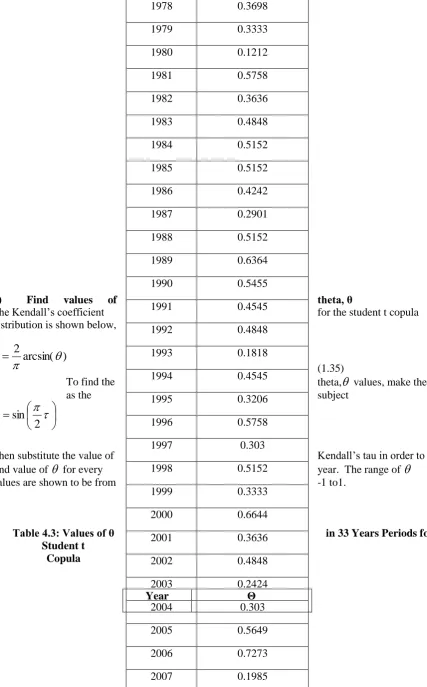
ii) Find values of theta, θ
The Kendall’s coefficient for the student t copula
distribution is shown below,
) arcsin(
2
(1.35)
theta, values, make the To find the
as the subject
Then substitute the value of Kendall’s tau in order to
find value of for every year. The range of
values are shown to be from -1 to1.
Table 4.3: Values of θ in 33 Years Periods for
Student t Copula
1978 0.3698
1979 0.3333
1980 0.1212
1981 0.5758
1982 0.3636
1983 0.4848
1984 0.5152
1985 0.5152
1986 0.4242
1987 0.2901
1988 0.5152
1989 0.6364
1990 0.5455
1991 0.4545
1992 0.4848
1993 0.1818
1994 0.4545
1995 0.3206
1996 0.5758
1997 0.303
1998 0.5152
1999 0.3333
2000 0.6644
2001 0.3636
2002 0.4848
2003 0.2424
2004 0.303
2005 0.5649
2006 0.7273
2007 0.1985
Year Θ
1975 -0.09505
1976 0.723787
1977 0.499955
1978 0.54876
1979 0.499955
1980 0.189233
1981 0.786094
1982 0.540593
1983 0.690024
1984 0.723787
1985 0.723787
1986 0.618107
1987 0.44008
1988 0.723787
1989 0.841284
1990 0.755796
1991 0.654807
1992 0.690024
1993 0.281705
1994 0.654807
1995 0.482579
1996 0.786094
1997 0.458184
1998 0.723787
1999 0.499955
2000 0.86424
2001 0.540593
2002 0.690024
2003 0.371627
2005 0.775397
2006 0.90965
iii) Find Degree of Freedom, v
In dependent t-test for paired samples, in which two samples are matched or paired, the degree of freedom used is n-1. Since there are 12 samples for every year, thus, the degree of freedom is 11.
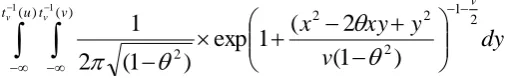
iv) Find Real Values of C(u,v)
By substituting the real values of u, v, θ and degree of freedom for every year into Eq.1.34, the values of copula will be obtained.
dy
v
y
xy
x
v v
t u tv v
2 1
2 2 2
) (
2 )
(
)
1
(
2
(
1
exp
)
1
(
2
1
11
The values of copula must be in range between 0 and 1.
Table 4.4: The Real Values of Student t Copula for 33 Years Period
i Year Ci(u,v)
1 1975 0.7004
2 1976 0.4643
3 1977 0.0182
4 1978 0.3969
5 1979 0.4772
6 1980 0.077
7 1981 0.2471
8 1982 0.616
9 1983 0.9955
10 1984 0.8352
11 1985 0.0211
12 1986 0.6862
13 1987 0.7622
14 1988 0.1247
15 1989 0.6683
16 1990 0.2646
17 1991 0.4275
Simulation experiment
The procedure is divided into two parts: Part 1 – finding the theoretical copula values. Part 2 – comparing the analysis of empirical copula and theoretical copula.
i) Generate 100 simulated data for the multivariate-t distributed.
100 random numbers are generated. The degree of freedom is 11 using the formula of n-1. The correlation coefficients is calculated using the Kendall’s tau of original data. The Kendall’s tau between distribution in Malacca and Tangkak is calculated using eq. (1.32) which gives the value 0.405. The PDF for multivariate-t distribution is given by
2 1
) ( )' ( 1 | | 2
2 )
)( , , (
d v
d td
v x P x
P v v
d v x
P v f
where v is degree of freedom, d is dimensional random vector and
is the gamma function. ii) Transform generated multivariate-t data to uniform data using marginals of univariate tdistribution
19 1993 0.823
20 1994 0.3194
21 1995 0.706
22 1996 0.0981
23 1997 0.8425
24 1998 0.3885
25 1999 0.3352
26 2000 0.5204
27 2001 0.6864
28 2002 0.1888
29 2003 0.5138
30 2004 0.0017
31 2005 0.4667
32 2006 0.0099
The PDF for univariate student’s t distribution is given by 2
/ ) 1 ( 2 1 ) 2 / ( 2
1
) (
v
v x v
v v x
f
where
defines a gamma function and vis degrees of freedom.The Kendall’s tau between distribution in Malacca and Tangkak is calculated using eq. (1.32) gives the value of 0.405. Then, substitute the value of Kendall’s tau into eq. (1.33) to get the value of θ such as below:
2 sin
0.405
2 sin
594121
.
0
iii) Eq (1.34) belowis used to calculate t copula . The range of these copula values must be in between 0 and 1.
dydx
v
y
xy
x
v v
t u
tv v 1 2
2 2 2
) (
2 )
(
)
1
(
2
(
1
exp
)
1
(
2
1
11
Comparing The Analysis Of Empirical Copula And Theoretical Copula.
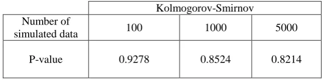
In this case, use Kolmogorov-Smirnov goodness of fit test to compare the distributions of the empirical and theoretical copula. The P-value is found to be greater than 0.05 significance level for this test, therefore the conclusion that the two distributions are not significantly different at 5% significance level can be made. For addition, 1000 and 5000 random numbers are generated to test the P-value. See table below:
Table 4.6: Goodness of fit test of theoretical and empirical copulas for the uniformised observed and generated data
Kolmogorov-Smirnov Number of
simulated data 100 1000 5000
P-value 0.9278 0.8524 0.8214
Two sets of data (two stations) were tested using Kolmogorov-Smirnov fit test to find the best fit marginal distributions. Lognormal provided the best fitted for station in Malacca and weibull was the best fitted for station in Tangkak. The parameters u,v, and degree of freedom were calculated in modelling the bivariate distribution. All calculated parameter values are within the acceptable range. Then, the bivariate joint distribution of rainfall data for student-t copula is computed. The simulation process of student-t copula has been carried out by using 100, 1000 and 5000 numbers of simulated data. All these simulations process give good results which their P-values are greater than 0.05 significance level.Therefore, every simulation distribution is not significantly different with the distribution of observed data.
1.6 CONCLUSION
Based on the Kolmogorov-Smirnov goodness-of-fit test, lognormal provided the best fitted distribution for station in Malacca and weibull was the best for station in Tangkak
The distributions of observed data and simulated data were not significantly different at 5% significance level Kolmogorov-Smirnov goodness of fit test
Results showed that all calculated parameter values were within the acceptable range and could be applied to compute the bivariate joint distribution of rainfall data for the student-t copula.
ACKNOWLEDGEMENT
The authors wish to thank Malaysia Meteorological Services for allowing us to do analysis on the climate data.
REFERENCES
Defu, L., Shuqin, W. and Liping, W. (2002). Poisson-Gumbel Mixed Compound Distribution and its application. Chinese Science Bulletin. 47(22): 1901-1906.
Kelly, K.S. and Krzysztofowicz, R. (1997). A bivariate meta-Gaussian density for use in hydrology. Stochastic Hydrology and Hydrailics. 11(1):17-31.
Nikoloulopoulos, A.K., H, Joe, H. and Haijun Li (2010). Vine copulas with asymmetric tail dependence and applications to financial return data. Computational Statistics & Data Analysis. 56(11), 3659-3673.
Quesada-Molina, J.J., Rodr´ıguez-Lallena, J.A., and Ubeda-Flores, M. (2003). What are copulas? Monograf´ıas del Semin. Matem. Garc´ıa de Galdeano. 27(3), 499-506.
Salarpour, M., Yusop, Z., Yusof, F., Shahid, S. and Jajarmizadeh, M. (2013). Flood frequency analysis based on t-copula for Johor River, Malaysia. Journal of Applied Sciences. 13(7), 1021-1028.
Schmidt, T. (2006). Copulas-From Theory to Applications in Finance. (1st ed.), London: Risk Books. Sklar, A. (1959). Functions de repartition an dimensionset leursmarges. (8th ed.), Paris: PublInst
Stat. Univ.
Yue, S., Ourda, T.B.M.J., Bobee, B., Legendre, P., and Bruneau, P. (1999). The Gumbel mixed model for flood frequency analysis. Journal of Hydrology. 226 (1-2): 88-100.
Yue, S. (2000). The Gumbel mixed model applied to storm analysis. Water Resources Management. 14(5): 377-389.