ABSTRACT
BUSH, BRETT ALAN. Analysis of Fuel Consumption for an Aircraft Deployment with Multiple Aerial Refuelings. (Under the direction of Thom J. Hodgson.)
The purpose of the research has been to derive an algorithm that finds optimal aerial refueling segments (non-instantaneous) for a single aircraft deployment while also accounting for atmospheric winds. There are two
decision variables: (1) Where to locate the refueling
segments? (2) How much fuel to offload at each refueling segment? Later in the dissertation, a third decision
variable is explored: How much fuel to load onto the aerial refueling aircraft?
In previous research, the problem of having a single aircraft deployment with one instantaneous aerial refueling has been explored and solved. This paper piggybacks on that research and extends it. The first step (Problem P1) is deriving an algorithm that finds the optimal aerial refueling points for a single aircraft deployment with
multiple instantaneous aerial refuelings. In the next step (Problem P2), one assumes aerial refueling is not
refueling segments are found (versus optimal refueling points). In the last problem (P3), one looks at a very similar algorithm that factors the winds aloft into the minimization algorithm. Finally, this paper looks at three distinct deployment scenarios with two aerial refuelings required. All of the scenarios were first planned by the U.S. Air Force and the results given to the author.
ANALYSIS OF FUEL CONSUMPTION FOR AN AIRCRAFT DEPLOYMENT WITH MULTIPLE AERIAL REFUELINGS
by
BRETT ALAN BUSH
A dissertation submitted to the Graduate Faculty of North Carolina State University
in partial fulfillment of the requirements for the Degree of
Doctor of Philosophy
OPERATIONS RESEARCH
Raleigh 2006
APPROVED BY:
Jeffrey R. Thompson Michael G. Kay
Russell E. King Yahya Fathi
BIOGRAPHY
After graduating from high school at Adirondack Central School in Boonville, NY in 1993, Brett Bush attended the United States Air Force Academy in Colorado Springs, CO. In 1997, he graduated with a Bachelor of Science in Mathematical Science and was commissioned as a second lieutenant in the U.S. Air Force. His first assignment was to the 49th Test and Evaluation Squadron at Barksdale AFB, LA to perform analysis on U.S. Air Force bomber weapon systems. In 2000, he was reassigned to Hanscom AFB, MA where he worked on modeling, simulation, analysis, and systems integration of Air Force C4ISR systems. While at Hanscom AFB, Brett attended
Northeastern University and obtained a Master of Science in Operations Research. In 2003, the Air Force reassigned him to Raleigh, NC to attend North Carolina State University and
ACKNOWLEDGEMENTS
I would like to thank Dr. Thom Hodgson for his guidance and wisdom which have been second to none. It has been a privilege to work under him. I also would like to thank my other committee members, Dr. Jeffrey Thompson, Dr. Michael Kay, Dr. Russell King, and Dr. Yahya Fathi for their time and help. Finally, I would like to thank my wife. Without her love and support, I could never have completed this research and doctoral program.
TABLE OF CONTENTS
LIST OF TABLES...v
LIST OF FIGURES...vi
CHAPTER I: INTRODUCTION...1
CHAPTER II: FUEL CONSUMPTION FUNCTION...9
CHAPTER III: PROBLEM (P1) – MODEL AND SOLUTION...25
CHAPTER IV: PROBLEM (P2) – MODEL AND SOLUTION...36
CHAPTER V: PROBLEM (P3) – MODEL AND SOLUTION...41
CHAPTER VI: ANALYSIS OF THE ALGORITHM...52
CHAPTER VII: FUTURE RESEARCH...60
REFERENCES...62
LIST OF TABLES
Table 2-1 C-5 Summary of Fit...13
Table 2-2 C-5 Analysis of Variance...13
Table 2-3 C-5 Parameter Estimates...13
Table 2-4 C-5 Effect Tests...13
Table 2-5 KC-10 Summary of Fit...16
Table 2-6 KC-10 Analysis of Variance...16
Table 2-7 KC-10 Parameter Estimates...16
Table 2-8 KC-10 Effect Tests...16
Table 5-1 Example Mercator Grid Lines...48
Table 5-2 Example Spherical Grid Lines...49
Table 6-1 Base Information...53
Table 6-2 CMARPS Data Results...53
Table 6-3 CMARPS Fuel Consumption...54
Table 6-4 Mission Parameters...54
Table 6-5 Algorithm Data Results...54
Table 6-6 Algorithm Fuel Consumption...55
Table 6-7 Effect of Reserve Fuel on Fuel Consumption...55
Table 6-8 Comparison...56
Table 6-9 KC-10 Fuel Utilization...58
Table 6-10 New Initial KC-10 Fuel Allocations...58
LIST OF FIGURES
Figure 1-1 Graphical Representation of P1...3
Figure 1-2 Graphical Representation of P2/P3...4
Figure 2-1 Sample Fuel Flow Chart...12
Figure 2-2 Residual by Predicted Plot...14
Figure 2-3 Normal Probability Plot of Residuals...14
Figure 2-4 C-5 Actual vs Predicted (Altitude)...15
Figure 2-5 C-5 Actual vs Predicted (Gross Weight)...15
Figure 5-1 Problem P3 Illustration...46
CHAPTER I
INTRODUCTION
Problem Description
In today’s world, the ability to deploy aircraft,
supplies, and manpower is an essential tenet to military
power. Often, the deployment distance will be outside the
range of the aircraft. This is usually overcome through the
use of aerial refueling. Sometimes, more than one refueling
will be required. This dissertation deals almost exclusively
with that possibility (although the algorithm also works for
one refueling).
The objective is to determine the optimal points on the
earth in which to refuel during a deployment from an origin
base to a destination with more than one refueling required.
This will also produce another decision variable: the amount
of fuel to offload at each refueling point. We will look at
three special cases of this problem.
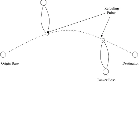
Problem (P1): There are N refuelings required for one
aircraft to go from origin base, A, to destination base, B and
N refuelings will occur with one tanker from each of N
refueling bases. A visual interpretation of this problem is
presented in figure 1-1.
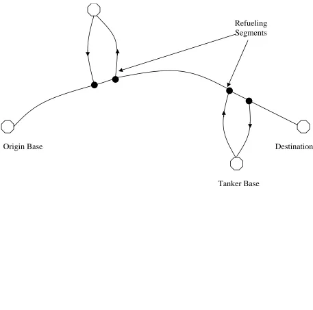
Problem (P2): There are N refuelings required for one
aircraft to go from base A to base B, and the refueling occurs
in such a way that it is not instantaneous, but requires time
to offload from the tanker to the deployment aircraft. The N
refuelings will occur with one tanker from each of N refueling
bases. A visual interpretation of this problem is presented
in figure 1-2.
Problem (P3): This is the same problem represented in Problem
(P2) except we will now account for winds aloft in determining
the optimal route.
These three problems successively build upon one another, as
problem (P1) must be solved in order to solve problem (P2).
Likewise, the algorithm for problem (P2) lays the foundation
for the solution of problem (P3).
Literature Survey
The problems described above all involve finding a
solution to a nonlinear minimization problem with constraints
due to the fact that the optimization takes place on a sphere
Tanker Base
Origin Base Destination
Tanker Base
Refueling Points
Tanker Base
Origin Base Destination
Tanker Base
Refueling Segments
previously stated problems are all an extension of a problem
solved by Yamani11. He solved the generic problem involving N
aircraft deploying with one refueling required. This paper
will use his solution to that problem and extend it to N
refuelings and show that this problem also converges to an
optimal solution. This problem, in its simplest form, can be
characterized as a location problem on a sphere.
Yamani’s work utilizes other significant results to
achieve a solution. A similar problem is the spherical Weber
problem with maximum distance constraints; however, that
particular objective function is linear. Aly1 showed that the
search for an optimal solution to the spherical Weber problem,
where demand points are not located entirely on a great
circle, is contained within a convex hull of the demand
points. Drezner5 proved if the demand points lie on a great
circle, the optimal solution also lies on this great circle.
Katz and Cooper7 showed the sufficient conditions under which
a demand point is a local minimum.
Some work has also been accomplished on the Weber problem
without constraints. Aly and Litwhiler8 solved this problem
using two different methods: the Map Projection Algorithm and
Cyclic Search Algorithm. Ayken2 derived the Cyclic Meridian
Parallel Search and Geodesic Descent Algorithm to solve the
converge to local optima as long as the search is limited to a
spherical radius of π/4. Additionally, it should be noted
that the optimal point may not be unique.
Some researchers have looked at how to solve the problem
with constraints. Love9 developed a process that handled
constraints through use of convexity and penalty functions.
Ayken2 found a solution to the Weber problem with distant
constraints given that the solution is within a certain
distance of previously known points.
Finally, Darnell and Loflin3,4 used linear programming to
solve a similar problem that utilized ground refueling, fixed
intermediate stops, and a return to the origin. Waite10 used
stochastic dynamic programming to solve a similar problem.
These problems had unrestricted but fixed refueling points
with different fuel costs.
Assumptions
Some assumptions need to be made in order to start the
solution process to these problems. These assumptions follow:
1. Aircraft will fly a great circle distance between any
solution points found. The algorithm will use a
version of the law of haversines to calculate this
distance. This calculation is a very good first order
calculation of the actual distance on the earth. This
Matlog toolbox. This takes the earth’s bulge into
account when performing calculations. The haversine
calculation follows12:
=
=
= + × ×
= ×
= ×
3 958 75
2 1
2 1
sin 2 cos 1 cos 2 sin 2
2 tan 2 1
R earth's radius ( , . mi)
Δlat = lat - lat
Δlong long - long
a ²(Δlat/ ) (lat ) (lat ) ²(Δlong/ )
c a ( a, ( - a))
d R c
2. Weather at altitude is assumed to be negligible except
in Problem (P3).
3. All deploying aircraft are of the same model.
Similarly, the refueling aircraft are all assumed to
be of the same model. In the particular algorithm
being developed, the deploying aircraft is a C-5 and
the refueling aircraft is a KC-10. If a requirement
arises to analyze different types of aircraft beyond
these, all that would be required is to change the
fuel consumption functions introduced in chapter II.
4. For the non-instantaneous problems (P2) and (P3),
aircraft fuel consumption will be a constant during
refueling segments due to the fact gross weight will
be changing negatively due to fuel consumption AND
5. Takeoff and landing fuel consumption as well as
position where these events occur will be input by the
user and treated as constants.
6. Cargo weight must meet aircraft gross weight
requirements also taking into account the fuel weight.
7. All aircraft will operate at a 99% maximum specific
fuel rate, as this will ensure maximum speed while
being only 1% less than the best fuel efficiency.
8. Aircraft are assumed to require a safety stock of
fuel. This requirement affects range calculations,
making the aircraft’s effective range decrease. (due
to the fact the safety stock fuel cannot be used for
CHAPTER II
FUEL CONSUMPTION FUNCTION
Fuel Consumption Rate Function
In this chapter, we derive formulas for fuel consumption
and aircraft range based on cargo weight (w0), initial fuel (g0
for deploying aircraft/h0 for refueling aircraft), and flight
altitude (alt). Yamani11 derived these equations in the same
manner with one notable difference. His equations depended
solely on the gross weight of the aircraft. The following
equations also incorporate flight altitude, as that was also
deemed a significant factor in the model after performing the
regression analysis.
The data is based on information in technical order
1C-5A-1-115 for the deploying aircraft and the KC-10A performance
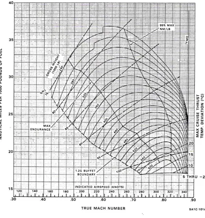
manual14 for the refueling aircraft. Figure 2-1 shows an
example specific range chart for the KC-10A at an altitude of
29,000 feet. These range charts exist for various altitudes.
It is necessary to model the fuel consumption rate information
In order to do that, we will assume the aircraft operates at
the 99% specific range since this maximizes velocity and is
near optimal in fuel consumption.
Let
MPF(GW, Alt) = the distance traveled in miles per 1,000
lbs of fuel burned given the aircraft
gross weight, GW, and the flight altitude,
Alt
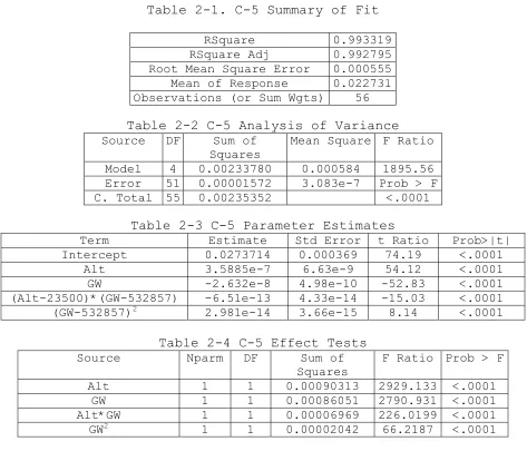
Tables 2-1, 2-2, 2-3, 2-4, and 2-5 show fit, ANOVA, estimates,
and effects tests based on the data from the C-5. A second
degree polynomial model is used. We can see this gives an
adjusted R2 of over .99 which gives a sufficiently accurate
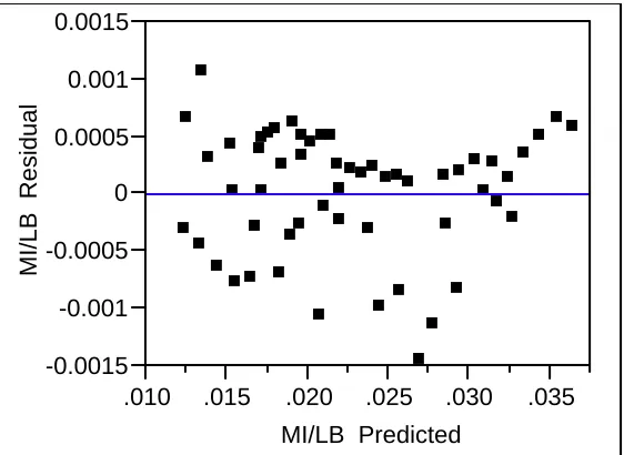
representation of the data. Figure 2-2 shows a plot of the
residuals of the data. We can see that the mean of the
residuals is around zero and appear to be random which
indicates a good model for our data. The KC-10 fuel
consumption rate model also has an adjusted R2 over .99 and is
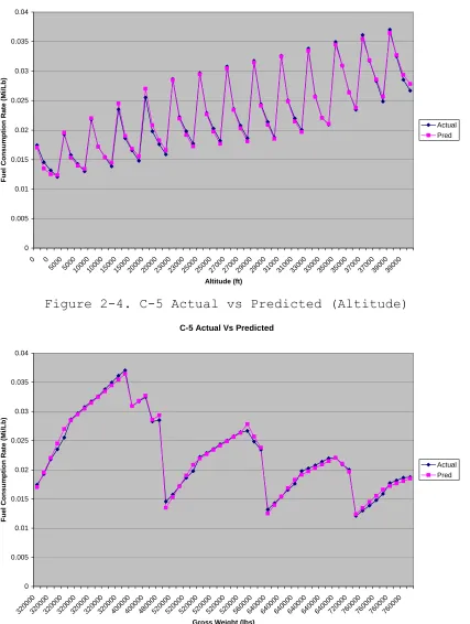
derived similarly. Figures 2-4 and 2-5 are plots of the
actual versus predicted MPF(GW,Alt) against various altitudes
and gross weights for the C-5 data. Notice in figure 2-4, the
x-axis has four data points for every altitude. The four data
points associated with each altitude are taken at
progressively heavier gross weights. Thus, that is the reason
altitude. However, you will notice the general trend is an
increase in altitude corresponds to a decrease in fuel
consumption rate. In figure 2-5, you will notice the x-axis
has multiple repeating entries for different gross weights.
This is due to the fact that the data points taken at these
particular gross weights are taken at different altitudes.
The general trend is for the fuel consumption rate to decrease
as gross weight increases. The computed models of MPF(GW,
Alt) for the C-5 and KC-10 follow: (note that Alt2 did not
turn out to be a significant factor for the C-5)
MPFC-5(GW, Alt)
× ×
× × × 2
0.27678e-1+0.70599e-6 Alt-0.42783e-7 GW
-0.65146e-12 Alt GW+0.29811e-13 GW
MPFKC-10(GW, Alt)
+ × + ×
× × ×
+ ×
2 2
-0.2976658738 - 1 0.4268994944 - 5 0.1481265454 - 7 -0.4203287222 - 11 - 0.3626383552 - 10
0.6426861944 - 13
e e Alt e GW
e Alt GW e Alt
Table 2-1. C-5 Summary of Fit
RSquare 0.993319
RSquare Adj 0.992795
Root Mean Square Error 0.000555
Mean of Response 0.022731
Observations (or Sum Wgts) 56
Table 2-2 C-5 Analysis of Variance
Source DF Sum of
Squares Mean Square F Ratio
Model 4 0.00233780 0.000584 1895.56
Error 51 0.00001572 3.083e-7 Prob > F
C. Total 55 0.00235352 <.0001
Table 2-3 C-5 Parameter Estimates
Term Estimate Std Error t Ratio Prob>|t|
Intercept 0.0273714 0.000369 74.19 <.0001
Alt 3.5885e-7 6.63e-9 54.12 <.0001
GW -2.632e-8 4.98e-10 -52.83 <.0001
(Alt-23500)*(GW-532857) -6.51e-13 4.33e-14 -15.03 <.0001
(GW-532857)2 2.981e-14 3.66e-15 8.14 <.0001
Table 2-4 C-5 Effect Tests
Source Nparm DF Sum of
Squares F Ratio Prob > F
Alt 1 1 0.00090313 2929.133 <.0001
GW 1 1 0.00086051 2790.931 <.0001
Alt*GW 1 1 0.00006969 226.0199 <.0001
-0.0015 -0.001 -0.0005 0 0.0005 0.001 0.0015
MI/LB Residual
.010 .015 .020 .025 .030 .035
MI/LB Predicted
Figure 2-2 (Residual by Predicted Plot)
.01 .05 .10 .25 .50 .75 .90 .95 .99
-3 -2 -1 0 1 2 3
Normal Quantile Plot
-0.0015 -0.0005 0 .0005 .001 .0015
C-5 Actual Vs Predicted MPF 0 0.005 0.01 0.015 0.02 0.025 0.03 0.035 0.04 0 0 500 0 500 0 1000 0 1000 0 1500 0 1500 0 2000 0 2000 0 2300 0 2300 0 250 00 2500 0 2700 0 270002900
0 2900 0 3100 0 3100 0 3300 0 3300 0 3500 0 3500 0 3700 0 3700 0 3900 0 3900 0 Altitude (ft) Fue l C o n s u m pt ion R a te (M i/ Lb) Actual Pred
Figure 2-4. C-5 Actual vs Predicted (Altitude)
C-5 Actual Vs Predicted
0 0.005 0.01 0.015 0.02 0.025 0.03 0.035 0.04 3200 00 3200 00 3200 00 3200 00 3200 00 3200 00 3200 00 400 000 4000 00 4800 00 520 000 5200 00 5200 00 52000 0 5200 00 5200 00 5600 00 6400 00 6400 00 6400 00 640 000 6400 00 6400 00 720 000 7600 00 7600 00 76000 0 7600 00
Gross Weight (lbs)
Fue l C ons um pti on R a te (M i/ Lb) Actual Pred
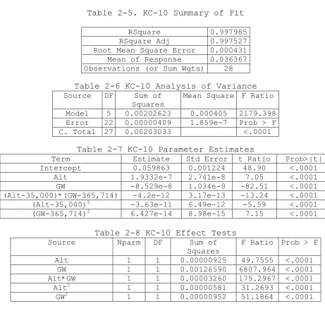
Tables 2-5, 2-6, 2-7, and 2-8 show the regression analysis for
the KC-10 fuel flow function.
Table 2-5. KC-10 Summary of Fit
RSquare 0.997985
RSquare Adj 0.997527
Root Mean Square Error 0.000431
Mean of Response 0.036367
Observations (or Sum Wgts) 28
Table 2-6 KC-10 Analysis of Variance
Source DF Sum of
Squares Mean Square F Ratio
Model 5 0.00202623 0.000405 2179.398
Error 22 0.00000409 1.859e-7 Prob > F
C. Total 27 0.00203033 <.0001
Table 2-7 KC-10 Parameter Estimates
Term Estimate Std Error t Ratio Prob>|t|
Intercept 0.059863 0.001224 48.90 <.0001
Alt 1.9332e-7 2.741e-8 7.05 <.0001
GW -8.529e-8 1.034e-9 -82.51 <.0001
(Alt-35,000)*(GW-365,714) -4.2e-12 3.17e-13 -13.24 <.0001
(Alt-35,000)2 -3.63e-11 6.49e-12 -5.59 <.0001
(GW-365,714)2 6.427e-14 8.98e-15 7.15 <.0001
Table 2-8 KC-10 Effect Tests
Source Nparm DF Sum of
Squares F Ratio Prob > F
Alt 1 1 0.00000925 49.7555 <.0001
GW 1 1 0.00126590 6807.964 <.0001
Alt*GW 1 1 0.00003260 175.2967 <.0001
Alt2 1 1 0.00000581 31.2693 <.0001
Aircraft Range Function
It is important to know the distance, d, an aircraft can
fly given its initial fuel (g0), flight altitude (alt), and
cargo weight (w0). First, let us consider the initial gross
weight (GW) of the aircraft.
GW = EW + g0 + w0 (note that this formulation only holds
true if the aircraft has not used any fuel yet)
where EW is the empty weight of the aircraft. During flight,
GW = EW + f + w0
where f is the amount of fuel left. One can easily see that
EW and w0 do not change. Therefore,
∂GW = ∂f
Let
Rj(g0, w0, alt) = the range of aircraft j given an initial
fuel, cargo weight, and flight altitude
Now, we can surmise that an optimal solution will occur only
if the deploying aircraft finishes with little or no fuel.
Therefore, the ending gross weight is,
Final GW = EW + w0 (as f = 0)
We can now integrate the MPF(GW, Alt) function we found
earlier for each aircraft and find its range function:
) , ,
(g0 w0 alt
R
+ +
+
=
∫
0 00
( )
EW w g
EW w
∫
+ + = 0 0 0 ) ( g df f w EW MPFWe get the following:
RC-5(g0,w0,alt):
× × × × + × × + × × + × + × × × × × × 3 2 2 2 2 0 0 0 0
0 0 0
0 0
0 0
0.9937160432 - 14 - 0.2139143481 - 7
-0.3257322132 - 12 0.2981148130 - 13 0.2981148130 - 13 0.2767819883 - 1 0.7059890563 - 6 - 0.4278286962 - 7 -0.4278286962 - 7
-e g e g
e g Alt e g EW
e g w e g
e Alt g e EW g
e w g × × ×
× × × + × ×
+ × × × + × × 2
0
2
0 0 0
0 0 0 0
0.6514644265 - 12
-0.6514644265 - 12 0.2981148130 - 13 0.5962296260 - 13 0.2981148130 - 13
e g Alt EW
e g Alt w e g EW
e g EW w e g w
RKC-10(h0,y0,alt):
× × × + × + × × + × × × + × × + × × + × × + 3 2 0 0 2 2 0 0 2
0 0 0
0 0
0 0
0.2142287315 - 13 - 0.2101643611 - 11 0.7406327270 - 8 0.6426861945 - 13 0.6426861945 - 13 - 0.2976658738 - 1 0.4268994944 - 5 0.1481265453 - 7 0.1481265453 - 7
e h e h Alt
e h e h EW
e h y e h
e Alt h e EW h
e y h × ×
+ × × × + × × × × × × × × × × 2 0 2
0 0 0 0
0 0 0
2 0
0.6426861944 - 13
0.1285372389 - 12 0.6426861944 - 13 -0.4203287222 - 11 - 0.4203287222 - 11 -0.3626383552 - 10
e h EW
e h EW y e h y
e h Alt EW e h Alt y
e h Alt
Fuel Consumption Function
It is also helpful to know Fj(g0, w0, alt, d), the amount
of fuel consumed when an aircraft flies a given distance, d,
with an initial fuel, g0/h0, flight altitude, alt, and cargo
weight w0/y0. In order to find this value, we must also know
how much fuel is left in the aircraft after completion of the
leg. We will denote this value as g1/h1. Now,
1 0
0
0, w, alt, d) g - g
(g
Since we know g0, we must only find g1 in order to find Fj(g0,
w0, alt, d). We do this through the following equation,
∫
+ +=
0
1
)
( 0
g
g
Doing this, we get the following:
FC-5(g0, w0, alt, d):
+ × × + × × × × + × + × + × × + × × + × 2 0 0 0 0 0 0
(-141131967 0.3950720052 19 -141131967 - 0.2053949494 13 -0.2053949494 13 0.1449491222 15
(0.8215797968 33 0.5797558638 21 0.8437417038 25 0.8437417038 25
g Alt w e
Alt EW e EW
e w e Alt
sqrt e d e Alt g
e EW g e w ×
+ × + × × × + × × × + × + × × + × × × × × 2 0 0 2 2 0 2 0 2 0
0.1145306807 34 0.1159511729 22
0.3983646422 17 0.2101024802 29 0.5645278680 29 0.1991823211 17
-0.4091390946 23 - 0.1622915890 32 -0.1622915890
g
e Alt e Alt w EW
e Alt EW g e Alt
e Alt d e Alt g
e Alt g e EW
× + × + × + × × × + × × × + × × × × × × × 2 0 0 0 0 0 0 2 0 0
32 0.1560818893 38 -0.1622915889 32 0.4218708516 25
0.1159511728 22 0.1159511728 22 0.3983646422 17
-0.1710582136 28 - 0.1710582136 28 -0.1710582136
e w e
e g e g
e Alt EW g
e Alt w g
e Alt w EW
e Alt g e Alt EW
e × × + × × ×
+ × × + × × × × + × × + × × × × + × 2 2 2
0 0 0
2
0 0
2 2 2
0
2 2
28 0.3983646422 17
0.1991823211 17 0.5797558643 21 -0.4091390946 23 0.1991823211 17
0.5797558643 21 - 0.4091390946 23 0.4218708522 25
Alt w e Alt w g
e Alt w e Alt w
e Alt w e Alt EW
e Alt EW e Alt EW
e E + × ×
+ × 2 ÷ + ×
2
0 0
0.8437417044 25
0.4218708522 25 )) (0.2053949492 13 141131967 )
W e EW w
FKC-10(h0, y0, alt, d): + × × × + × × + × × × × × × × × × 0 0 0 0 0 0
(0.8539003945 16 - 0.1499862837 14 -0.6936177892 12 - 0.6936177892 12
38507457.01 38507457.01 -0.7812500000 - 2 (-0.1750430987 25 -0.1750430987 25 - 0.41967074
h e e Alt
e EW e y
Alt EW Alt y
e sqrt e EW Alt h
e y Alt h ×
+ × × + × ×
+ × × + × ×
+ × × ×
× ×
× +
0 0 0
0 0
0 0
28 34 0.1576486953 29 0.1576486953 29 0.3516704614 30 0.3516704613 30 0.3516704613 30 - 0.1775661541 36 -0.1940784755 33 - 0.1940784755 33
-0.1940784756 33 0.
e Alt
e EW h e y h
e Alt h e Alt EW
e Alt y e d
e EW e y
e h ×
× × + + × × × × × × + × × × + × × × + × 2 2 0 0 2 0 0 2 2
0 0 0
2
7882434769 28
-0.8752154935 24 0.1194632616 37 0.4858918487 20 - 0.1750430987 25 0.4858918486 20 0.4858918486 20 0.3685725846 31 - 0.1892545453 2
e h
e Alt h e
e Alt EW y e EW Alt y
e y Alt h e EW Alt h
e Alt e × ×
× × + × + × × × × + × × × + × × + × × + 2 2 2 2 2 2 0 2 0 0 0
2 2 2
0 6
-0.1892545453 26 0.7882434765 28 0.1576486953 29 - 0.8752154935 24 0.7882434765 28 - 0.8752154935 24
0.2429459243 20 0.2429459243 20 0.2429
Alt EW
e Alt y e EW
e EW y e Alt EW
e y e Alt y
e Alt EW e Alt y
× × + × × × × ÷ + × 2 2 0 2 0
459242 20 0.9857908992 31
-0.1892545452 26 )) (-0.6936177894 12 38507457 )
e Alt h e Alt d
e Alt h e Alt
The above equations are based on the quadratic model with no
two way interactions considered of the fuel consumption rate
equation. The adjusted R2 was about .989 and .985 for the
KC-10 and C-5 models, respectively.
From the research performed by Yamani, we know the fuel
consumption function is a concave and increasing function of
the distance11. Additionally, the fuel consumption function is
Fuel Requirement Function
The last function of interest is the fuel requirement
function, FRj(w0, alt, d). This function represents the exact
amount of fuel required to fly a distance, d, at flight
altitude, alt, and cargo weight, w0. We know the initial
amount of fuel, g0/h0 must be greater than or equal to the fuel
required (otherwise the aircraft would run out of fuel). So,
set
Rj(g0,w0,alt) = d
FRC-5(w0, alt, d): × + + × × × × × × + × × × + × + 2 0 0 0
(-0.2053949494 13 0 0.3950720052 19
0.1449491222 15 - 0.2053949494 13
-141131967.0 - 141131967.0
(0.1145306807 34 - 0.1622915890 32
-0.1622915890 32 0.4218708522 25
0.8
e w e
e Alt e EW
Alt EW Alt w
sqrt e Alt e EW
e w e w
× × + × × + × × × × × + × + × × + × × + × 2 0 0 2 2 2 2 0
2 2 2
437417044 25 0.5797558643 21
0.2101024802 29 - 0.4091390946 23
-0.4091390946 23 0.4218708522 25
0.5797558643 21 0.1991823211 17
0.1991823211 17
e w EW e Alt w
e Alt e Alt EW
e Alt w e EW
e Alt EW e Alt EW
e Alt × + × × ×
+ × × × + × × × × × × × ÷ + × 2 2 2 0 0 0 0 0.3983646422 17
0.1159511729 22 0.1560818893 38
-0.1710582136 28 - 0.1710582136 28
-0.8215797968 33
-0.5645278680 29 )) (0.2053949492 13 141131967 )
w e Alt EW w
e w Alt EW e
e Alt EW e Alt w
e d
FRKC-10(y0, alt, d):
× + ×
× + × ×
+ × × × × ×
× × 2 + ×
0
0 0
2 0
(-0.8878307702 14 0.1092992505 19 - 0.1919824431 16
-0.8878307702 14 4928954497
4928954497 - (0.1576486953 29
-0.8752154934 24 0.3685725846 31
-0.1892545453 26
e y e e Alt
e EW Alt EW
Alt y sqrt e y EW
e Alt y e Alt
e × × × ×
+ × × × + × × + × + + × × × × × × 2 2 2 0 2 2
2 2 2
0 2
0 0
- 0.1892545453 26
0.7882434764 28 - 0.8752154934 24
0.2429459243 20 0.2429459243 20 *
0.1194632616 37 0.4858918487 20
-0.1750430987 25 - 0.41
Alt EW e Alt y
e EW e Alt EW
e Alt EW e Alt y
e e Alt EW y
e y Alt EW ×
+ × × + × × × × + × + × × × ÷ + × 2 0 0 0 96707428 34
0.3516704613 30 0.3516704613 30
-0.1940784755 33 - 0.1940784755 33 0.7882434764 28
0.1775661541 36 - 0.9857908994 31 ))
(-0.8878307703 14 4928954497 )
e Alt
e Alt y e Alt EW
e EW e y e y
e d e d Alt
CHAPTER III
PROBLEM (P1)—MODEL AND SOLUTION
1 Aircraft
N Aerial Refuelings
(N+1 legs)
Instantaneous Refueling
Problem Description
This problem is an extension of a problem solved by
Yamani11. He considered and solved the problem for one aerial
refueling with the assumption that refueling is instantaneous.
Consider the case where there is one aircraft that is to be
deployed from base A to base B. However, the distance, d,
from base A to base B is greater than the range, Rdeploy(g0, w0,
alt), of the deploying aircraft. Therefore, 1 or more aerial
refuelings must be accomplished. The tanker aircraft would
come from predetermined air bases and refuel the deploying
aircraft in midair enroute to base B. At the end of each
refueling, the tanker aircraft would return to its origin
refueling points that minimize total fuel consumption of both
the deploying aircraft and the N tanker aircraft used.
Additionally, we shall determine how much fuel is added to the
deploying aircraft at each refueling point. Let
Di = the distance of leg i of the deployment
(for example, the distance from the origin
base to the first refueling point would be
D1 and the distance from refueling point 1
to refueling point 2 would be D2, etc.)
Ti = the distance from aerial refueling base i
to aerial refueling point i
Rj(g0, w0, alt) = the range of aircraft j given its initial
fuel, cargo weight, and planned flight
altitude (j = tanker or deploying
aircraft)
Fmax(w0, j) = the maximum fuel aircraft j can carry
given its cargo weight (j = tanker or
deploying aircraft)
Wmax(j) = the maximum gross weight for aircraft j (j
= tanker or deploying aircraft)
Fj(g0, w0, alt, d) = amount of fuel used to fly a distance d
given an initial fuel amount, cargo
weight, w0, and altitude by aircraft j (j
fi = amount of fuel consumed by the deploying
aircraft on leg i
xi = Fdeploy( 0 1 1 0
1 i
i j j
j
g (x − f − ),w ,D ,alt)
=
+
∑
−xi = amount of fuel transferred from the tanker
to the deploying aircraft at refueling
point i
ri = amount of fuel used by tanker aircraft i
to fly from its home base to the refueling
point
ri = FRtanker(h0,y0,Ti,alt)
si = amount of fuel used by tanker aircraft i
to fly from its refueling point back to
its home base
si = Ftanker(h0-xi-ri,y0,Ti,alt)
w0 = cargo weight of deploying aircraft
y0i = cargo weight of tanker aircraft i
g0 = initial fuel of deploying aircraft
h0i = initial fuel of tanker aircraft i
Several constraints must be satisfied in determining the
N optimal refueling points. First, the distance of each leg
cannot exceed the maximum range of the deploying aircraft.
0 1 1 0
1
( ( ), , )
i
i deploy j j j
D R g x− f − w alt
=
Second, the tanker aircraft must be able to reach the
refueling point and then have enough fuel to return back to
its original base. This algorithm will assume that getting to
the aerial refueling point is not a problem for the tanker,
however, the algorithm checks to make sure that there the
aerial refueling aircraft has enough range to make the trip
back to its home base from the aerial refueling point.
≤ tan ker( 0i − − Ftanker(h , y , T ),0i 0i i 0i, )
i i
T R h x y alt
Similarly, the amount of fuel consumed by both the tanker and
deploying aircraft for each leg must be less than either its
maximum fuel given its cargo weight, or for leg 1, less than
its initial fuel, g0 or h0:
0 0 1 0
0 1 1 0 0 1 1
1 1
tan ker 0
tan ker 0
( ( ), , , ) ( ) ( ) i i i i deploy i i
deploy j j i j j
j j
0 0 i
0 i i 0 i i i
F (g , w , alt, D , alt) g
F g x f w D alt g x f
F h , y ,T ,alt h
F h x r , y ,T ,alt h x r
− − − − = = ≤ + − ≤ + − ≤ − − ≤ − −
∑
∑
Additionally, the aircraft must meet its weight requirements
at each leg, i. Thus:
max 0 0 1 1
1
max 0i 0i
i
j j j
W (deploy) g w (x f )
W (tanker) h y
− −
=
≥ + + −
≥ +
Finally, it should be noted that the tanker aircraft must also
be able to offload the necessary fuel to the deploying
aircraft, while also being able to reach its final
destination.
Formulation of (P1)
The problem can be stated mathematically as follows: find
the N coordinates (latitude, longitude) and amount of fuel
transferred from the tanker to the deploying aircraft at each
refueling point that will
(P1) Minimize i i
N
i
i r s
f + +
∑
=1
s.t.
0 1 1 0 0 1 1
1 1
0 1 1 0
1
tan ker 0i 0 0i
i i
deploy j j i j j
j j
i
i deploy j j j
i
F (g (x f ),w ,D ,alt) g x f
D R (g (x f ),w ,alt)
F (h , y ,T ,alt) h
− − − − = = − − = + − ≤ + − ≤ + − ≤
∑
∑
∑
tan ker 0 0 0
tan ker 0 0
tan ker 0 tan ker 0 0 0
i i
i i
i i i i
i i i i i
i
i i i
F (h x r , y ,T ,alt) h x r
T R (h , y ,alt)
T R (h x F (h , y , T ), y ,alt)
− − ≤ − −
≤
≤ − −
max 0 0 1 1
1
max 0i 0i i
j j j
W (deploy) g w (x f )
W (tanker) h y
− −
=
≥ + + −
≥ +
∑
Note: the tankers are all assumed to be the same model, and
Solution Procedure for Problem (P1)
1. Pick N initial feasible points. (discussion of how to
pick these points is at the end of the chapter)
2. Calculate the fuel cost involved with using these N
initial feasible points.
3. Set an N length vector, λ (step length), a minimum λ, a
tolerance (TOL), and let i=1.
4. Fix all N points except for point i. Create four ‘new’
points by moving point i north, south, west, and east by λi.
a. Calculate the fuel cost of each of the four
‘new’ points and check feasibility.
1. If the ‘new’ point is not feasible, the
fuel cost associated with that point is
infinity.
b. Compare the smallest fuel cost of the four
‘new’ points to the ‘old’ fuel cost. If ‘new’
fuel cost < fuel cost, set point i to the point
corresponding to the ‘new’ fuel cost and fuel
cost is now equal to ‘new’ fuel cost. Set
difference = fuel cost – ‘new’ fuel cost.
1. Else, set λi= λi/2.
5. Check the vector λ against the minimum λ requirement
movement. If difference < TOL & max (λ) < (user
defined min λ), the algorithm is complete. If not,
continue.
6. Increment i unless i=N, then set i=1 again.
7. Go to step 4.
Yamani11, using the fact that the distance from a given point r
is an s-convex function within a circle of radius Π/2 and
center r (Drezner and Weslowsky6) and the search for an
optimal solution to the spherical Weber problem can be
restricted to the spherical convex hull of the demand points
(Aly1), showed that we can limit our search for refueling
points to the convex hull of the endpoints of each leg i,
along with the associated aerial refueling base point.
Yamani11 also showed that the objective function is s-convex.
The multiple aerial refueling problem is clearly just an
extension of the single refueling station problem. We can
apply the same procedure if we temporarily fix the points
before and after the refueling point of interest. Since the
objective function is s-convex, we know that if we move in a
direction that improves the objective function, we are moving
toward the optimal position. When it is no longer possible to
improve the objective function in any direction and/or step
Obtaining an Initial Feasible Solution
1. Let j=1 and start with the origin base, (xj-1, yj-1)
and first aerial refueling base, (ARxj,ARyj).
2. Let the jth refueling point be (zj, wj) = ((xj-1+ARxj)/2,
(yj-1+ARyj)/2) for all j initially. (Note that since this
is on a sphere, these interpolated points are not
midpoints. This does not matter for our purposes here.)
3. Check feasibility of the new found point.
a. If point j is too far from the aerial refueling base
(range of tanker, Rtanker(h0, y0, alt), is less than
the distance from the aerial refueling base to the
refueling point), move point j incrementally closer
to the aerial refueling base; ((9*zj + ARxj)/10,
(9*wj + ARyj)/10).
b. If point j is out of range of the deploying aircraft
(Rdeploy(g0, w0, alt)), move point j incrementally
closer to the previous refueling point or origin;
((xj-1+9*zj)/10, (yj-1 + 9*wj)/10).
c. If point j is out of range of the next refueling
point (or destination if j=N), move point j closer
to the next refueling point;
((xj+1+9*zj)/10, (yj+1 + 9*wj)/10).
4. If all points are feasible, you are complete. If not,
Convergence Proof for N>1 Aerial Refuelings
We need to show that at each and every successive
iteration, the total fuel consumption for both deployment and
refueling aircraft is less than or equal to the previously
calculated total fuel consumption. Yamani showed this is true
for N=1. Assume that we know the optimal solution of
refueling points, call this set S and it takes k iterations to
achieve. Now, also assume that at some iteration, i<k, the
calculated total fuel consumption increases (diverges).
Remember, the algorithm moves one refueling point at a time,
and fixes all other points. Let S’ be the solution set
associated with the i-1 iteration. According to the above
algorithm, if that were the case, we would not change S’ due
to the fuel cost increasing, and we would divide λj for point
j by 2 and perform the next iteration. Assume the total fuel
consumption keeps diverging for point j. Eventually λj would
be sufficiently close to zero and the ‘new’ points created by
moving a distance λj would be the same as the point in the
current solution set S’. Then S’(j)=S(j) and this point is in
the optimal solution set for point j. This same concept can
be shown to be true for all points of j from 1 to N.
Therefore, the objective function never increases from one
iteration to the next, and if it reaches a point where it
that could happen is the objective function maintains the same
value. Therefore, since Yamani11 showed the fuel consumption
functions are s-convex, we know via Drezner and Wesolowsky6
CHAPTER IV
PROBLEM (P2)—MODEL AND SOLUTION
1 Aircraft
N Aerial Refuelings
(N+1 legs)
Non-Instantaneous Refueling
Problem Description
This problem is the exact same one described in the last
chapter except for the fact that refueling is assumed to
consist of a start point and end point, instead of being an
instantaneous procedure. Therefore, this will mean that a
deployment will consist of 2N+1 legs. This chapter will
introduce a heuristic that will obtain a ‘near’ optimal
solution to the problem.
The mathematical formulation and solution procedure (at
least the start of it) of this problem is the same as Problem
Solution Procedure for Problem (P2)
1. Solve Problem (P2) using Problem (P1) method. This gives
you N instantaneous optimal refueling points. We will
call these (xi, yi) i=1..N. Let i=0.
2. Calculate the fuel remaining in the object aircraft at
point i using Fj(g0, w0, alt, d).
3. Calculate FRdeploy(w0, alt, Di+1). Once we have (2) and (3),
we know how much fuel we must offload from the tanker,
xi+1, in order to make the next refueling point by
calculating how much fuel we have left at point i,
Fdeploy(g0, w0, alt, Di), and also using FRdeploy(w0, alt,
Di+1), the fuel required to go from point i to point i+1.
The user will provide the program with an offload rate, α,
and a speed, β, can be calculated using regression based
on aircraft altitude and weight.
4. For the purposes of the refueling legs, fuel consumption,
γ, will be assumed to be constant on just those legs.
This is due to the fact that the fuel consumption
functions will not accurately predict fuel usage when the
weight of the aircraft is increasing in the middle of
flight (due to aerial refueling).
5. Once we have obtained (4) and also have a constant fuel
distance leg length. For each point i, we have a
refueling distance,
+
= ( 0 1 ÷
i i
q FR w , D , alt) α
Note: it is imperative when making these calculations that
you make sure your units match.
6. Next, we calculate 10 different refueling segments for
segment i and pick the best one in terms of fuel
consumption. (Note: the number of refueling segments may
change as I continue performing sensitivity analyses to
determine the number that maximizes performance and
efficiency of the algorithm.)
a.Bearing Calculation from point i+1 to point i:
∇ = + −
∇ = + −
= ∇ × +
× +
− × + × ∇
1 1)
tan 2 sin cos 1
cos sin 1
sin cos 1 cos
lon lon(i ) lon(i)
lat lat(i lat(i)
Br a ( ( lon) (lat(i ),
(lat(i) (lat(i )
(lat(i) (lat(i ) ( lon))
b.Calculation of a point given a bearing, Br, and
distance, d, from another point (use the
instantaneous refueling point):
= +
= +
1 sin sin cos os sin cos
1 tan 2 sin sin cos
cos sin sin 1
lat a ( (lat)* (d) c (lat)* (d)* (Br)); lon lon a (( (Br)* (d)* (lat)),
(d) - ( (lat)* (lat )));
This point is the beginning of the refueling segment.
Calculate this point for ki = (qi/10)*p where p = 1 to
7. Since we have found the beginning refueling point,
we must now find the end refueling point for each
refueling segment. Let A be the instantaneous refueling
point (xij, yij). Let B be the next instantaneous
refueling point (xi+1, yi+1). Let D be the beginning
refueling point, (a,b). Now, given a great circle route
AB and a point D, we can find the points on AB that lie a
distance qi from D. This will give us the ending
refueling point13.
a.M=bearing(AD)-bearing(AB)
L=dist(AD)
r= cos2(L)+ sin2(L)*cos2(M)
p = atan2(sin(L)*cos(M),cos(L))
dp = p +- acos(cos(qi)/r)
Repeat this for all D = ki and call this
solution point kki.
8. Now, check all 10 possible solutions for beginning and
ending refueling point i, and pick the segment that
minimizes fuel consumption and also meets range function
feasibility for both tanker and deployment aircraft.
Increment i and return to step 2. If i=N, go to step 10.
9. Set i=1. In the same way as Problem (P1), move the
beginning and ending refueling points for each i a fixed
10. If we can move the beginning and ending refuel points and
achieve a smaller fuel cost, the associated points are the
new beginning and ending refuel points for step i.
Otherwise, λi= λi/2.
11. Increment i or if i=N, set i=1 and goto step 10. Stop the
procedure when all λi are sufficiently small AND the
difference between fuel costs are negligible.
12. Repeat steps 6-8 again, checking if the angle of the
CHAPTER V
PROBLEM (P3)-MODEL AND SOLUTION
1 Aircraft
N Aerial Refuelings
Non-Instantaneous Refueling
Winds Aloft Factored into Fuel Cost Calculations
Problem Description
Suppose we have an aircraft that needs to be deployed
from base A to base B and the distance between the two bases
is greater than the range of the aircraft. Thus, 1 or more
aerial refuelings are required. There are predetermined
refueling bases from which refueling aircraft takeoff and land
to support these deploying aircraft en route to the
destination. In the real world, we must also account for
winds when flying our aircraft. A significant headwind causes
an aircraft to use more fuel than no wind or even, a tailwind.
The problem then is: where do the optimal refueling points
Solution Procedure
The procedure mimics the problem (P2) solution with one
notable exception: the actual calculation of the fuel cost.
Everything else remains the same.
Calculation of Fuel Cost
In problem (P2), we calculated fuel cost from the
equations derived in Chapter 2. We will still use these
equations to correct for wind, but we must modify the distance
traveled in order to compute the fuel cost.
1. Obtain a feasible solution in the same way as before.
This will give us an origin, destination, and
refueling points in between.
2. Once we have these points, we will need to calculate
the bearing from the origin to refueling point 1.
3. Obtain the aircraft speed. We can perform a
regression on charts like those shown in figure 2-1
in order to obtain a mathematical formula which gives
us aircraft speed at the 99% max range given aircraft
weight and altitude.
4. Obtain a vector of wind velocity, v, and wind
direction, d, for all areas to be traveled through.
It is preferable if these are uniformly located. The
data that I used appear every 2.5 degrees north,
basically made the earth a grid with a wind direction
and velocity every 2.5 degrees.
5. Take the first segment traveled, from the origin to
the first refueling point. Perform a mercator
projection on these points. With a mercator
projection, we can work in 2-dimensional space.
6. Find the equation of the line that runs through the
origin and first refueling point. With this
equation, we can find all points on the line from the
origin to the first refueling point that touch our
‘wind grid’.
7. Solve the equation for the line for all points that
border on a grid line.
8. Convert all these points back to spherical
coordinates.
9. Now, we still have our original line segment from the
origin to the first refueling point, but it is broken
into a bunch of smaller pieces according to the ‘wind
grid’. Take the first small segment from the
origin. The end of this piece hits either a
longitude or latitude multiple of 1.25n where n is
odd (assuming the wind vectors are every 2.5
degrees). Calculate the distance of this small
10. Take the bearing (Φ) from the origin to refueling
point 1. This will not change while we are working
on the smaller segments. Take the calculated
aircraft speed, w, and get an aircraft velocity
vector:
X = w × sin( )Φ
Y = w × cos(Φ)
11. Calculate a wind vector:
X’ = v × sin(d)
Y’ = v × cos(d)
11. Calculate a new direction vector:
X’’ = X – X’
Y’’ = Y – Y’
12. w’ = X''2+Y''2
13. The new distance is:
d’ = t w w ×
'
14. Calculate the fuel used based on d’ and then
calculate the 99% max aircraft speed.
15. Go to the next grid segment and keep repeating until
you hit refueling point 1.
16. Sum all d’ and the fuel used on each grid segment
until refueling point 1. This is your fuel cost for
17. Repeat this procedure for the next segment and keep
repeating until at the destination. (i.e. refueling
point 1 to refueling point 2) When you arrive at the
destination, go back to the origin and repeat the
process according to the algorithm in problem (P2).
Example Calculation
Origin = (W118, N36)
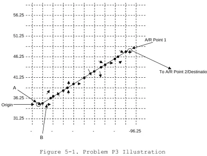
Figure 5-1. Problem P3 Illustration
In figure 5-1, the vector arrows within each grid box are
the wind vectors associated that with particular portion of
the grid. Note: the empty grid boxes also have associated
wind vectors, but are not shown in Figure 5-1. The calculated
bearing from the origin to aerial refueling point 1 is 44.196
degrees. Next, find the 99% max range speed the aircraft
should travel at. For simplicity sake, we shall assume this
to be 300 mi/hr for the first grid box we traverse, box A
(although in the actual algorithm, one should compute the 99%
max range speed based on aircraft weight and altitude). Next,
convert the origin and aerial refueling point 1 into mercator
points and we get:
A/R Point 1
Origin
To A/R Point 2/Destination
- - - -96.25
36.25 41.25 46.25 51.25 56.25
31.25
A
Origin = [W118, N38.6331]
Point 1 = [W96, N56.368]
Next, use the equation of a line: y= mx+b. First, find m (the
slope):
m = (y’-y)/(x’-x)=(-118+96)/(38.6331-56.3688061)=.8061
Now, plug in either the origin or point 1 to find b:
b = y-mx = 38.6331 - (.8061*-118) = 133.7567
Now, the equation of any point on the mercator map from the
origin to point 1 is:
y = .8061x + 133.7567
We know we need to find the following points on the line:
x: [-116.25 -113.75 -111.25 -108.75 -106.25 -103.75
-101.25 -98.75 -96.25]
y: [36.25 38.75 41.25 43.75 46.25 48.75]
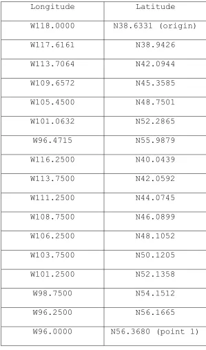
Plug the above points into the equation we found earlier and
Table 5-1. Example Mercator Grid Lines
Longitude Latitude
W118.0000 N38.6331 (origin)
W117.6161 N38.9426
W113.7064 N42.0944
W109.6572 N45.3585
W105.4500 N48.7501
W101.0632 N52.2865
W96.4715 N55.9879
W116.2500 N40.0439
W113.7500 N42.0592
W111.2500 N44.0745
W108.7500 N46.0899
W106.2500 N48.1052
W103.7500 N50.1205
W101.2500 N52.1358
W98.7500 N54.1512
W96.2500 N56.1665
W96.0000 N56.3680 (point 1)
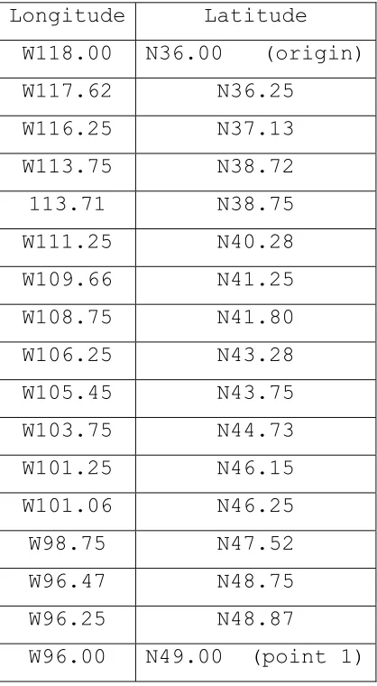
Now, we must convert these points back to spherical
coordinates, and sort them from the closest to farther points
Table 5-2. Example Spherical Grid Lines
Longitude Latitude W118.00 N36.00 (origin) W117.62 N36.25 W116.25 N37.13 W113.75 N38.72 113.71 N38.75 W111.25 N40.28 W109.66 N41.25 W108.75 N41.80 W106.25 N43.28 W105.45 N43.75 W103.75 N44.73 W101.25 N46.15 W101.06 N46.25 W98.75 N47.52 W96.47 N48.75 W96.25 N48.87 W96.00 N49.00 (point 1)
Now, assume the associated wind vector in box A is 35 mi/hr at
a direction of 120 degrees (0 degrees is due north). The
length of the segment in box A is simply the great circle
distance from the origin, (-118 36), to
(-117.62 36.25). This is 27.5 miles. The aircraft velocity
vector is:
x = 300*sin(44.196) = 209.13
The wind velocity vector is:
x’ = 35*sin(120) = 30.31
y’ = 35*cos(120) = -17.50
Now, we would like to keep our original velocity vector, so
taking the wind vector into account, we get:
x’’ = 209.13 + 30.31 = 239.44
y’’ = 215.09 – 17.50 = 197.59
Next, compare the new magnitude, x''2+y''2 = 310.44, to our
original velocity magnitude, 300. Since 310.44>300, this
route with wind present is going to take less effort than
without the wind present. Thus, to account for the wind, we
take the ratio of the original velocity to the wind factored
velocity and apply this to the distance and get:
÷ ×
(300 310.44) 27.5 = 26.57. Now, calculate the amount of fuel
used for a distance of 26.57 miles. Subtract this amount from
the original fuel allocation for the aircraft and then compute
the new 99% max range speed for the next grid box, B. Repeat
these steps to figure out the wind adjusted distance for grid
box B and then repeat for each successive grid box until
aerial refueling point 1 is reached. When aerial refueling
point 1 is reached, we will have a fuel cost for leg 1, and
then move onto the leg 2 and repeat all the aforementioned
steps. Repeat this procedure for all legs of the routing for
With the wind adjusted total fuel cost, one then just uses the
algorithm described in problem (P2) and keeps recomputing the
wind adjusted total fuel cost as aerial refueling points are
CHAPTER VI
ANALYSIS OF THE ALGORITHM
1 Aircraft
N Aerial Refuelings
Non-Instantaneous Refueling
Comparison of Algorithm vs Current Planning Tools
Currently, the U.S. Air Force uses the Combined
Mating and Ranging Planning System (CMARPS) to plan aerial
refueling missions. For the most part, this tool directly
routes any deploying aircraft onto their great circle routes
(provided no restricted airspace is infringed upon during this
route), thus, minimizing the distance traveled by that
aircraft. It then places any needed aerial refuelings on this
great circle route according to refueler and abort base
availability. The algorithms derived in this paper use a
safety stock of fuel to deal with emergency situations rather
than specifically looking at distances to abort bases. Due to
this fact, we will also examine the effect on total fuel
end of this chapter. The U.S. Air Force has provided 3 sample
missions they planned using CMARPS. The U.S. Air Force
mission details are in Tables 6-1, 6-2, 6-3, and 6-4. In all
scenarios, the deployment aircraft is a C-5 and the aerial
refueling aircraft are KC-10’s.
Table 6-1: Base Information.
Mission Origin Destination Aerial
Refuelings A/R Base 1 A/R Base 2 1 N39.133 W75.467 S31.933 E115.966 2 N38.266 W121.933 N13.583 E144.933 2 N38.266
W121.933 E115.966 S31.933 2 N38.266 W121.933 E144.933N13.583 3 N33.88 W117.258 N9.516 E44.083 2 N47.966 W97.40 N63.983 W22.60
Table 6-2: CMARPS Data Results.
Mission Offload #1 (lbs) Offload #2 (lbs) A/R Point 1 Beginning A/R Point 2 Beginning Total Fuel Consumption (lbs) 1 193,100 153,000 N50.233
W122.60
N21.50 E166.33
755,657
2 139,500 90,000 N32.66
W143.633 E166.483 N1.067 657,505 3 214,700 193,500 N45.033
W109.60
N66.366 W13.033
Table 6-3: CMARPS Fuel Consumption.
Mission C-5 Fuel Consumption
(lbs)
KC-10 #1 Fuel
Consumption (lbs) Consumption (lbs)KC-10 #2 Fuel
1 563,252 72,683 119,722
2 445,799 106,261 105,445
3 496,432 61,085 40,059
Table 6-4. Mission Parameters
Mission C-5 Cargo Weight (lbs) C-5 Initial Fuel (lbs) KC-10 #1 Initial Fuel (lbs) KC-10 #2 Initial Fuel (lbs)
1 100,000 267,150 310,000 330,000 2 100,000 267,150 260,000 260,000 3 190,000 114,150 330,000 280,000
Now, using the same input parameters given above, let us
examine the solution for each mission using the algorithm
derived in this paper. These results are shown in Tables 6-5
and 6-6.
Table 6-5: Algorithm Data Results.
Mission Offload #1 (lbs) Offload #2 (lbs) A/R Point 1 Beginning A/R Point 2 Beginning Total Fuel Consumption (lbs) 1 188,010 135,129 N48.18
W120.88
N14.74 E147.19
656,971
2 92,089 127,057 N26.35
W156.08 E146.04 N11.71 618,679 3 232,597 186,851 N43.37
W110.68
N65.64 W21.35
Table 6-6: Algorithm Fuel Consumption.
Mission C-5 Fuel Consumption
(lbs)
KC-10 #1 Fuel Consumption
(lbs)
KC-10 #2 Fuel Consumption
(lbs)
1 563,797 61,829 31,345
2 456,933 133,432 28,313
3 506,019 62,958 26,259
As one would expect, the fuel savings using the
algorithm described in this paper come from better placement
of the refueling aircraft (the KC-10’s). The C-5 burns more
fuel using the described algorithm than CMARPS due to the fact
that it is not possible for the C-5 to take a shorter route
than the one prescribed by CMARPS.
Table 6-7 and Figure 6-1 show the affect of varying the
reserve fuel requirement on the first mission. As one would
expect, more fuel held in reserve drives the total fuel
consumption higher as this forces the tanker aircraft to
travel greater distances during the mission.
Table 6-7: Effect of Reserve Fuel on Fuel Consumption (Mission 1).
Reserve Fuel Requirement (lbs) Total
Fuel Consumption (lbs)
Total Fuel Consumption 620000 630000 640000 650000 660000 670000 680000 690000 700000 710000 720000 730000
35000 50000 55000 60000 70000
Reserve Requirement (lbs)
To ta l F u e l C o n s um pt io n ( lbs )
Total Fuel Consumption
Figure 6-1: Reserve Fuel vs Safety Stock.
The overall performance of the algorithm holds up quite
well in these examples. In every case, it outperformed the
current method of mission planning. Table 6-8 shows the
actual comparisons via mission. On average, the algorithm
saved 6.96% in fuel consumption on a given mission.
Table 6-8: Comparison.
Mission Algorithm Fuel Consumption (lbs) CMARPS Fuel Consumption (lbs) Fuel Savings (lbs) Percentage of Savings
1 656,971 755,657 98,686 13.06%
2 618,679 657,505 38,826 5.91%
Observation of an Additional Decision Variable
When running through the scenarios described above, it is
apparent that the 2 decisions variables are:
1. What point to refuel at?
2. How much to offload at that point?
However, if we look at the fuel used and offloaded by each
KC-10 above, we can come up with another decision variable that
could possibly save fuel and money:
3. How much fuel to initially have in each KC-10?
Looking at our results, it is clear that in all cases, we can
start with less fuel in the refueling aircraft. Let’s assume
that 30,000 pounds is the reserve requirement for the KC-10’s.
Therefore, the refueling aircraft must land with this amount
of fuel. Table 6-9 shows the excess fuel we are carrying for
Table 6-9: KC-10 Fuel Utilization.
Mission KC-10 Initial
Fuel ConsumedFuel OffloadedFuel Fuel Left 1 310,000 61,829 188,010 60,161 1
2 330,000 31,345 135,129 163,525 1 260,000 133,432 92,089 34,479 2
2 260,000 28,313 127,057 104,630 1 330,000 62,958 232,597 34,445 3
2 280,000 26,259 186,851 66,890
Table 6-10: New Initial KC-10 Fuel Allocations.
Mission KC-10 Initial
Fuel RemainingFuel Excess Fuel Initial New
1 310,000 60,161 30,161 277,050 1
2 330,000 163,525 133,525 195,800 1 260,000 34,479 4,479 254,400 2
2 260,000 104,630 74,630 185,000 1 330,000 34,445 4,445 325,500 3
2 280,000 66,890 36,890 241,900
Table 6-11 shows the results for each mission using the new
initial fuel for the KC-10’s under the enhanced algorithm
column. This enhancement slightly increases efficiency and
boosts the fuel savings to 7.28% from the current system.
Table 6-11: Enhanced Algorithm Comparison.
Mission Algorithm Fuel Consumption (lbs) CMARPS Fuel Consumption (lbs) Enhanced Algorithm Fuel Consumption (lbs) Fuel Savings (lbs) Percentage of Savings
1 656,971 755,657 653,451 102,206 13.52% 2 618,679 657,505 617,130 40,375 6.14%
If we were to assume that a gallon of jet fuel costs the
U.S. government $1.50 per gallon and one gallon is 6.8 pounds,
the savings from using this algorithm on these three missions
alone would be over $32,274. Assuming that these missions are
a fraction of the daily workload for the Air Force, the