Computer Simulation of Chemical Reactions in Porous Materials

ABSTRACT

TURNER, CHRISTOFFER HEATH. Computer Simulation of Chemical Reactions in Porous Materials. (Under the direction of Keith E. Gubbins.)

Understanding reactions in nanoporous materials from a purely experimental perspective is a difficult task. Measuring the chemical composition of a reacting system within a catalytic material is usually only accomplished through indirect methods, and it is usually impossible to distinguish between true chemical equilibrium and metastable states. In addition,

measuring molecular orientation or distribution profiles within porous systems is not easily accomplished. However, molecular simulation techniques are well-suited to these

challenges. With appropriate simulation techniques and realistic molecular models, it is possible to validate the dominant physical and chemical forces controlling nanoscale reactivity. Novel nanostructured catalysts and supports can be designed, optimized, and tested using high-performance computing and advanced modeling techniques in order to guide the search for next-generation catalysts - setting new targets for the materials synthesis community.

We have simulated the conversion of several different equilibrium-limited reactions within microporous carbons and we find that the pore size, pore geometry, and surface chemistry are important factors for determining the reaction yield. The equilibrium-limited reactions that we have modeled include nitric oxide dimerization, ammonia synthesis, and the esterification of acetic acid, all of which show yield enhancements within microporous carbons. In

ethyl acetate within carbon micropores demonstrates an efficient method for product recovery.

COMPUTER SIMULATION OF CHEMICAL REACTIONS IN POROUS MATERIALS

by

CHRISTOFFER HEATH TURNER

A thesis submitted to the Graduate Faculty of North Carolina State University in partial

fulfillment of the requirements for the Degree of Doctor of Philosophy

CHEMICAL ENGINEERING

Raleigh 2002

APPROVED BY:

Keith E. Gubbins, Chair Carol K. Hall

BIOGRAPHY

Heath Turner was born in Birmingham, Alabama on November 15, 1973 to parents Gary and Cheryl Turner. Heath was raised in Birmingham, along with an older brother Bart and a younger sister Tiffany, and graduated from Mountain Brook High School in 1992.

After graduating from high school, Heath attended Auburn University in Auburn,

ACKNOWLEDGMENTS

I would like to begin by thanking my wife, Christy, for her support, patience, and encouragement during my education. She has made my life enjoyable and fun, even when research wears me down. Most importantly, she has kept me well- fed day and night.

My parents also deserve much appreciation for their help. They have emphasized the importance of learning throughout my life, and have helped support me financially and otherwise, while I have been in school. I value my education second only to the things they have taught me.

My experience at NC State would not have been nearly as enjoyable or as enlightening without the diverse group of people that I have had the privilege to work with: Lev Gelb, Simon McGrother, Karl Travis, Ravi Radhakrishnan, Ken Thomson, Sandra Gavalda, Jorge Pikunic, Philip Llewellyn, Martin Lisal, John Brennan, Lauriane Scanu, Flor Siperstein, Alberto Striolo, Henry Bock, Coray Colina, Francisco Hung, Supriyo

I would also like to thank several people outside of my research group that I have been able to work with. Jerry Whitten has given me a great deal of help and advice with quantum mechanical calculations. Also, I would like to thank Karl Johnson for the thoughtful criticisms and suggestions throughout my research. I have also been fortunate enough to discuss the experimental work related to my project with Katsumi Kaneko, Malgorzata Sliwinska-Bartkowiak, and John Yates. Additionally, I would like to thank Sandeep Tripathi and Walter Chapman for sharing their insights and knowledge.

Finally, I would like to thank my advisor, Keith Gubbins, and the rest of my thesis

committee for their help and guidance. Keith has a talent for balancing many tasks, while at the same time maintaining a high standard of quality. He has done a great job of exposing me to a broad range of research, and he has provided me with many

TABLE OF CONTENTS

LIST OF TABLES vii

LIST OF FIGURES viii

1. INTRODUCTION 1

1.1 Motivation 1

1.2 Defining the Research Agenda 4

1.3 Available Simulation Methods 6

1.4 Simulating Chemical Reaction Equilibria 9

1.5 Simulating Chemical Reaction Kinetics 18

1.6 Overview of our Work 28

References 30

2. NITRIC OXIDE DIMERIZATION 36

2.1 Introduction 36

2.2 Simulation Methods 39

2.3 Simulation Models 44

2.4 Results and Discussion 48

2.5 Conclusions 56

References 59

3. AMMONIA SYNTHESIS 76

3.1 Introduction 76

3.3 Simulation Models 83

3.4 Results and Discussion 88

3.5 Conclusions 100

References 103

4. ESTERIFICATION OF ACETIC ACID 122

4.1 Introduction 122

4.2 Simulation Methods 126

4.3 Simulation Models 130

4.4 Simulation Results 136

4.5 Conclusions 145

References 147

5. EFFECT OF CONFINEMENT ON REACTION KINETICS 162

5.1 Introduction 162

5.2 Methodology 165

5.3 Verification of the TS-RxMC Method 176

5.4 Effects of Strong Intermolecular Forces and Confinement 183

5.5 Discussion and Conclusions 189

References 193

6. CONCLUSIONS 206

6.1 Reaction Equilibria 206

LIST OF TABLES

CHAPTER 2

2.1 Summary of Lennard-Jones parameters 45

2.2 Conversion of nitric oxide dimerization in the bulk gas phase 54

CHAPTER 3 3.1 Summary of intermolecular potential parameters 84

3.2 Summary of potential parameters for –COOH sites 86

3.3 Adsorbate density within slit-pores at a pressure of 100 bar 91

3.4 Selectivity of N2 over H2 in a 0.83 nm wide pore at 573 K 93

3.5 Ammonia mole fraction corresponding to Figure 3.11 94

CHAPTER 4 4.1 Summary of intermolecular potential parameters 131

4.2 Coefficients for the intramolecular potentials 132

4.3 Rotation and vibrational constants used in the partition functions 134

4.4 Experimental yield of ethyl acetate in activated carbon 141

4.5 Yield of ethyl acetate at 473.15 K and 523.15 K 144

CHAPTER 5 5.1 Intermolecular parameters for the 2HI↔

( )

LIST OF FIGURES

CHAPTER 1

1.1 Molecular Simulation Scales 35

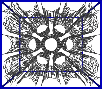
CHAPTER 2 2.1 Snapshot of the (10,10) carbon nanotube bundle, without defects 62

2.2 Snapshot of the (10,10) carbon nanotube bundle, with 5% defects 63

2.3 Conversion of NO dimerization in the bulk saturated liquid 64

2.4 Conversion of NO dimerization within slit-shaped carbon pores 65

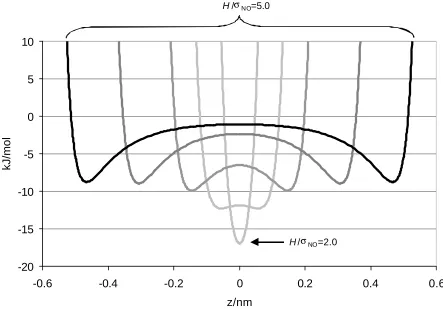
2.5 Potential energy profile of NO within slit-pores 66

2.6 Density profiles of NO and (NO)2 in the slit pore, H/σNO = 5.50 67

2.7 Density profiles of NO and (NO)2 in the slit-pore, H/σNO = 2.50 68

2.8 Effect of bulk gas pressure on the adsorption and reaction equilibrium 69 2.9 Conversion of NO dimerization within slit-shaped pores from DFT 70

2.10 Conversion of NO dimerization in the perfect (10,10) nanotubes 71

2.11 Snapshots in (10,10) nanotubes at different loadings 72

2.12 Snapshots in (10,10) nanotubes with different separation distances 73

2.13 Conversion of NO dimerization in the defective (10,10) nanotubes 74

2.14 Adsorbate density within the (10,10) nanotubes during reaction 75

CHAPTER 3 3.1 Structure of the –COOH activation site used in simulation 105

3.3 Radial distribution function of the coconut shell carbon model 107

3.4 Hexagonal packing of the carbon nanotubes used in simulation 108

3.5 Mole fraction of NH3 for the bulk phase reaction 109

3.6 Mole fraction of NH3 for the bulk phase reaction with inert gases 110

3.7 Nitrogen adsorption isotherm at 303 K in activated carbon fibers 111

3.8 Hydrogen adsorption isotherm at 293 K in AX21 carbon 112

3.9 Simulations of ammonia synthesis in carbon slit-pores 113

3.10 Conversion of ammonia synthesis at 573 K and 100 bar 114

3.11 Ammonia synthesis in carbon slit-pores with varying N2:H2 ratios 115

3.12 Pore size distribution of the coconut shell carbon model 116

3.13 Snapshot of a carbon slit-pore, chemically activated by –COOH 117

3.14 Conversion of NH3 in chemically activated slit-pores (H=1.6 nm) 118

3.15 Conversion of NH3 in chemically activated slit-pores (H=1.0 nm) 119

3.16 Snapshot of ammonia synthesis in a chemically activated slit-pore 120

3.17 Conversion of NH3 in carbon nanotube bundles 121

CHAPTER 4 4.1 Conversion of acetic acid to ethyl acetate in the bulk gas phase 151

4.2 Smooth slit-pore and activated slit-pore models 152

4.3 Conversion of acetic acid to ethyl acetate in 90 mole % CO2 153

4.4 Snapshot of esterification in 90% CO2 at 450 K 154

4.5 Snapshot of esterification in 90% CO2 at 360 K 155

4.7 Mole fraction of ethyl acetate in activated and unactivated carbon

slit-pores 157

4.8 Total mole fraction of ethyl acetate in the two-phase system (bulk + pore) composed of a bulk gas phase and a carbon slit-pore (unactivated) 158

4.9 Total mole fraction of ethyl acetate in the two-phase system (bulk + pore) composed of a bulk gas phase and a carbon slit-pore (activated) 159

4.10 Total conversion of acetic acid in a pore width H=2.0 nm 160

4.11 Snapshot of esterification within the activated pore 161

CHAPTER 5 5.1 Structure of the

( )

5.2 TS-RxMC simulations for HI decomposition at 573.15 K 196

5.3 TS-RxMC simulations for HI decomposition at 594.55 K 197

5.4 Comparison of simulations with Eckert and Boudart 198

5.5 Equilibrium constant of the HI decomposition reaction at 573.15 K 199

5.6 Effect of adjusting the activation barrier for H2 exchange reaction 200

5.7 Effect of adjusting the activation barrier for HI decomposition 201

5.8 TS-RxMC simulations of HI decomposition in inert solvents 202

5.9 TS-RxMC simulations of HI decomposition in carbon slit-pores 203

5.10 HI decomposition rate versus density in the bulk and in the pore 204

CHAPTER 1

Introduction

1.1 Motivation

The research that we present is motivated by the need to understand reactions that are altered by strong intermolecular forces, such as reactions at high pressures, reactions in inert

solvents, and most importantly, reactions occurring within microporous materials. There is a great deal of interest from a practical standpoint to understand the molecular level

interactions and forces that dictate macroscopic level phenomena such as reactant selectivity, reaction conversion, and the kinetic properties of reacting systems. Knowledgeable design of porous catalysts and catalyst support materials can result in increased conversions, higher reaction rates, higher product selectivity, and many derivative environmental benefits.

Another recent contribution [3] in this area has examined the effects of geometric

confinement on the creation of self-assembled monolayers (SAMs) on gold surfaces. During a process that the authors term "nanografting", it is found that the development of thiol-derived SAMs are favored in the geometrically confined space between an atomic fo rce microscopy (AFM) tip and a gold surface. It is suggested that spatial confinement between the surface and the AFM tip alters the mechanism and kinetics of the surface reactions by preventing alternative reaction pathways and stabilizing particular transition states or reaction intermediates. In addition, the authors find that the SAMs created at the tip of the AFM tend to be free of defects, in contrast to SAMs formed in otherwise unconstrained environments.

In another related area, Brunet has recently reviewed [4] applications of using confinement to determine the stereochemical outcome of a reaction through space constriction and molecular close contact, thus providing an alternative method for enantiomeric separation. In this work, Brunet reviews several potential methodologies for confinement-induced asymmetric

induction of chemical reactions. One of these techniques is called molecular imprinting, which strives to imprint orifices within polymeric matrices having structures that mimic the transition state of enantioselective processes. This potentially lowers the activation barrier for a selected enantiomer and increases the selectivity. Another route to asymmetric

induction is the development of temporary microscopic chiral molecular capsules or vessels with a complementary structure specific to the reactants [5,6]. It is envisioned that

auxiliaries and pro-chiral molecules within cationic pores of zeolites in order to induce diastereoselectivity. It has been shown that confinement within the orifices of zeolites can dramatically enhance the transfer of chirality as compared to an unconfined system [7]. The last methodology reviewed [4] is the possibility of constructing hybrid organic- inorganic materials, and using the cavities within these frameworks as catalytic points for

enantioselective reactions. The performance of these hybrid materials for enantioselective catalysis is still being evaluated.

The above examples clearly demonstrate the importance of understanding the phenomena contributing to reactivity in microscopically constrained environments. We have attempted to contribute to this area by expanding the understanding of chemical reaction equilibria and chemical reaction kinetics using molecular- level simulations. The next section will explain the specific focus that we have adopted for our work.

1.2 Defining the Research Agenda

The above examples demonstrate the significant effects and potential benefits for conducting chemical reactions in confined systems. We have attempted to contribute to this broad area, by again addressing the following question: how does the surrounding environment, and in particular, confinement within porous materials, influence a chemical reaction? In order to differentiate our investigation from previous studies, it is helpful to identify the most important questions that will define the scope of our project:

(a) How does the equilibrium conversion of a reaction within a porous material compare to the same reaction in the bulk gas phase, at a given temperature and pressure of the bulk phase?

(b) Does the selectivity of reactant and product molecules in a pore affect the conversion of a reaction?

(d) Can the surface chemistry within a pore be modified in order to shift the equilibrium of the reacting system?

(e) How is the heat of reaction affected within a porous material as compared to the bulk gas phase?

(f) How are reaction rates influenced by the surrounding environment, such as inert solvents or confinement within porous materials?

(g) Can the geometry of a micropore affect the kinetics of a chemical reaction?

Since we are primarily interested in learning about the fundamental nature of reactions within porous materials and other non- ideal environments, we start with simple reactions within well-defined pore structures having simple surface chemistries. While this research is intended to influence and shape the understanding of realistic reacting systems, an

experimental investigation of this nature can produce ambiguous results. In experimental studies there are inevitable complications arising from competing side reactions, long- lived metastable states, uncertainties arising from the micropore characterization, uncertainties in determining the me an compositions and composition profiles in the pores, etc. Simulation methods allow precise control of these variables and determination of the true

1.3 Available Simulation Methods

Once it is apparent that simulations are best suited to this type of investigation, it is then necessary to decide which types of simulations to employ. The answers to the previous questions can be investigated from several different perspectives and length scales: quantum mechanical simulations, Monte Carlo (MC) simulations, molecular dynamics (MD), finite element simulations, all the way up to continuum approximations. There are unfortunate tradeoffs between accuracy and efficiency as the focus shifts from the quantum mechanical level all the way up to the continuum level. This is shown quantitatively in Figure 1.1, which illustrates the length and time scales accessible with each computational method. This Figure was constructed assuming that computations are performed for a maximum of one week on the Blue Horizon (SP3) supercomputer located at the San Diego Supercomputer Center (SDSC), which has a maximum speed of 1.728 Tflops (1 Tflop = 1×1012 floating point operations per second). As more approximations are introduced into the computational methods, the length and time scales accessible grow exponentially.

structure of the atoms and molecules involved, and must be studied with quantum mechanical techniques.

However, in supported catalysis we anticipate a further significant effect of confinement on the reaction rate, due to the finite size and reduced dimensionality of the adsorbed phase, and to the strong interactions of the reacting species with the pore walls. We refer to these latter interactions (repulsion, dispersion, electrostatic, etc.) as "physical" forces to distinguish them from the chemical interactions with the catalyst itself. For these reasons, we have elected to use semi-classical Monte Carlo methods. This level of approximation allows us to simulate realistic molecular systems composed of millions of molecules, yet still accurately capture the physical effects on chemical reactions which we wish to understand.

By performing Monte Carlo simulations and accumulating statistical averages of the system, we can accurately measure quantities such as the number of molecules of various species adsorbed in a pore, the heats of adsorption, the density, the molecular arrangement within the pores, etc. We begin by assuming that a given system maintains a Boltzmann distribution of states. Then by applying the rules of statistical mechanics, an arbitrary observable system property 〈A〉 may be calculated according to the following equation:

( )

[

]

( )

( )

[

]

∫

∫

= _{N N}

In Eq. (1.1), β=1/kBT is the reciprocal of the Boltzmann constant times the temperature, and U is the configurational energy of the system, which depends on the coordinates,

rN=r1r2...rN, of the N molecules in the system. Although it is usually not possible to solve Eq. (1.1) analytically, it can be statistically approximated as an average over randomly generated system configurations, according to:

( )

[

( )

]

( )

[

]

∑

∑

A (1.2)

By generating many different system configurations, τ, and sampling the average va lue of the property 〈A〉 at each of these configurations, an accurate estimate of the integral, and thus the equilibrium value of A can be obtained. However, in practice it turns out that only a small number of randomly generated configurations make non-negligible contributions to the average, due to highly energetic overlaps encountered between the molecules in the system. Thus, the utility of the Monte Carlo method hinges on various algorithms to efficiently sample the most probable configurations for a given system.

explore the most significant contributions to ensemble averages. The following sections give brief reviews of the development and application of Monte Carlo methods for predicting chemical reaction equilibria and kinetics in environments where intermolecular interactions are significant. For our applications, the simulations must be flexible enough to allow us to look at reactions between individual molecules, reactions occurring in multiple phases, and reactions in which the number of moles changes.

1.4 Simulating Chemical Reaction Equilibria

1.4.1 Available Methods

While the bond breaking and bond formations associated with forward and reverse reaction steps are statistically inaccessible in a typical Monte Carlo search, in 1981 Coker and Watts devised one of the first simulation methods which was able to deal with this challenge [9,10]. Their technique was based on grand canonical Monte Carlo (constant chemical potential, volume, and temperature), but was modified to directly sample forward and reverse reaction steps. Thus the high-energy process of bond breaking and bond formation is circumvented by directly simulating the equilibrium between the reactants and the final products. The total number of molecules was held fixed in their simulations, but the identities of the individual molecules were allowed to vary. However, in order to sample these identity cha nges, the chemical potential differences between the two species had to be specified. Coker and Watts used their method to simulate the equilibrium conversion of the reaction:

Their simulated mole fractions were found to agree closely with experimental measurements, within the small temperature range that they investigated. However, in addition to requiring the chemical potentials as a necessary input, their method was restricted to chemical

reactions that preserve the total number of moles in the system.

In 1988, Kofke and Glandt proposed an improved simulation technique to model both reaction equilibria and phase equilibria [11]. They termed their new method the semigrand canonical ensemble MC method, and used it to study the same reaction as Coker and Watts, Eq. (1.3). This method was more versatile and corrected some of the errors in the method of Coker and Watts, such as mistakes in the equilibrium constant, the acceptance criteria, and an incorrect form of Widom's particle insertion method [12]. The semigrand ensemble samples forward and reverse reactions by using the ratios of the component fugacities to a reference fugacity in the acceptance criterion, instead of using chemical potentials. While this method was an improvement over the method of Coker and Watts, its application was still restricted to reactions in which the number of moles remained fixed.

N2 + O2↔ 2NO (1.4)

Shaw's method was a significant improvement over previous methods, primarily because simulations could be performed in the more convenient isothermal- isobaric ensemble. Chemical equilibrium along with other thermodynamic quantities could be measured at constant pressure, temperature and total number of atoms, which allowed more natural comparison with experiments. In the NatomsPT ensemble, the acceptance criteria for the forward and reverse reaction steps involves only the ideal gas partition functions for the reaction components, and the method can, in principle, accommodate reactions tha t involve a change in the number of moles. However, due to its cumbersome nature, there have been no applications of this method to reactions that change in mole number.

to accommodate particles with multiple binding sites that form higher order complexes. Their primary focus was studying antigen-antibody interactions. While the ABMC method efficiently samples the important regions of phase space, the calculations necessary for the biasing can become quite complicated.

Tsangaris and de Pablo developed a method that they named bond-bias Monte Carlo

(BBMC) [17]. Similar to the ABMC method, their technique also biased Monte Carlo moves into areas of phase space significant to bond breaking and bond formation. The BBMC technique therefore avoids the high-energy activation barrier usually associated with strong associa tions and efficiently samples phase space. With BBMC simulations, Tsangaris and de Pablo studied the phase equilibria and energetics of acetic acid dimerization, Eq. (1.5), and achieved close agreement with experimental data and theoretical predictions.

2CH3COOH ↔ CH3C(OHO)2CCH3 (1.5)

Another Monte Carlo method was developed by Shew and Mills to simulate systems that involve high energy barrier crossings, such as chemical reactions [18-20]. Their method was named the subspace sampling method (SSM), and it works by partitioning configuration space into regions which are separated by potential energy barriers or by different

hamiltonians. While they began with studies in one dimension [18,20], they later applied their method to simulate the thermodynamic and structural properties of a weak electrolyte solution in three-dimensional space [19]. Although reasonable results can be obtained with this method, an adjustable simulation parameter must be optimized in order to achieve convergence rates comparable with other methods.

The most powerful and flexible technique for simulating molecular reaction equilibria to date was developed simultaneously by two separate groups, Smith and Triska [21] and Johnson et al. [22], which we collectively refer to throughout this work as the Reactive Monte Carlo (RxMC) simulation method. The two methods are similar to the one developed by Shaw [13], except that the method can be easily applied to reactions that change in mole number. Additionally, multiple simultaneous reactions can easily be studied, as can reactions in multiple phases, and reactions within porous materials. Both renditions of this method [21,22] simulate reaction equilibria through trial attempts of complete forward and reverse reaction steps (in addition to the traditional Metropolis Monte Carlo moves), while

conserving the total number of atoms in the system. Although the simulation technique of the two groups is virtually identical, the acceptance probability for a reaction step is

acceptance probability for a reaction step is formulated by Smith and Triska in terms of the Gibbs free energy of reaction. Consequently, the two methods are interchangeable, as the Gibbs free energy of reaction can be easily formulated in terms of the molecular partition functions.

1.4.2 Recent Applications of Reactive Monte Carlo

Aside from the research presented in the following chapters of this work, there have only been a few applications of the RxMC simulation technique. The first application of the RxMC method to a realistic molecular reaction was performed by Johnson et al. [22] in order to study the dimerization of nitric oxide in both the gas and liquid phases:

2NO ↔ (NO)2 (1.6)

Subsequently, Lisal et al. published a series of papers applying the RxMC method (therein referred to as the reaction ensemble method) to realistic molecular reactions [25-27] and to complex phase equilibria [28,29]. Although chemical reactions are not considered in references [28] and [29], phase equilibrium is treated as a special case of chemical

equilibrium. According to this treatment, the Gibbs ensemble technique is combined with the RxMC moves in order to predict accurate phase behavior of complex binary mixtures involving water, methanol, ethanol, carbon dioxide, isobutene, MTBE, and n-butane.

The first realistic reaction that this group studied was the equilibrium of the bromine-chlorine system, Eq. (1.3). This reaction has been modeled previously using other simulation

methods, such as that of Coker and Watts [9,10] for a study of the liquid phase conversion and by Kofke and Glandt [11] for a study of simultaneous reaction and phase equilibrium. Lisal et al. [25] expanded upon the work of these previous studies to map out the complete simultaneous reaction and phase equilibrium diagram of the bromine-chlorine system. Their agreement with previous simulation and experimental results was good, and they were able to contribute additional information about this system where experimental data is inaccessible (due to the chemical instability of the system).

The second application of RxMC simulations by Lisal et al. [27] was to high temperature chemically reacting plasmas, in which the ionization reactions of helium were modeled:

He+↔ He++ + e- (1.8)

These simultaneously occurring ionization reactions were studied at high temperatures (up to 100,000 K) and high pressures (10, 100, and 400 MPa), and the equilibrium results were compared with predictions from the classical Debye-Hückel (DH) macroscopic model [30]. The authors calculate the composition of the plasma, molar enthalpies, molar volumes, molar heat capacities, and coefficients of cubic expansion for this system. The predictions from the DH theory tend to slightly underpredict the amount of ionization in the plasma as the

pressure is increased. Additionally, the DH predictions tend to be least accurate when calculating the coefficient of cubic expansion and the molar heat capacity, by up to 40% at the highest pressure (400 MPa).

The most recent contribution from Lisal et al. [26], is an extension of the RxMC method to constant enthalpy and constant internal energy simulations. The utility of this approach is demonstrated by simulating the conversion of ammonia synthesis within an adiabatic plug flow reactor. The enthalpy corresponding to the inlet composition, a stoichiometric feed of H2 and N2, is first calculated. Then, this value is used to perform a RxMC simulation at constant enthalpy and pressure to determine the exit composition and temperature.

Brennan and Rice have used RxMC to study the shock properties of liquid NO and liquid N2 [31]. RxMC simulations were carried out at high pressures (2-90 GPa) and high

Excellent agreement was found with experimental measurements at these conditions. The RxMC method shows great promise in the development of novel energetic materials, in testing current detonation theories, and in furthering our understanding of materials under shock.

Reactive Monte Carlo simulations have also been used to study [32] the ammonia synthesis reaction at conditions characteristic of the deep atmosphere of Jupiter (temperatures between 500 and 2300 K and at pressures up to 10,000 bar):

N2 + 3H2↔ 2NH3 (1.9)

In order to compare with experiments, simulations were also performed at 573 K and 873 K and in pressure ranges where experimental data is available (100 to 1,000 bar), and close agreement was found with the available data. We have performed similar simulations of the ammonia synthesis reaction, which will be presented later in Chapter 3 of this work.

2A ↔ B (1.10)

They use the Reactive Monte Carlo method for their simulations, but they arbitrarily allow the ideal gas contribution of the equilibrium constant to vary with respect to distance from the pore walls. This is a quantity that we have not allowed to vary in our work for a given reaction. They find that the bulk phase composition favors the creation of B molecules at higher densities, according to LeChatlier's Principle, as the forward reaction results in a reduction in the number of moles. This effect is magnified within the pore phase, as the confinement tends to show an increased conversion due to preferential solvation within the adsorptive pore (in cases when the equilibrium constant is held fixed). When the equilibrium constant is allowed to vary, the confinement within the pore has a mixed effect on the

reaction conversion, depending on the relative effects of the adsorption and the surface-mediated changes allowed in the equilibrium constant.

1.5 Simulating Chemical Reaction Kinetics

1.5.1 Available Methods

help give some perspective to the method that we have developed [34] and to the systems and forces that we are able to study with our method, which will be discussed in Chapter 5.

A. Continuum Methods

Starting with general expressions used for reaction rate constants at the highest level of approximation should give justification for the more fundamental research performed on the smaller length scales, such as our own. As an example, the rate (rA) for an elementary binary chemical reaction, A+B→C, can be expressed in terms of the reactant concentrations and a rate constant (kobs), and this rate “constant” is typically assumed to only depend on the temperature according to Eq. (1.12):

[ ]

_{[ ][ ]}

obs

A k

dt d

r = = (1.11)

( )

(

)

k_obs = exp _a (1.12)

In Eq. (1.11) and (1.12) kobs is the observed rate constant, where brackets denote the concentration of each species, t is time, A is the preexponential factor, Ea is the activation energy, and R is the gas constant. These two expression can be easily incorporated into engineering design equations for stirred-tank reactors, plug flow reactors, batch, semi-batch, etc. in order to describe the spatial or temporal rate of a chemical reaction.

the surrounding environment, the solvent, or the catalyst change. In order to quantify the change of a rate constant with respect to the environment, it is imperative to incorporate more details into the model than the simple temperature-dependent Arrhenius expression shown in Eq. (1.12). For example, additional expressions, such as Eq. (1.13) are available [35,36] which are able to roughly model the pressure dependence of rate constants:

RT V P

k_obs −∆ ≠

=    

 

∂ ∂ln

(1.13)

B. Classical Simulations

In order to more accurately predict the rate constant in non- ideal environments, it is

necessary to increase the amount of detail in the model. Within the context of transition state theory (TST) [37,39], the interactions with the environment can be accounted for in

simulation by calculating the free energy of solvation (∆Gsol≠ ) of a reaction. The free energy of solvation can then be added to the free energy of activation for the reaction in the ideal gas phase (∆G_gas≠ ) in order to account for the overall free energy of activation in the solvent (or other medium). The resulting expression for the rate constant is shown below, and reflects the strong dependence on the free energy of activation, ∆G≠, where ∆G≠= ∆G_sol≠ + ∆G_gas≠ :

(

)

h T k

k B _B

obs

≠

∆ −

=κ exp (1.14)

In the equation above, κ is the transmission coefficient, h is Plank’s constant, and kB is the Boltzmann constant. The transmission coefficient (κ) accounts for any recrossing of the activation barrier, and will have a value of less than one if recrossing is significant.

quantum mechanically, as with self-consistent reaction field (SCRF) methods. If the

molecular details of the solvent are included, which may be important for hydrogen bonding systems or other systems that have specific interactions, Monte Carlo or molecular dynamics simulations can be used to calculate the free energies in such molecular fluids.

Other solvation methods are also available within classical MC and MD simulations, which accumulate the probability of observing the extent of a predefined reaction coordinate. For instance, in the dissociation of HCl, the statistical elongation of the H-Cl bond distance in a simulation can be related to the free energy of dissociation in different environments. However, unless the potential energy associated with changes in the reaction coordinate is small (<5kBT), biasing methods such as umbrella sampling [43] must be used to accumulate accurate statistics.

Another approach on this same leve l of molecular detail is the free energy perturbation (FEP) method [44]. This method relates the change in free energy ∆G between two different systems A and B in terms of potential energy differences (δUA→B), as shown in Eq. (1.15), where the brackets denote ensemble averages.

(

)

(

)

G → =− _B − _{A→B B}

∆ ln δ (1.15)

assigned as the transition state for the reaction, and the free energy change for the formation of the transition state can be computed in a variety of non-ideal environments. If the two states (A and B) are not similar, then the convergence of the method will be slow. To avoid slow convergence, the transformation between the reactants and the transition state can be discretized into intermediate structures between the two states. The free energy difference of each incremental step can then be calculated in simulation and summed to give the total change in free energy from state A to state B.

trajectories. The reaction path ensemble can explicitly account for external forces, such as solvation effects, in identifying the transition state structure for a reaction. Further review and application of these two methods are discussed by Frenkel and Smit [43]. Quantum mechanical analogues of the time correlation technique also exist [50,51].

There are several ways to refine the rate constants determined from the above equilibrium solvation methods. First of all, corrections can be included to account for dynamic collision effects or frictional effects that might alter the rate constant. These effects are not

specifically included in the equilibrium solvation methods, but can be approximated separately and absorbed into the transmission coefficient, κ, shown in Eq. (1.14). The analytical theory of Kramers [52,53] and the transmission coefficient of Grote and Hynes [54] are fairly well established for accommodating these effects. A discussion of these methods and others for approximating the transmission coefficient is presented by Ruiz-Montero et al. [55]. Also, since external interactions can affect the free energy of activation, there is a form of transition state theory that varies the definition of the activated

configuration (i.e., transition state species) in order to minimize the rate constant. This widely-accepted approach, called variational transition state theory (VTST) [56-59], tends to give more accurate values of the rate constant.

C. Quantum Mechanical Simulations

While the methods described in the previous section are primarily classical methods, many of the molecular quantities and parameters used in these methods are taken directly from

quantum mechanical simulations. The quantum mechanical simulations are performed on a much smaller length scale, which limits the size and time scale of the simulations to a few hundred atoms and to a few picoseconds, but detailed information about the transition state geometry, quantum mechanical tunneling, energy barriers, etc. can all be calculated. This is extremely important to the calculation of rate constants since this type of information is either difficult or impossible to measure with experiments.

Both ab initio methods and density functional theory (DFT) methods are capable of

generating potential energy surfaces (PES), which are routinely used as input in classical MC and MD simulations for calculating rate constants. The calculation of a PES is usually attempted in order to identify a transition state species, which is defined to correspond to the maximum in the free energy during the course of a reaction. The observation of the

transition state is identified, the necessary parameters such as the activation energy and the transition state geometry can be calculated.

In addition to developing PES's, several quantum mechanical methods, similar to the

classical methods described above, are available for estimating rate constants in the presence of external interactions. For instance, Miller et al. [50,51] have developed a quantum

mechanical analog for implementing the time correlation function approach for calculating rate constants. Additionally, there is the quantized version of variation TST, which is reviewed by Truhlar et al. [61] and applications of which are demonstrated in ref. [62,63]. This is similar to the classical version, which varies the definition of the dividing surface to minimize the rate constant. Also, there is a path integral formulation of quantum TST [64], which can be applied to reactions in solution and has been reviewed by Voth [65,66]. Applications of these methods as well as other quantum mechanical approaches to reaction rates can be found in the ref. [61]. In order to refine predictions of rate constants, there is a quantum mechanical analog of the classical Kramers and Grote-Hynes theories, which was first derived by Wolynes [67], and can account for quantum mechanical tunneling through the activation barrier or non-classical reflection above the barrier.

Probably one of the most recent and most popular quantum mechanical methods for calculating rate constants in the presence of surrounding molecules is called the

between this method and other quantum mechanical methods is that a special technique is used to propagate the molecular orbitals. Instead of reoptimizing the orbitals at each step, the orbitals are assigned a fictitious mass and propogated along with the atomic nuclei. This maintains the orbitals on the ground-state (Born-Oppenheimer) surface in an efficient way and reduces the computational demands of the method. The main drawback of the Car-Parrinello method is that it is still limited to small systems (of the order of 100 atoms), similar to other quantum mechanical methods. Applications of this method to reactions in solution, at surfaces, and for biological processes have been recently reviewed by Trout [69].

1.5.2 Integration of RxMC Simulations with Transition State Theory

Since we are primarily concerned with the physical interactions, such as confinement within porous materials, on chemical reaction kinetics, we have primarily used semi-classical methods to study rate constants. Although we have adopted a semi-classical simulation approach to our project, much of the information about the transition state and the activation energy for the reaction must be gathered from separate studies at the quantum mechanical level.

order of 106 atoms, and achieve close agreement where experimental comparison is available. Our methodology is described in detail in Chapter 5, as well as applications of this method to the kinetics of hydrogen iodide decomposition in a variety of non- ideal environments.

1.6 Overview of Our Work

1.6.1 Equilibrium Studies

From the survey given in Section 1.4, it is clear that little work on confined reactions has been reported. In the following chapters, we will present our simulation results for several realistic systems. While the work of Borówko and Zagórski [33] and other contributions [70 -77] give some insight into confined chemical reactions by studying simple, idealized

reactions and associations, we have chosen to model more realistic reactions using detailed micropore models. We have chosen to model several systems, which we believe explore a range of chemical reaction phenomena. We begin by looking at the dimerization of nitric oxide in activated carbon fibers and in carbon nanotubes. Next, we model the ammonia synthesis reaction within several different microporous carbon models, as there has been recent interest in catalyzing this reaction within porous carbons. We then look at the esterification of acetic acid in both microporous carbons and in a supercritical CO2 solvent.

1.6.2 Kinetic Studies

References

[1] C. K. Regan, S. L. Craig, and J. I. Brauman, Science 295 (2002), 2245.

[2] Gardiner, Jr. W. C., Rates and Mechanisms of Chemical Reactions, W. A. Benjamin: New York, (1969).

[3] S. Xu, P. E. Laibinis, and G. Liu, Journal of the American Chemical Society 120 (1998), 9356.

[4] E. Brunet, Chirality 14 (2002), 135.

[5] J. Kang and J. Rebek, Nature 382 (1996), 239.

[6] Y. Tokunaga and J. Rebek, Journal of the American Chemical Society 120 (1998), 66. [7] S. Jayaraman, S. Uppili, A. Natarajan, A. Joy, K. C. W. Chong, M. R. Newton, A.

Zenova, J. R. Scheer, and V. Ramamurthy, Tetrahedron Letters 41 (2000), 8231. [8] M. D. Halls and H. B. Schlegel, Journal of Physical Chemistry B 106 (2002), 1921. [9] D. F. Coker and R. O. Watts, Chemical Physics Letters 78 (1981), 333.

[10] D. F. Coker and R. O. Watts, Molecular Physics 44 (1981), 1303. [11] D. A. Kofke and E. D. Glandt, Molecular Physics 64 (1988), 1105. [12] B. Widom, Journal of Chemical Physics 39 (1963), 2808.

[13] M. S. Shaw, Journal of Chemical Physics 94 (1991), 7550.

[14] N. A. Busch, M. S. Wertheim, Y. C. Chiew, and M. L. Yarmush, Journal of Chemical Physics 101 (1994), 3147.

[15] N. A. Busch, M. S. Wertheim, and M. L. Yarmush, Journal of Chemical Physics 104 (1996), 3962.

[16] W. G. T. Kranendonk and D. Frenkel, Molecular Physics 64 (1988), 403.

[17] D. M. Tsangaris and J. J. de Pablo, Journal of Chemical Physics 101 (1994), 1477. [18] C.-Y. Shew and P. Mills, Journal of Physical Chemistry 97 (1993), 13824.

[21] W. R. Smith and B. Triska, Journal of Chemical Physics 100 (1994), 3019.

[22] J. K. Johnson, A. Z. Panagiotopoulos, and K. E. Gubbins, Molecular Physics 81 (1994), 717.

[23] A. L. Smith and H. L. Johnston, Journal of the American Chemical Society 74 (1952), 4696.

[24] Guedes, H. J. R., Thermodynamic properties of simple liquid systems, PhD Thesis, Universidade Nova de Lisboa, Portugal, (1988).

[25] M. Lisal, I. Nezbeda, and W. R. Smith, Journal of Chemical Physics 110 (1999), 8597. [26] W. R. Smith and M. Lisal, Physical Review E (2002, in press).

[27] M. Lisal, W. R. Smith, and I. Nezbeda, Journal of Chemical Physics 113 (2000), 4885. [28] M. Lisal, W. R. Smith, and I. Nezbeda, Journal of Physical Chemistry B 103 (1999),

10496.

[29] M. Lisal, W. R. Smith, and I. Nezbeda, Fluid Phase Equilibria 181 (2001), 127. [30] Boulos, M. I., Fauchais, P., and Pfender, E., Thermal Plasmas: Fundamentals and

Applications, Plenum: New York, (1994).

[31] J. K. Brennan and B. M. Rice, Physical Review E (2002, in press).

[32] L. E. S. de Souza and U. K. Deiters, Physical Chemistry Chemical Physics 1 (1999), 4069.

[33] M. Borówko and R. Zagórski , Journal of Chemical Physics 114 (2001), 5397. [34] C. H. Turner, J. K. Brennan, J. K. Johnson, and K. E. Gubbins, Journal of Chemical

Physics 116 (2002), 2138.

[35] M. G. Evans, Transactions of the Faraday Society 34 (1938), 49.

[36] Moore, J. W. and Pearson, R. G., Kinetics and Mechanism, Wiley-Interscience: New York, (1981).

[40] Lim, D., Jenson, C., Perasky, M. P., and Jorgensen, W. L. Transition State Modeling for Catalysis, edited by Truhlar, D. G. and Morokuma, K., Oxford (1999), 74-85. [41] C. J. Cramer and D. G. Truhlar, Reviews in Computational Chemistry 6 (1995), 1. [42] M. Orozco, C. Alhambra, X. Barril, J. M. López, M. A. Busquets, and F. J. Luque,

Journal of Molecular Modeling 2 (1996), 1.

[43] Frenkel, D. and Smit, B., Understanding Molecular Simulation, Academic Press: San Diego, (2002).

[44] R. W. Zwanzig, Journal of Chemical Physics 22 (1954), 1420. [45] T. Yamamoto, Journal of Chemical Physics 33 (1960), 281. [46] D. Chandler, Journal of Chemical Physics 68 (1978), 2959.

[47] Chandler, D., An Introduction to Modern Statistical Mechanics, Oxford University Press: New York, (1987).

[48] Bennett, C. H., Diffusion in Solids: Recent Developments, Academic Press, New York, 1975.

[49] P. G. Bolhuis, C. Dellago, and D. Chandler, Faraday Discussions 110 (1998), 421. [50] W. H. Miller, S. D. Schwartz, and J. W. Tromp, Journal of Chemical Physics 79 (1983),

4889.

[51] J. W. Tromp and W. H. Miller, Journal of Physical Chemistry 90 (1986), 3482. [52] H. A. Kramers, Physica 7 (1940), 284.

[53] S. Chandrasekhar, Reviews of Modern Physics 15 (1943), 1.

[54] R. F. Grote and J. T. Hynes, Journal of Chemical Physics 73 (1980), 2715.

[55] M. J. Ruiz-Montero, D. Frenkel, and J. J. Brey, Molecular Physics 90 (1997), 925. [56] E. Wigner, Journal of Chemical Physics 5 (1937), 720.

[57] Horiuti, Journal of the Bulletin of the Chemical Society of Japan 13 (1938), 210. [58] J. C. Keck, Advances in Chemical Physics 13 (1967), 85.

[60] Foresman, J. B. and Frisch, Æ., Exploring Chemistry with Electronic Structure Methods, Gaussian, Inc.: Pittsburgh, (1996).

[61] D. G. Truhlar, B. C. Garrett, and S. J. Klippenstein, Journal of Physical Chemistry 100 (1996), 12771.

[62] D. G. Truhlar, Y.-P. Liu, G. K. Schenter, and B. C. Garrett, Journal of Physical Chemistry 98 (1994), 8396.

[63] B. C. Garrett and G. K. Schenter , International Reviews in Physical Chemistry 13 (1994), 263.

[64] G. A. Voth, D. Chandler, and W. H. Miller, Journal of Chemical Physics 91 (1989), 7749.

[65] G. A. Voth, Journal of Physical Chemistry 97 (1993), 8365.

[66] Voth, G. A., New Trends in Kramers' Reaction Rate Theory, Kluwer: Dordrecht, (1995).

[67] P. G. Wolynes, Physical Review Letters 47 (1981), 968.

[68] R. Car and M. Parrinello, Physical Review Letters 55 (1985), 2471.

[69] Trout, B. L., Advances in Chemical Engineering 28, edited by Chakraborty, A., Academic Press: San Diego (2001), 353.

[70] A. Jamnik, Journal of Chemical Physics 102 (1995), 5811.

[71] A. Huerta, S. Sokolowski, and O. Pizio, Molecular Physics 97 (1999), 919.

[72] Y. Duda, D. Henderson, B. Millan-Malo, and O. Pizio, Journal of Physical Chemsitry B 101 (1997), 10687.

[73] O. Pizio, D. Henderson, and S. Sokolowski, Journal of Physical Chemistry 99 (1995), 2408.

[74] C. Segura, E. Vakarin, W. Chapman, and M. Holovko, Journal of Chemical Physics 108 (1998), 4837.

[75] A. Trokhymchuk, O. Pizio, and S. Sokolowski, Journal of Colloid and Interface Science 178 (1996), 436.

CHAPTER 2

Dimerization of Nitric Oxide

2.1 Introduction

We began our project by looking at the dimerization of nitric oxide, Eq. (2.1), within microporous carbons [1]:

2NO ↔ (NO)2 (2.1)

The NO dimerization reaction is a convenient choice for several reasons. First, the molecules involved are simple and easy to model in simulations. NO has a negligible dipole moment and a small quadrupole moment [2]. Intermolecular force models for both NO and (NO)2 have already been developed based on site-site Lennard-Jones potentials and have been shown to give an accurate account of the chemical equilibrium in the bulk gas and liquid phases [3]. Second, NO dimerization is interesting because experimental measurements have been reported for this reaction in both the bulk phase [4-6] and in activated carbons having slit pores [7]. The NO molecule is paramagnetic while the (NO)2 dimer is diamagnetic. Therefore the composition of the reaction mixture in the activated carbon can be obtained by measuring the magnetic susceptibility [7]. Furthermore, this reaction is important in

functions in living organisms [9]. It is important to note that activated carbons are commonly used for removal of nitrogen oxides from auto exhaust and industrial effluent gas streams.

Although there is only limited experimental data for reactions in confinement, there have been several attempts by Kaneko and co-workers at Chiba University to measure chemical reaction equilibria in pores [7,10], which includes studies of the NO dimerization reaction. However, there are typically many challenges associated with these types of experiments. First of all, determining the composition of the confined phase is usually very difficult and is only possible using indirect methods. It is usually impossible to distinguish between true equilibrium in the pore and long- lived metastable states. Also, it has not proved possible to determine the free energies of confined phases. In spite of these challenges, Kaneko et al. [7] have been able to observe large increases in yield for the nitric oxide dimerization reaction within activated carbons.

3(NO)2 ↔ 2NO2 + 2N2O (2.2)

2NO + C ↔ N2 + CO2 (2.3)

We would not expect the increased density in the pores to produce these results, so a more subtle explanation must exist.

In order to clarify the experimental picture, we have modeled the nitric oxide dimerization reaction, Eq. (2.1), within two different microporous models, intended to represent activated carbon fibers and carbon nanotubes. The model for the activated carbons (the slit-pore model) was assigned pore widths similar to the carbons used by Kaneko et al. [7], in the range of 0.8 to 0.9 nm.

Using molecular simulations, we should be able to clarify the experimental understanding of this system by answering several basic questions:

a) Do simulations and experiments predict the same conversion in microporous carbons? b) How sensitive is the conversion of the reaction to the width of the pore?

c) What is the distribution and orientation of the molecules within the pore? d) What is the primary driving force for the equilibrium in the pore phase?

The rest of this Chapter is arranged as follows. In Section 2.2 we will describe the

present in Section 2.3 the models that we have used for the reacting molecules and the carbon pore. Then in Section 2.4 we will discuss our results and compare with the experimental and theoretical results of other groups. Finally, in Sectio n 2.5 we will present our conclusions and extensions of this work.

2.2 Simulation Methods

2.2.1 Reactive Monte Carlo

As mentioned in Chapter 1, we have used the Reactive Monte Carlo (RxMC) method [3] to determine the equilibrium state of reactive mixtures in both the bulk phase and also in micropore spaces. Attractive features of this method are that it can be applied to reactions in which the number of mole changes and to reactions in multiple phases, and it is not necessary to calculate chemical potentials or chemical potential differences. The RxMC approach is designed to minimize the Gibbs energy at constant pressure, thus determining the true equilibrium condition, irrespective of any rate limitations. The general acceptance criteria for the forward and reverse reaction steps used in this method can be found by combining the grand canonical partition functio n for a multi-component fluid with the restrictions of

chemical equilibrium,

∑

(

)

₍

₎

∏

∏

i i i

In the above equation, β is the reciprocal of the Boltzmann constant times the temperature, qi is the partition function for molecular species i, Ni is the number of moles of species i, νi is the stoichiometric coefficient for component i (negative for reactants and positive for

products), and δU is the change in configurational energy during the attempted reaction step. The products in Eq. (2.4) are over the total number of species C participating in the reaction. For a rigorous derivation and confirmation that detailed balance is obeyed during the RxMC moves, see the recent review by Johnson [11]. The constant pressure version of the RxMC method, as applied to nitric oxide dimerization, involves the following trial moves [3], with each move being accepted with the designated probability criterion (Pacc):

(a) A change in the position or orientation of a molecule, chosen at random

(

)

[

]

P_acc =min 1,exp −βδ (2.5)

(b) 2NO→(NO)2: A forward reaction step, in which one randomly selected NO molecule is deleted and another randomly selected NO molecule is changed to (NO)2, with the

acceptance probability of:

(

)

(

)(

)

(

)

P βδ (2.6)

(

)

(

)(

)

P βδ (2.7)

(d) VB,o→VB,n: A random change of volume, in order to maintain the bulk pressure constant:

(

)

[

]

{

}

[

]

acc U P V N V V

P = min1,exp −β δ + δ − β−1ln _{, ,} (2.8)

In the above equations, the symbols δUF, δUR, and δUV represent the changes in the configurational energy of the system for forward reaction, reverse reaction, and volume change steps, respectively. In the volume change steps, VB,o is the original volume, VB,n is the new system volume, and δVB is the difference between these two volumes, VB,n-VB,o. In order to maintain microscopic reversibility, the forward and reverse reaction steps (steps b and c above) must be attempted with equal probability, and in an identical fashion. To illustrate this last point more clearly, consider the more general equilibrium reaction: A+B↔C+D. If A is replaced by C and B is replaced by D in a forward reaction step, then the reverse move must preserve detailed balance by replacing C with A and D with B.

While performing the single-phase bulk simulations, we used the isothermal- isobaric

2.2.2 Constant Pressure Gibbs Ensemble Monte Carlo

In order to simulate a two-phase system, consisting of a pore phase and a bulk phase, we implemented a constant pressure Gibbs ensemble Monte Carlo technique [12,13]. This technique divides our system into two separate phases (or simulation boxes): (1) the bulk gas phase and (2) the microporous carbon phase. Through the appropriate application of the RxMC simulation moves and the constant pressure Gibbs ensemble, we maintain chemical equilibrium within each phase and phase equilibrium between the bulk and the pore phase:

∑

∑

pore i bulk

i, µ ,

µ = (2.10)

This simulation design facilitates a more natural comparison with experimental results, since the specified simulation parameters are temperature, pressure, and initial composition, and the measured quantity is the equilibrium conversion (along with other thermodynamic

was tested by swapping all molecular species (monomer and dimer) between the two phases, and we obtained identical reaction conversions. Additionally, the chemical potential of each species was measured in simulation using Widom's test particle insertion method [14], in order to insure that Eq. (2.9) and (2.10) are satisfied.

According to the constant pressure Gibbs ensemble method [12,13], the following moves are added to establish equilibrium between the bulk phase reaction and the pore phase reaction:

(a) particle transfer from the bulk phase to the pore phase (NB,i -1, NP,i+1):

(

)

₍

₎

P _{Bi Pi}

1 exp , 1 min , , 1 1 _, , βδ βδ (2.11)

(b) particle transfer from the pore phase to the bulk phase(NB,i +1, NP,i-1):

(

)

₍

₎

2.3 Simulation Models

2.3.1 Molecular Models

The intermolecular potential models used for the NO dimerization reaction were those previously applied by Johnson et al. [3]. Following Kohler et al. [15], the NO and (NO)2 interactions were modeled using the site-site Lennard-Jones (LJ) potential:

∑∑

u (2.13)

In equation (2.13), the sum is calculated over the sites (α) on molecule i with each site (β) on molecule j, riα,jβ is the separation distance between sites on different molecules, and the interaction parameters σ and ε are specific to each molecular species, as shown in Table 2.1. Since the dipole moment (µ=0.16×10-18esu) of NO is very small, and the quadrupole moment (Q~ -1.0×10-26esu) is also rather small [2], electrostatic forces were neglected. The (NO)2 dimer was modeled using a two-site LJ potential. The individual site parameters of the dimer were identical to those of the monomer, and the bond length was set equal to the

experimental value of 0.2237 nm [16]. In Table 2.1, the positions of the two LJ sites of the dimer are given in reference to the center of mass, so that each site is displaced from the center of mass by a distance of "bl".

chosen pore model. Unlike pair interactions between the fluid molecules and the carbon pores were approximated using the standard Lorentz-Berthelot mixing rules: εiα,jβ= (εiαεjβ)1/2

and σiα,jβ= (σiα+σjβ)/2.0.

Table 2.1 Summary of the Lennard-Jones parameters.

molecule site # bl/nm σ/nm ε/kb/K reference

NO 1 0.0 0.31715 125.0 [15]

(NO)2 1 0.11185 0.31715 125.0 [3]

2 0.11185 0.31715 125.0

C (pore) 1 0.0 0.340 28.0 [17]

We calculated the molecular partition functions for NO and (NO)2 from a variety of sources; these are used in the acceptance criteria for the forward and reverse reaction steps.

Molecular constants for the NO monomer were taken from standard sources [18,19]. Rotational and vibrational constants for the dimer were taken from Kukolich [16] and Smith

et al. [20], respectively. Unfortunately, the experimental and theoretical values of the dimerization energy, D°, vary over a wide range: from 7.64 to 13.8 kJ/mol [21-25].

Therefore, we fitted our simulation data at the lowest temperature of 110 K to experimental data for the dimer mole fraction in the bulk saturated liquid and obtained a value of D°=10.9 kJ/mol, which is close to the midpoint of the range of experimental estimates.

2.3.2 Pore Models

Carbon slit-shaped pores were used as an approximate model for the activated carbon fibers used by Kaneko et al. [7]. The 10-4-3 Steele potential [17], was used to model the

parameters for carbon (Table 2.1). This model assumes that the carbon pore is constructed of two parallel walls that are infinite in the x-y plane. The structure of these walls is assumed to be that of sheets of graphite, and the surface corrugation is neglected by averaging the carbon potential over the two graphitic pore surfaces. As a result, the interaction potential between an adsorbate molecule and the pore wall is only a function of the z-coordinate, the distance of each site from each pore wall.

( )

(

)

U_iαc πε_iαcσ_iαc ρ_c σiαc σiαc σiαc (2.14)

In equation (2.5), H is the width of the pore, defined as the distance between carbon centers on the two opposing walls of the pore, ∆ is the experimentally measured interlayer spacing of graphite (0.335 nm), ρc is the experimentally measured density of graphite (2.27 g/cm3), and ε and σ are the LJ parameters shown in Table 2.1.

The models for the carbon nanotubes were slightly more detailed. We modeled the carbon nanotubes by using explicit carbon atoms, with site-site LJ interactions (no electrostatic interactions) between the carbon atoms and the adsorbate molecules. The nanotubes were chosen to be single-walled carbon nanotubes, arranged in a hexagonal array, as is the

configuration typically observed in experiments. Nanotubes can be uniquely defined in terms of their helicity, and according to the standard convention [26], the nanotubes in our model are designated as (10,10) nanotubes. This is essentially an armchair type of structure, with ten carbon rings forming the circumference of the cylinder. The corresponding diameter of these nanotubes is 1.36 nm, as measured from the carbon centers. Figure 2.1 shows the (10,10) nanotubes in a bundled configuration, as used in our simulations. The distance between neighboring nanotubes within a bundle is 0.34 nm (as measured from the carbon centers), which is the LJ diameter of carbon. Periodic boundary conditions are applied in all three coordinate directions, and adsorption and reaction are allowed within the nanotubes and in the interstitial spaces between the tubes.

As a refinement to the ideal nanotube model, depicted in Figure 2.1, we have added defects to the nanotube structure. This modification should create more realistic representations of the actual nanotube samples used in experiments. Experimental synthesis of single-walled carbon nanotubes typically results in the production closed-end structures, which decrease adsorption capacity and diffusion [27-31]. In order to open the ends of these tubes, chemical cutting can be applied, followed by thermal decomposition of functional groups. This

from the structure in order to quantify the influence of the defects on the yield of confined chemical reactions. The only restriction imposed during this process is that every carbon atom within a single nanotube must maintain connectivity with the neighboring atoms, so that an unphysical structure is not produced. In other words, we have intentionally eliminated the possibility of "floating" carbon atoms within our nanotube model. A simulation snapshot of one of these defective bundles, in the absence of the nitric oxide reaction, is shown in Figure 2.2. It is additionally noted that defects can be intentionally introduced into the nanotube structure by ion irradiation [32].

2.4 Results and Discussion

2.4.1 Reaction in the Bulk Phase

In order to validate the molecular models, we first carried out RxMC simulations for the NO reaction in the bulk phase using an isothermal- isobaric (NPT) ensemble. We began by making comparisons in the bulk saturated liquid phase for the nitric oxide reaction. Reliable experimental data is available for this reaction for temperatures in the range of 110-120 K [4], and extrapolated estimates for the reaction yield is available from 120-170K [6]. The fraction of dimers was much higher in the liquid phase than in the gas phase in both experiment and in our simulations. In Figure 2.3, our simulated results in the liquid phase show excellent agreement in the temperature range over which the experimental and