Complex Tissue Characterization using Ultrasound Multiple Scattering.

(1)

MOHANTY, KAUSTAV. Complex Tissue Characterization Using Ultrasound Multiple Scattering (Under the direction of Dr. Marie Muller).

Ultrasound imaging has been around for a very long time and exhibits high sensitivity and specificity in diagnosis of a variety of pathologies. Different ultrasound imaging modalities have the ability to characterize biological tissues and quantify macro-mechanical and micro-architectural properties. In principle, traditional ultrasound imaging is based on the concept of echolocation. There is a linear relationship between distance and time. However, in biological tissues such as the bone or the lung parenchyma, traditional imaging modalities fail due to large amounts of multiple scattering. The presence of marrow (bone) or alveolar sacs (lungs) make the ultrasound wave bounce around generating large amounts of multiple scattering, distorting images and destroying the linear relationship between distance and time. Multiple scattering and coda signals have been considered detrimental for imaging. However, as the wave is propagating in such a complex and heterogeneous media, each scattering event is an opportunity for the ultrasound wave to pick up information about the micro-architecture of the media in which it is propagating. Therefore, multiple scattering coda offers potential advantages for characterization of complex biological tissue such as the lung parenchyma or the bone.

(2)

(Water as propagating medium and air/aluminum scatterers) with varying area fraction. The algorithm is tested in melamine sponge phantoms with varying air volume fraction. For in-vivo studies, fibrosis is induced in Sprague-Dawley rats using bleomycin and edema is induced in them using an ischemia reperfusion injury (IRI). Finally, this algorithm is applied to in-vivo dog lung clinical study for dogs suffering from congenital heart disease to identify extra-vascular lung water and detect the presence of pulmonary edema.

We then extend the algorithm in the near-field for mapping the micro-architecture of complex media based on the measurement of the local measurement of the diffusion constant D. This new algorithm for mapping D in 1D and 2D is validated with simulations and experiments. For both simulations and experiments a linear array of ultrasound transducers is used. Acquiring sub-IRMs by using subsets of elements, and calculating the growth of the diffusive halo for each sub-matrix provides an estimate of a semi-local Diffusion Constant, enabling a 1D and 2D mapping of the scatterer density or volume fraction in a strongly heterogeneous medium. This algorithm is suited to image lesions (hypoechoic) or targets (hyperechoic) in geometries, which

are highly complex in nature. Standard ultrasound imaging techniques fail to detect such

lesions/targets due to aberrations and the loss of linearity between distance and time, caused by

multiple scattering of ultrasonic waves. In this thesis, we display a unique algorithm with the

capability to predict the location as well as the size of such lesions/targets by using these multiple

scattered ultrasound signals to its advantage. Lesions/targets are embedded at varying depths inside

multiple scattering media with varying density of scatterers. In the simulations, aluminum

scatterers are used as the source of multiple scattering and heterogeneity in the propagating media

(3)

indicative of the presence of a lesion/target. This methodology is combined with a depression

detection algorithm enables us to predict the size and the location of lesion/targets. This methodology is then applied to quantitatively characterize the lung parenchyma and detect the presence of solitary pulmonary nodules for live imaging during intra-operative video assisted thoracic surgery (VATS).

This thesis then presents a neural network methodology to characterize osteoporosis in the cortical bone using frequency dependent ultrasound attenuation. The cortical bone is also highly scattering in nature and traditional imaging is a challenge. Using ultrasound attenuation, once can acoustically characterize the bone structure, however solving the inverse problem remains to be a major challenge. We present a method, which combines ultrasound attenuation measurement with an artificial neural network to predict micro-architectural parameters of the bone such as pore diameter (ϕ), pore density (ρ) and porosity (ν).

(4)

(5)

By

Kaustav Mohanty

A dissertation submitted to the Graduate Faculty of North Carolina State University

in partial fulfillment of the requirements for the degree of

Doctor of Philosophy

Mechanical Engineering

Raleigh, North Carolina 2019

APPROVED BY:

_______________________________ _______________________________ Dr. Marie Muller Dr. Thomas Egan

Committee Chair

_______________________________ _______________________________ Dr. Yun Jing Dr. Xiaoning Jiang

(6)

BIOGRAPHY

I was born in Bhubaneshwar (India) to Mamun and C.P. Mohanty. Being born in an Army family, stability in terms of location was non-existent. After living across multiple states in India, and changing 11 schools, I decided on pursuing my Manufacturing Engineering at B.I.T.S Pilani, India.

(7)

ACKNOWLEDGMENTS

It is time I finally acknowledge all the people who have played a major role in finishing this thesis. Getting a PhD is a mammoth task and a huge number of people had a major role to play in this journey. It is not possible to enumerate all of them but I would like to express my gratitude to some people or some things (Mathwork and GitHub).

I am particularly grateful to my advisor, Dr. Marie Muller. She gave me a chance to be her graduate student. She trusted a person with no ultrasound background with one of her first projects. Her excellent guidance, patience and mentorship has made this dissertation possible. I greatly appreciate the assistance of Dr. Thomas Egan for his support and insight into the biological aspects of my research.

After thanking the big guns, I would also take this opportunity to thank the trio at Egan Lab: “John, Mir and Behrooz”. These people were key in helping me carry out most of my in-vivo experiments as well as putting up with unreasonable requests and the dumbest questions about biological tissues. To Omid,Yasi and Micah at the Muller Lab for making this learning experience at NC State so rewarding, thank you.

I have had the privilege of the company of some of the kindest and smartest beings I have met. Therefore, a big holla to Sriram, Atin, Amal, Utsab S, Dipanjan, Enroop, Pratik, Harsh, Utsab R and Sud for making sure that I kept my sanity in check and got through this turbulent phase of my life, which the intellectuals call a Ph.D.

(8)

LIST OF TABLES

Table 4.1: Error Tabulation for 8mm Lesion Size placed at a depth of 20mm ... 74

Table 4.2: Error Tabulation for 6mm Lesion Size placed at a depth of 10mm ... 74

Table 4.3: Error Tabulation for 6mm Target Size placed at a depth of 15mm ... 75

Table 4.4: Diffusion constant values for memory effect validation with varying porosity geometries ... 81

Table 4.5: Diffusion constant values for memory effect validation for homogeneous geometries ... 82

Table 5.6: Aschroft scoring protocol ... 97

Table 5.7: Average severity scores ... 102

Table 7.8: Material properties for FDTD simulations ... 137

(13)

LIST OF FIGURES

Figure 1.1: Multiple scattering by alveoli: the wave visits multiple alveoli before returning to the probe. The resulting signals are complex and embed

information on the lung microstructure. ... 1

Figure 1.2: Scanning electron microscopy image of normal lung. The hollow regions denote the air filled alveoli sacs. ... 2

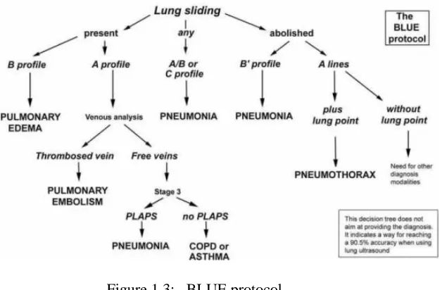
Figure 1.3: BLUE protocol ... 8

Figure 1.4: CT Scans displaying structural changes for pulmonary edema. ... 12

Figure 1.5: CT Scans highlighting structural changes for pulmonary fibrosis... 13

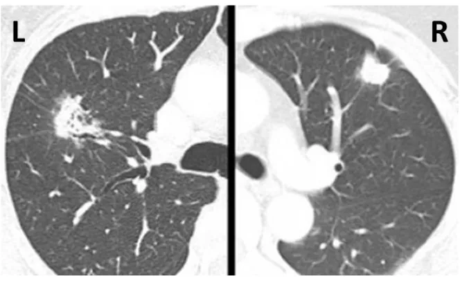
Figure 1.6: CT-Scan of SPN in the lungs. The right lung has a peripheral lesion, which is easier to detect compared to the lesion in the left lung, which is deeper in the lung parenchyma and difficult to detect using palpation ... 14

Figure 1.7: Schematic of VATS ... 15

Figure 2.1: Experimental/Simulation setup showcasing an N element array placed in the near-field of the multiple scattering medium. ... 23

Figure 2.2: Total Intensity, Coherent and Incoherent Intensities obtained from backscattered intensity measurements at any time window T ... 24

Figure 2.3: Growing diffusive halo trend depicted by growing width of the backscattered incoherent intensity ... 25

Figure 2.4: Polar representation of the scattering cross section of a single circular air scatterer at 8MHz scattered in ϴ direction with ϴ=0 representing forward scattering (Also represented by the arrow). ... 27

Figure 2.5: Microscopic image of melamine sponge in its dry state depicting complex network (Scale reads 500 μm) ... 29

Figure 2.6: Geometries with varying volume fractions obtained from image processing of the histology images obtained from a rabbit lung ... 30

Figure 2.7: Experimental Setup for ex-vivo Ultrasound in the Rat lung depicting the eco-graphic gel and the 5ml syringe used to control the air volume fraction in the rat lung ... 32

Figure 2.8: Temporal Evolution of the variance W2 of the Gaussian fit on Iinc. The linear curve of the variance plot provides an accurate measurement of the diffusion constant... 33

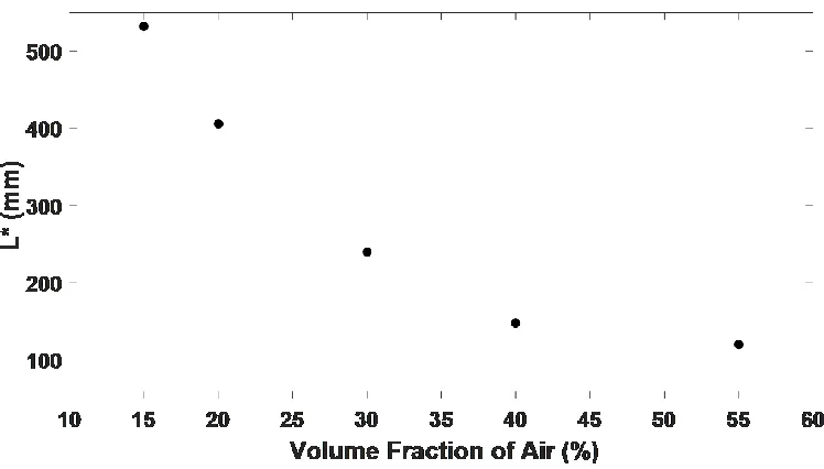
Figure 2.9: L* calculated from simulations for varying volume fractions. ... 33

Figure 2.10: A: Normalized Incoherent intensity as a function of emitter-receiver distance X and time. B: Temporal variance evolution for 20 % and 50 % air volume fraction depicting a rapid growth of the diffusive halo for lower volume fractions... 34

(14)

Figure 2.12: Backscattered received signal with central element (element 64) emitting. ... 36

Figure 2.13: L* in the ex vivo lung as a function of the volume of air removed from the specimen. ... 36

Figure 2.14: L* in the ex vivo rat lung as a function of volume of PBS added to the specimen in use. ... 37

Figure 2.15: Temporal variance evolution for Pig lung depicting growth of diffusion halo over a large range of time. ... 40

Figure 3.1: Schematics of the Geometry used for Simulations and 3D Printed part used for experiments. ... 45

Figure 3.2: Diffusion Constant values calculated from simulations ... 49

Figure 3.3: Experimental and simulation comparison for ABS plastic scattering rods ... 50

Figure 3.4: Simulation and Diffusion Constant (D) map for detection of absence of heterogeneity ... 51

Figure 3.5: Application to SPN size estimation in Pig Lungs ... 52

Figure 3.6: Circular Transducer Set 1 ... 53

Figure 3.7: Circular Transducer Set 1 ... 54

Figure 3.8: Schematic of simulation domain for perpendicular compounding ... 55

Figure 3.9: 1-D diffusion maps in perpendicular direction ... 55

Figure 3.10: 2-D map of lesion obtained from perpendicular compounding ... 56

Figure 4.1: Schematic diagram of splitting the IRM (H(t)) in to sub-IRMs (Hz(t)) ... 63

Figure 4.2: Binarized simulation structure. ... 67

Figure 4.3: Plot of Global diffusion constant (D) vs AF for all simulations ... 71

Figure 4.4: Surface plots for the variance field and linear fit field for the 8mm lesion size, 20mm depth, 20% AF ... 71

Figure 4.5: 2D intensity map the normalized delta field after applying the depression detection filter for the 8mm lesion size, 20mm depth, 20% scatterer fraction. ... 72

iFigure 4.6: A: Final lesion location intensity map. B: Simulation structure. C: Comparison of lesion image with actual structure. ... 73

Figure 4.7: A: Final lesion location intensity map. B: Simulation structure. C: Comparison of lesion image with actual structure. ... 73

Figure 4.8: Lesion detection for 10mm by 5mm elliptical Lesion, 15mm Depth and 20% AF. A: Final lesion location intensity map. B: Simulation structure. C: Comparison of lesion image with actual structure. ... 74

(15)

Figure 4.10: Lesion detection for 10mm Lesion obtained from experimental results, A: Final lesion location intensity map. B: Cross sectional view of the sponge

implanted with petroleum jelly. ... 76

Figure 4.11: Time-Distance approach to calculate effective speed of sound for Air and aluminum scatter ... 78

Figure 4.12: Schematic of memory effect ... 79

Figure 4.13: FDTD Simulation Geometries with varying porosities along the depth... 80

Figure 4.14: Variance plots for memory effect validation ... 81

Figure 4.15: FDTD Simulation Geometries with constant porosities along the depth: ... 82

Figure 4.16: Dependence of D on Porosity ... 83

Figure 5.1: Reflections of the ultrasound beam by thickened interlobular septa give rise to ULCs127. ... 92

Figure 5.2: Non-contrast CT scan images of a normal rat (left), and a rat with pulmonary fibrosis 3 weeks after installation of bleomycin as described (right). ... 94

Figure 5.3: Definition of fibrosis applying with modified scale ... 98

Figure 5.4: Variance growth for in-vivo rodent data Control and Fibrosis ... 99

Figure 5.5: L* Values for in-vivo rat... 100

Figure 5.6: CT Images and their scores ... 101

Figure 5.7: Histology images and their scores ... 101

Figure 5.8: Severity scores based on bleomycin administration time (CT) ... 102

Figure 5.9: Severity scores based on bleomycin administration time (Histology)... 102

Figure 5.10: Comparison between CT and Histology severity scores ... 103

Figure 5.11: Comparison between L* values and Histology severity scores of all 24 rats ... 103

Figure 6.1: CT Scan of Edema with diffused ground glass areas and gravity dependence135_{... 107}

Figure 6.2: B-Lines-a sign of extravascular lung water (Courtesy Lichtenstein140) ... 109

Figure 6.3: Schematic for calculating backscattered frequency shift ... 114

Figure 6.4: ROI definition for evaluating edema ... 116

Figure 6.5: Variance growth for in-vivo rodent data Control and Edema... 116

Figure 6.6: L* values for in-vivo rodent data (Control, Fibrosis and Edema) ... 117

Figure 6.7: Wet to dry ratio for control and edematous lungs and comparison with L* ... 118

Figure 6.8: Spectral functions measuring the frequency decay over depth for edema and fibrosis... 119

Figure 6.9: BFS value comparison for control, edema and fibrosis ... 120

(16)

Figure 6.11: Incoherent intensity and variance growth in regions with and without

B-Lines. A: With B-Lines, B: Without B-Lines ... 122

Figure 6.12: Variance plots for porcine model (Control and Edema) ... 124

Figure 6.13: L* values for control and edema for porcine model ... 124

Figure 6.14: 1-D map of L* in edematous porcine lung without B-Lines ... 125

Figure 6.15: 1-D map of L* in edematous porcine lung with B-Lines ... 126

Figure 6.16: Incoherent intensity and variance growth in regions with and without B-Lines.A1: Without B-Lines,A2: With B-Lines, B-Diffusive halo growth ... 127

Figure 6.17: L* values for ex-vivo porcine lung at different tidal volumes... 129

Figure 7.1: 3MHz Signal in time and frequency domain ... 136

Figure 7.2: Mono-disperse bone schematic geometry, A: ϕ =50 μm, ρ = 3 pores/mm2, B: ϕ =120 μm, ρ =16 pores/mm2 ... 138

Figure 7.3: Poly-disperse bone schematic geometry, A: ϕ =50 μm, ρ = 16.85 pores/mm2, ν=0.047, SD=33 μm, B: ϕ =71 μm, ρ =14.3 pores/mm2, ν=0.081, SD = 47 μm ... 139

Figure 7.4: Frequency dependent attenuation for mono-disperse FDTD simulation ... 140

Figure 7.5: Frequency dependent attenuation for poly-disperse FDTD simulation ... 141

Figure 7.6: Schematic of the ANN structure. The arrows depict connection between neurons of 2 layers ... 142

Figure 7.7: Attenuation trends at Frequency =8MHz, A: Fixed pore diameter, B: Fixed pore density ... 143

Figure 7.8: ANN Results for Mono-Disperse data only ... 145

Figure 7.9: Attenuation plots for varying pore diameters and pore sizes. ... 146

Figure 7.10: ANN Results for Poly-Disperse data only ... 147

Figure 7.11: ANN Results for Mono and Poly-disperse combined data (Unified Model) ... 148

Figure A.1: Experimental/Simulation setup showcasing an N element array placed in the near-field of the multiple scattering medium. ... 184

Figure A.2: Real part of matrix K obtained in a sponge at time T = 27 µs and 4.9 MHz ... 185

Figure A.3: Principle of the separation between the single and multiple scattering contributions ... 187

Figure A.4: Ratio of MS and SS over time ... 188

Figure A.5: Backscattered Intensities for the sponge case. ... 189

Figure B.1: Schematic diagram of splitting the IRM (H(t)) in to sub-IRMs (Hz(t)) ... 196

Figure B.2: Lesion at 15mm Depth, 10Vf... 199

(17)

(18)

CHAPTER 1 - Introduction

1.1 Challenges in Imaging Heterogeneous Biological Tissues

Sonography is a very effective technique, which uses ultrasound waves to create an image of the body for diagnosis purposes. The concept of ultrasound imaging is based on echolocation. The working principle of ultrasound imaging uses a transducer emitting a pulse of high frequency mechanical wave, which propagates through the tissue. It undergoes multiple phenomena as it propagates which can be divided into reflection, transmission and scattering. These phenomena can be seen when the wave moves from one medium into another. The beam is partly reflected back at the tissue interfaces. Backscattered signals when plotted using a Hilbert transform generates an ultrasound image. In most human tissues, ultrasound imaging is possible due to similar acoustic impedances. However, for media such as the bone (bone water matrix) or lungs (tissue air matrix) the attenuation is very high and the received signal (Figure 1.1) is very complicated making it hard to reconstruct the micro-architecture of the lung.

(19)

Lung ultrasound characterization has remained elusive due to the presence of air-filled alveoli and the very complex micro-architecture of the lung tissue. The lungs at the peripheral regions can be considered a porous media with alveolar air sacs, which act as scatterers when the ultrasound wave propagate through it (Figure 1.2). As the wave interacts with the alveolar sacs large specular reflections are also noticed due to the drastic impedance change between tissue (ρ=990 kg/m3_{, c = 1540 m/s) and air (ρ=1.00 kg/m}3_{, c = 340 m/s). These specific properties of the} lung tissue are responsible for ultrasound multiple scattering, a regime in which the waves do not propagate straight, and in which the linear relationship between propagation time and propagation distance is lost1–4, which alters conventional ultrasound imaging. There is large absorption and dispersion features which are yet to be quantified and only preliminary work has been done ex-vivo4. In this thesis, we propose an innovative method in which we exploit ultrasound multiple scattering by the alveoli to quantitatively characterize the lung parenchyma. Indeed, each scattering event can be seen as an opportunity for the wave to embed information on the micro-architecture of the parenchyma.

(20)

Multiple scattering and wave propagation in disordered media is a very complicated subject which has undergone tremendous change in the last 40 years. Anderson’s introductory work on wave localization phenomena was a landmark in this research5–7. For very complex waves in disordered media, a coherent understanding has only very recently emerged. Since a localized wave does not have spatial periodicity, there was a requirement for a completely new theoretical framework. A consolidated approach was presented in the book written by P.Sheng 8_which consolidated all theories explaining mesoscopic phenomena which are the ideal manifestations of wave scattering and interference effects. For infinite media, the wave propagates in a known direction with a known velocity. However, when scattering is involved, the original direction of propagation is lost and more often than not, the wave enters an Omni-directional or a radially growing wave diffusive regime9–12. This diffusion of the wave in a scattering medium is characterized by the diffusion constant D. This D is found to have strong dependence on the wavelength λ as well as the scatterer size d in the inhomogeneous media, which is being insonicated with ultrasound. There are two major considerations for quantifying wave diffusivity and analyzing the wave diffusion regime. One is the scatterer size d and its packing fraction. The second consideration is the wavelength λ. The ratio d/λ helps in determining the average distance

of coherent propagation between two scattering events. This distance is referred to as the mean free path and d/λ is the relevant length scale in demarcating the different wave regimes. For d/λ

<<<<1 the scattering is very weak. For a scale of a few mean free paths, the medium can be considered as an effective homogeneous medium. However, over multiple length scales(multiple mean free paths), this assumption does not hold true. Once the multiple scattering starts dominating, the wave enters a diffusive transport regime. For d/λ>1, the diffusive transport regime

(21)

using the coherent and the incoherent waves. It is becoming a widely studied phenomenon and both the backscattered coherent and the incoherent waves have been proved useful to characterize disordered media, exploiting coherent and incoherent effects in classical, electromagnetic or acoustic waves 13–21.

1.2 Current State of the Art in Lung Ultrasound

(22)

sensitivity. X-Ray beam origination is not tangential to the diaphragmatic cupola thereby hindering correct interpretation of the thoracic structures 23,30.

(23)

MRI is also associated with high acquisition times, poor spatial resolution and non-qualitative approach makes it a challenge in diagnosis of pathology.

(24)

high when acquiring data for human lung parenchyma. CT when combined with other imaging modalities increases its specificity and sensitivity. A multitude of work has been done combining CT with PET, MR and optical flow imaging which has shown promise in diagnosis and response to treatment of pathologies26,27,36.

(25)

Figure 1.3: BLUE protocol

(26)

using diffused bilateral B-Lines can be used to characterize community acquired pneumonia (CAP) and AIS. Indeed, Lung US is an easy-to-use, low-cost technology that allows accurate non-invasive bedside assessment of pulmonary pathologies. Its usefulness is related to the easy detection of certain specific vertical artefacts called B-lines. Lung US saves time and cost, provides immediate information to the clinician and relies on very easy-to acquire and highly reproducible data.

The fundamental issue with all these works are that the interpretation of these B-Lines is highly operator dependent and qualitative in nature. We now shift our focus to highlight the quantitative work done in LUS.

1.3 Quantitative Ultrasound and Diffusion Measurements

(27)

quantification of lung tissue since the single scattering approximation does not hold true. A potential methodology for characterizing is measuring the speed of the surface wave using an external agitator to generate surface waves at different frequencies. Zhang et al57,58 showed that for fibrotic lungs, the surface waves propagated at much higher velocities than for control cases. This was due to the presence of stiffer tissue. In 2016, Zenteno 59et al. were able to detect pneumonia even at early stages using a spectral based methodology where the frequency based attenuation was used to characterize the lung parenchyma. Although in its very nascent stages, Demi et al 60_{recently proposed a potential quantitative method to characterize the lung using} spectroscopy. They noticed that the B-Lines do not always appear for a given lung and only appear at certain frequencies. Hence it could be concluded that the B-Lines themselves are frequency dependent and this is something that should be looked into in the near future.

(28)

approach developed by Aubry et al. was successfully tested on a phantom consisting of steel rods in water 16. D is a single number characterizing a scattering medium. In a multiple scattering medium, when the wave enters the diffusive regime, D is used to characterize the rate at which the diffusive halo grows. Derode, Aubry and Shahjahan64–68 then developed a methodology using singular value decomposition (SVD) to separate multiple scattering and single scattering contributions in a heterogeneous media. This allowed them to isolate the single scattering contribution, which in general is used for generating B-Mode images in sonography. Using a multiple scattering filter, they were able to identify targets/lesions, which allows visualization of defects in a system. Multiple scattering has also been used to characterize complex soft tissues. In this thesis, we demonstrated that the diffusion constant D is relevant to the assessment of alveolar interstitial syndrome and more specifically pulmonary edema and pulmonary fibrosis.

1.4 Pulmonary Fibrosis and Edema

(29)

Figure 1.4: CT Scans displaying structural changes for pulmonary edema.

Pulmonary fibrosis is a progressive, fatal, inflammatory and fibro-proliferative lung disease for which existing treatments are of limited benefit74–76. Past data have suggested that it is the most common chronic interstitial disease.

We try to look at detection of fibrosis and edema in a very simplified manner. Both pulmonary edema and fibrosis lead to structural changes in the micro-architecture of the lung parenchyma. In fibrosis, the thickening of the alveolar walls (Figure 1.5) reduces the compliance and the volumetric intake of air due to the reduction in the effective size of the air sacs77. In the case of edema, the alveolar sacs are filled with water, which also reduces the effective volume of the lung and its elasticity. Due to these structural changes, we hypothesize that in case of AIS, the effective amount of multiple scattering is much lower which allows the wave to diffuse deeper compared to a healthy lung. In a healthy, normal lung, the millions of air-filled alveoli are responsible for frequent scattering events, leading to short mean free paths.

(30)

Figure 1.5: CT Scans highlighting structural changes for pulmonary fibrosis.

In this thesis, we demonstrate, for the first time, that ultrasound multiple scattering, usually considered an obstacle to imaging highly scattering media, can be taken advantage of, in characterizing AIS in the lung parenchyma. We propose to analyze the backscattered signals to obtain the diffusivity of the lung parenchyma to characterize the lung using wave transport parameters, namely the diffusion constant D and the mean free path 13.

1.5 Lesion Detection

(31)

For early lung cancer, VATS has been adopted as an important tool in the treatment of this disease through minimally invasive surgery. Low dose CT has been shown to be effective in the early detection of lung cancer, thus reducing mortality rates83–85. However, the nodules requiring resection detected by screening are smaller. The difficulty of palpating makes VATS resection of deep-seated nodules or ground glass opacities hard. Successful VATS for the resection of pulmonary nodules depends on intraoperative nodule identification by direct visualization or palpation in the past. With the increased use of low dose CT, greater numbers of small lung lesions are detected. Not only size but also distance to the pleural surface can influence the nodule detection rate using palpation during VATS. Deep-seated solitary pulmonary nodules are difficult to palpate during VATS

Figure 1.6: CT-Scan of SPN in the lungs. The right lung has a peripheral lesion, which is easier to detect compared to the lesion in the left lung, which is deeper in the lung parenchyma and difficult to detect

using palpation

(32)

good-quality ultrasound images in 56% of patients89_{. However these high number were attributed} to two reasons. Firstly, these lesions were at the periphery or adjacent to the pleural line. Secondly deeper GGOs were identified using ultrasound using completely collapsed lungs. GGO is similar to adjacent normal lung tissue in density and thus localizing them with ultrasonography is hard, even for experienced chest surgeons. In a healthy, partially inflated lung, ultrasonography has been deemed unusable. Some pilot studies have measured the chance of detecting tiny pulmonary lesions including GGO with ultrasonography to define the limitation as well as help surgeons improve their skills90_{. Based on the study done by Dunn and Fry}3,4,91_{the attenuation is very high} in the lung parenchyma, even when the lung is collapsed under atmospheric pressure. Many of the clinical reports on intraoperative thoracic ultrasonography emphasize the need for thorough deflation of the lungs or atmospheric collapse of the lungs82,92–97.

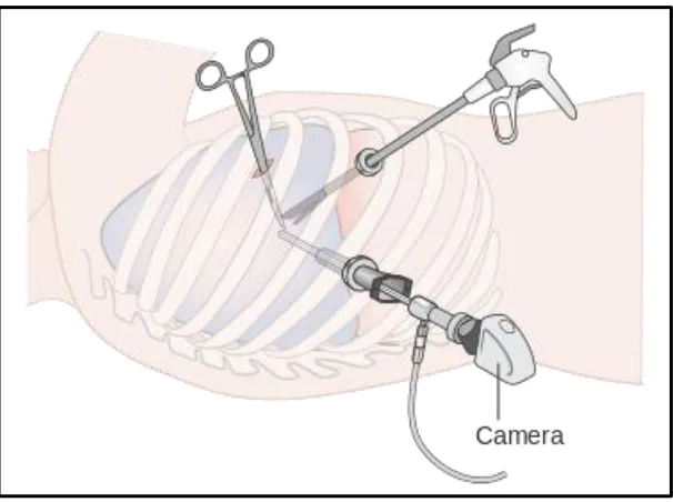
Figure 1.7: Schematic of VATS

(33)

to locate by surgeons viewing the partially collapsed lung during VATS. Surgeons may insert their finger in the thoracic cavity via another incision, bring the lung tissue to their finger and try to palpate the nodule. However, SPN can be extremely difficult to locate precisely. Small nodules might be extremely difficult to feel82,89. Therefore, there is no guarantee that the nodule will be in the resected region of the lung parenchyma, or that the margins will be adequate. Conventional ultrasound to visualize SPNs has been described, but the lung must be completely atelectatic to visualize nodules82. None of these methods enhances the likelihood of a clear resection margin. VATS wedge resection is being used increasingly as definitive therapy. A positive margin leaves tumor behind and substantially reduces the chance of cure.

(34)

1.6 Roadmap of Chapters

From Chapter 2 to Chapter 4, the thesis explains in details the development of the diffusion algorithm. Each chapter between 2 to 4 addresses the analytical model, data acquisition, algorithm development and its validation both computational and experimental. Chapters 5-7 then delves into the clinical application of the algorithms discussed in the previous chapters. Each chapter describes the data acquisition and challenges, and how the data was processed before the diffusion algorithms were applied on them. The diffusion constant D measures the effective properties of the media which are non-local in essence. However, we explain how we have this methodology extended to 1D imaging and further into 2D imaging to generate 2D diffusion maps. Chapter 2 will discuss how the basic Diffusion measurement algorithm was developed. Chapters 3 and 4 will describe a new diffusion mapping methodology. Chapters 5 and 6 will discuss the applications of using D to characterize the healthy lung parenchyma in rats and differentiating it from pulmonary edema and pulmonary fibrosis. Chapters 5 and 6 will also encase preliminary clinical data obtained from larger animals. Chapter 6 will then discuss an algorithm, which is developed to ensure the unequivocal diagnosis of edema and fibrosis.

(35)

CHAPTER 2 – Diffusion Theory and Transport Parameters

2.1 Abstract

(36)

2.2 Introduction

The ultrasonic quantitative characterization of the lung parenchyma has remained elusive due to the presence of air-filled alveoli and the very complex micro-architecture of the lung tissue. These specific properties of the lung tissue are responsible for ultrasound multiple scattering, a regime in which the waves do not propagate straight, and in which the linear relationship between propagation time and propagation distance is lost, altering conventional ultrasound imaging. In the present paper, we propose a method in which we exploit ultrasound multiple scattering by the alveoli to quantitatively characterize the lung parenchyma. Indeed, each scattering event can be seen as an opportunity for the wave to embed information on the micro-architecture of the parenchyma. Multiple scattering is becoming a widely studied phenomenon and has been proved useful to characterize disordered media, exploiting coherent and incoherent effects in classical, electromagnetic or acoustic waves 13,14.

Conventional lung imaging is generally done using chest radiography (CXR) or thoracic computed tomography (CT) 22. Both these imaging modalities have limitations, which puts a constraint to their applicability. CXR is constrained by limited diagnostic performance, portability of bedside radiography and X-Ray exposure issues. Due to the moving thorax, the spatial resolution decreases and leads to poor-quality X-Ray films with low sensitivity. X-Ray beam origination is not tangential to the diaphragmatic cupola thereby hindering correct interpretation of the thoracic structures 23,30. Although thoracic CT is the gold standard for lung imaging, it is very costly, and transportation of the critically ill to the concerned department combined with radiation exposure increases the measurable risk.

(37)

effusion, and consolidation 45,46_{. Lung ultrasound has also garnered a large applicability in} detection of pulmonary manifestations of neonatal respiratory distress syndrome 47. Lung ultrasound is arguably the fastest and most effective method to detect diaphragmatic paralysis and diagnosing pleural effusion, especially when trying to differentiate between effusion and consolidation 48. Due to its portability and removed irradiation effects, lung ultrasound has become an option for thoracic imaging in the critically ill. The conventional approach of lung ultrasound is based on the identification of ten standardized signs: the bat sign (pleural line), lung sliding (yielding seashore sign), the A-line (horizontal artefact), the quad sign, and sinusoid sign indicating pleural effusion, the fractal, and tissue-like sign indicating lung consolidation, the B-line, and lung rockets indicating interstitial syndrome, abolished lung sliding with the stratosphere sign suggesting pneumothorax, and the lung point indicating pneumothorax 45. However, reading and interpreting these signs is subjective and operator-dependent. Lung ultrasound imaging past the pleural layer is highly inaccurate because of the presence of multiple scattering in the parenchyma occurring from drastic changes in impedance from tissue to air in the alveoli. During lung imaging, the backscattered signals are distorted, leading to artefacts and introducing large errors in reading and interpreting the images 49.

(38)

human trabecular bone which is highly complex and diffusive in nature 63_{. The approach developed} by Aubry et al. was successfully tested on a phantom consisting of steel rods distributed in water 16_{. The diffusion constant, as demonstrated in this paper is relevant to the assessment of lung} edema, and air volume fraction in the lung. We demonstrate, for the first time, that ultrasound multiple scattering, usually considered an obstacle to imaging highly scattering media, can be taken advantage of in characterizing the lung parenchyma.

Due to the very strong impedance difference between the lung tissue and the alveoli, it is assumed that the tissue acts as the propagating medium whereas the alveoli play the role of scatterers. As reported in earlier studies, the lung parenchyma can be treated as a sponge whose volume fraction varies during inhaling and exhaling. Numerous studies have been performed using ultrasound as well as magnetic resonance imaging using gelatin sponges as a lung-mimicking phantom 98,99. Spinelli et al. used a gelatin sponge to act as a simplified structure of the lung in order to reproduce its viscoelastic properties and generate a simplified model, which can be used to reproduce mechanical, architectural and acoustic properties of pulmonary tissues. Earlier models developed from culturing of pulmonary epithelial cells were complex and identified as a major challenge 98.

(39)

2.3 Diffusion Principe

2.3.1 The Incoherent wave

The objective was to measure the diffusion constant D and the transport mean free path L* of the entire geometry based on the dynamic backscattered incoherent intensity. The method for processing the inter-elements response matrix, or impulse response matrix (IRM) was developed upon the work previously done by Aubry et al. The IRM (H(t)) has a unique feature of reciprocity (hij(t) =hji(t)) 13,16. Using this observation, another matrix, called HA (t) was defined as follows: 16

for i>j, hijA=-hij; for i= j, hii=0; for i<j, hijA_=hij;

It is to be noted that HA(t) is a fictitious matrix. The temporal variation of the incoherent intensity exhibits the unique property of a growing diffusive halo, which can be visualized. The intensities were calculated for H(t) by appropriately time shifting the backscattered signals so as to ensure that the received signals arrive at the same time on every transducer. The time signals hij(t) were then truncated in 0.3µs overlapping windows:

ij ij R

(40)

Figure 2.1: Experimental/Simulation setup showcasing an N element array placed in the near-field of the multiple scattering medium.

A short time FFT provided a response matrix called K(T,f) for each time window T. Each element of K(T,f) is represented as kX

EXR(T,f) corresponding to the responses at the frequency f and time T between the emitter location (XE) and the receiver location (XR) as shown in Figure 2.1.The backscattered intensity (I(X, T)) was calculated by integrating the squared values of the kX

EXR(T,f) for all emitter/receiver couples (denoted by < |kXEXR(T,f)|

2_{> in Equation 2) by that are}

separated by the same distance X = |XE-XR| 16.

E R E R

2

X X f,{X ,X }

I(X,T)=<|k (T,f)| > (2)

The HA (t) matrix was processed in a similar fashion to obtain the IA(X,T). The backscattered intensity can also be obtained in the time domain by squaring and integrating kX

EXR(T,t) over time and over emitter/receiver couples separated by the same distance X = |XE - XR|.

E R E R

2

X X t,{X ,X }

I(X,T)=<|k (T,t)| > (3)

(41)

𝐼_𝑖𝑗(𝑇) = ∫_𝑇−𝑇+𝑡/2𝑡 ℎ_𝑖𝑗2(𝑡)𝑑𝑡 2

(4)

Where 𝑇 is the time at the center of the time window and t is the width of the time window.The backscattered intensity 𝐼(𝑋,𝑇) was calculated by averaging 𝐼𝑖𝑗(𝑇) over the emitter-receiver pairs

separated by the same distance 𝑋=|𝑋E−𝑋R| .

2.3.2 Measuring the Diffusion constant using the Growth of the Diffusive Halo

Normalized intensities IA and I, obtained from HA(t) and H(t) respectively, were used to evaluate the incoherent intensity using I_inc =I+IA

2 .

Shown in Figure 2.2 is an example of the total backscattered intensity and its split up into its coherent and incoherent component. We seen that the coherent component is only seen when the distance between the emitter and receiver is 0, that is the emitter and receiver are the same.

(42)

In highly scattering media, the propagation of the incoherent intensity obeys the diffusion equation and, in the near-field approximation, the incoherent intensity can be expressed as a function of the diffusion constant D:

2 inc

X I (X,T)=I(T)exp(- )

4DT (5)

Where X represents the distance between emitter and receiver. Equation 5 clearly illustrates that the incoherent intensity over time describes the growth of the diffusive halo 16. The incoherent intensity Iinc was plotted as a function of time and emitter-receiver distance (X=|XE-XR|). All intensities corresponding to the same emitter-receiver distance X were averaged. For each time window, the spatial spread of Iinc was fitted with a Gaussian plot and the variance of the Gaussian plot was calculated. The variance (W2_{(T) = 2DT) of Iinc represents the dynamic growth of the}

diffusive halo. When W2(t) is plotted against time, half of the slope of the linear fit is the diffusion constant D. The growing trend of the backscattered incoherent intensity is shown in Figure 2.3.

(43)

2.3.3 Mean free paths

The transport mean free path L* is associated with the diffusion constant D through the equation 100,101

E

V ×L* D=

3 (6)

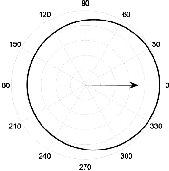
Where VE is defined as the transport speed, and is taken to be the speed of sound in tissue (1.575 mm/µs). In the present study, the scatterers are the air-filled alveoli, which have been approximated as spherical air pockets in the tissue. In order to determine the relationship between the various mean free paths (transport, elastic, and scattering mean free paths), a simulation of ultrasound scattering by a circular air sac in 2-D were carried out using SimSonic, an open source simulation software based on Finite Differences Time Domain 102,103. Analysis of the pressure field by a single circular air sac was performed to estimate the average cosine of the scattering angle cosϴ by one such scatterer 13,103,104_{. A plane wave of central frequency 8MHz was emitted} into the medium with a single circular air scatterer of 100μm diameter. The scattered signal was recorded by placing a circular array of receivers surrounding the single alveola at a distance of 300 μm from its edges. The simulation was repeated without the scatterer. The two signals recorded on the receivers were subtracted so as to obtain only the scattered signal, providing the normalized scattered intensity as a function of the scattering angle. The average cosine of the scattering angle is calculated using the formula.

2Π 0

1 dσ(θ)

cosθ= cos(θ) dθ

2



dθ (7)

Where dσ(ϴ)

dϴ is the differential scattering cross section and σ is the total scattering cross

(44)

direction obtained as described above. This shows that air-filled alveoli are quite an isotropic scatterer.

Figure 2.4: Polar representation of the scattering cross section of a single circular air scatterer at 8MHz scattered in ϴ direction with ϴ=0 representing forward scattering (Also represented by the arrow).

The average cosine of the scattering angle cosϴ was found to be 0.0514. The isotropic scattering nature of such a circular scatterer can also be extended to 3-D. A challenge in the lung parenchyma is the existence of alveoli with varying diameters, however since the scatterers are fairly spherical air sacs, cosϴ will be very small for any scatterer diameter. The simulation for the air sac scatterer was performed to obtain a relationship between the elastic mean free path (Ls) and the transport mean free path (L*). Ls and L* are related to each other by the equation 13

s

L L*=

1-cosθ (8)

(45)

2.4 Validation Methodology

2.4.1 Ultrasound Experimental setup

In both simulations and experiments, ultrasound pulses were transmitted using single elements of a linear transducer array, one by one. For all numerical simulations, a 64 elements linear array with a central frequency of 8 MHz was simulated. For all experiments, a 128 element Verasonics L11-4v linear array was used, connected to a Verasonics Vantage ultrasound scanner (Verasonics, Kirkland, WA). The transducer was coupled to the lung by a layer of ultrasound coupling gel (approximately 5 mm). In both simulations and experiments, all of the elements of the array were fired one by one, transmitting a 2 cycles pulse with a central frequency of 8 MHz into the medium. For each transmitted pulse, the backscattered signals were collected on all elements of the array, which gave access to the spatial spread of the transient pressure field. This enabled the acquisition of the 128 by 128 (64 by 64 for simulations) inter-element response matrix H(t) whose individual elements are hij(t) where i is the emitter number and j is the receiver number. The individual elements hij(t) are the N2 inter-element responses of the probe-medium system. 13,16,105_.

2.4.2 Sponge Phantom Experiments

(46)

carried out within 30 seconds of obtaining the desired volume fraction. Figure 2.5 is a microscopic image (NIKON eclipse LV150 optical microscope) of the melamine sponge used in its dry state. It depicts the complex network of the melamine in which water saturation reduces the number of air-filled pores. This network was assumed to mimic the lung parenchyma’s multiple scattering properties.

Figure 2.5: Microscopic image of melamine sponge in its dry state depicting complex network (Scale reads 500 μm)

2.4.3 FDTD Simulations

(47)

wavelength). A 64 element linear transducer with a central frequency of 8 MHz and element width of 0.3 mm was simulated.

Figure 2.6: Geometries with varying volume fractions obtained from image processing of the histology images obtained from a rabbit lung

2.4.4 Animal experiments

(48)

evaluation was carried out using an L11-4v linear array transducer with central frequency of 8MHz connected to a Verasonics Vantage ultrasound scanner. The IRM was acquired as described above. Heparin (600 U; Elkins-Sinn, Cherry Hill, NJ) was injected intra-hepatically. Five minutes later, the pulmonary artery was cannulated through the right ventricular outflow tract with a length of p60 tubing. The right and left atrium were incised, the endotracheal tube was clamped at end of inspiration, and the lungs were flushed with 20 ml cold (4°C) Perfadex buffered with THAM (XVIVO Perfusion Inc., Denver CO) from a height of 20 cm. The heart lung block was then excised. This removes all blood from the lungs, and is analogous to how human lungs are recovered for transplant. The blood was drained out in order to avoid clotting and to ensure that only the alveoli sacs participate in the scattering phenomena. Ideally, this would result in the absence of erythrocytes in the capillaries, however perfadex was present which would not hamper the ultrasound wave propagation due to similarities in the acoustical properties of blood and perfadex. After surgical ligation of the lungs, a polyethylene tube was inserted into the trachea, which was connected to a three way stop-cock of which one end was connected to a 5ml capacity syringe. This allowed control over the air volume fraction and avoided air leakage. Once the lungs were excised, the ex vivo ultrasound evaluation was performed by applying coupling gel directly on the surface of the lung. All ex vivo experiments were conducted within 12 hours of death of the rat.

(49)

Figure 2.7: Experimental Setup for ex-vivo Ultrasound in the Rat lung depicting the eco-graphic gel and the 5ml syringe used to control the air volume fraction in the rat lung

Animal Studies: This study was approved by the Institutional Animal Care and Use Commit-tee of the University of North Carolina at Chapel Hill. All animals received humane care in

accordance with the Guide for the Care and Use of Laboratory Animals (National Academy Press, 1996).

2.5 Results

2.5.1 Numerical Simulations

(50)

Figure 2.8: Temporal Evolution of the variance W2 of the Gaussian fit on Iinc. The linear curve of the variance plot provides an accurate measurement of the diffusion constant.

L* as a transport parameter was highly correlated to the air volume fraction (r=-0.9542, p<0.0117). Figure 2.9 shows the variation of L* as a function of increasing volume fraction ex vivo.

(51)

2.5.2 Phantom experiments: Sponge study

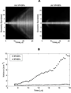
The experiments, carried out on the 50 cm3 blocks of sponge, were repeated five times so as to test the repeatability of the measurement on a given geometry. For each air volume fraction, the growth of the diffusive halo was estimated over time, enabling the measurement of L*. When the incoherent intensities were plotted against time, the growth of the diffusive halo could be tracked as shown in Figure 2.10A.

Figure 2.10 A: Normalized Incoherent intensity as a function of emitter-receiver distance X and time. B: Temporal variance evolution for 20 % and 50 % air volume fraction depicting a rapid growth of the

(52)

Figure 2.10B shows a comparison between the temporal evolution of the variance for 20% and 50% volume fraction. It is very clear from the variance plots that the growth of the diffusive halo is very restricted for higher volume fractions of air whereas it is much more rapid in lower volume fractions of air. With increasing air volume fractions, the amount of water decreased thereby reducing D and the derived L* values.

Figure 2.11 shows L* as a function of air volume fraction in the sponges. The error-bars are the standard deviation obtained from five consecutive readings obtained for each air volume fraction. A strong correlation (r=-0.9932, p<0.0068) was also observed between L* and the air volume fraction.

Figure 2.11: L* calculations for varying volume fractions in sponge phantom

2.5.3 Ex vivo Rat Lung with Varying Air Fraction

(53)

measurement was repeated 4 times in order to estimate the repeatability of the method. Figure 2.12 shows the backscattered signals on the 64th element of the linear probe as an example.

Figure 2.12: Backscattered received signal with central element (element 64) emitting.

L* measured in the ex vivo rat lung as a function of air volume fraction are shown in Figure 2.13. The errorbars shown on Figure 2.13 are the standard deviation of a distribution of 4 consecutive measurements, and demonstrate the repeatability of the measurement.

(54)

2.5.4 Ex vivo Rat Lung with PBS Addition to Simulate Edema

Instead of air, 1ml, 2 ml, and 3 ml of phosphate-buffered saline (PBS) was progressively added to the lung ex vivo via a syringe. PBS proved to be a better solution to engineer edema in the lungs because of its non-toxicity to most cells and isotonic nature. For each PBS volume fraction, the IRM was acquired and the L* values were calculated as described above. Figure 2.14

shows a plot of L* as a function of amount of PBS added to the rat lung.

Figure 2.14: L* in the ex vivo rat lung as a function of volume of PBS added to the specimen in use.

2.6 Discussion

(55)

single scatterer simulations using FDTD showed that the approximation that transport mean free path, scattering mean free path and elastic mean free path are similar is reasonable, as suggested by the calculation of the average value of the cosine of the scattering angle of a single scatterer, described above 100,101.

The approach developed for analyzing the incoherent intensities showed promising results for the characterization of the lung parenchyma. By varying the amount of fluid, we were able to mimic a variety of air volume fractions. For every change of 10% in the fluid volume fraction, L* was seen to vary by an order of 100 μm. This can be attributed to the fact that when fluid saturation increased, the hollow spaces in the sponge network or in the parenchyma were increasingly occupied by fluid, which increased the distance between two scattering events on average.

The melamine sponge saturated with water doesn’t perfectly replicate tissue properties of the lung parenchyma. However, the basic micro-architecture of the cross linked sponge generates a multiple scattering medium which replicates the strong multiple scattering effects observed in the lung parenchyma due to the presence of air. The purpose of the melamine sponge experiments was to work in media with a controlled amount of saturating fluid. This enabled us to validate our quantitative approach for the calculations of the transport mean free path. The present study demonstrates that changes by 10% of the water volume fraction were easily detected, and lead to variations in the mean free path that were much larger than the error-bars. A thorough sensitivity study remains to be conducted in order to determine the lowest possible change of water volume fraction detectable by the method, and will be the subject of a further study.

(56)

vivo. However, other pathologies such as pulmonary fibrosis are likely to result in similar changes in the air volume fraction, although the water content in the fibrotic lung does not change. Compared to the acoustic impedance of the air-filled alveoli, the acoustic impedance of fibrotic tissue is likely to be similar to that of water. As a consequence, discriminating between pulmonary fibrosis and pulmonary edema using the present method might be challenging. This will be investigated in a further study, where we will compare in vivo models of fibrosis and edema in the rat. The change in L* due to addition of water was more prominent compared to the change in L* due to addition of air. This can be attributed to the near incompressibility of biological tissues.

(57)

lung ex vivo. The pig lung was connected to a ventilator and fully inflated in order to maximize the air volume fraction. Figure 2.15 shows that the growth of the diffusive halo can be tracked over 25s. No specular reflection from the back of the lung could be observed in the backscattered signals. The calculated D value was observed to be 0.17mm2_{/μs and the corresponding L* value} was found to be 323μm.

Figure 2.15: Temporal variance evolution for Pig lung depicting growth of diffusion halo over a large range of time.

2.7 Conclusion

(58)

(59)

CHAPTER 3 - 1-Dimensional quantitative micro-architecture mapping of

multiple scattering media

3.1 Introduction

Multiple scattering, is an obstacle to imaging but carries a lot of potential for the characterization of the microarchitecture of complex heterogeneous media. Multiple backscattering signals carry information about the diffusivity of disordered media, when quantified, enables the characterization of their micro-architecture (density or porosity)8,12,62. A method described by Tourin et al. 13 based on coherent back-scattering106,107 in the far field, measures the diffusion constant D. The information carried by the coherent contribution to scattering is relevant if the scattering is weak (weak localization)13,6,15. Furthermore, the coherent contribution can only be exploited in the far field13,17,105. In highly disordered media, the incoherent contribution to the backscattering embeds information on the micro-architecture that can be exploited as well. This letter focuses on applications where far-field conditions can’t be achieved. Hence, incoherent backscattered contributions, which have been observed in various applications19,21,108 becomes the key parameter to predict the diffusivity of a medium.

(60)

ultrasound (EBUS) to characterize the lung parenchyma for cancer staging109_{using multiple} scattering or detect solitary pulmonary nodules/lymph nodes16. Currently EBUS is used to perform needle biopsies of peribronchial lymph nodes. However, if EBUS was used to characterize the lung parenchyma, near-field assumptions would be necessary. For EBUS lung characterization or peripheral nodule imaging, far-field conditions cannot be achieved and multiple scattering starts occurring approximately at the transducer surface. The assumption behind the present method is that in the near field, the incident and backscattered waves are directive enough and Gaussian Beamforming is not required. If the source and the receivers are directive enough and located in the near-field, the incoherent intensity exhibits the growth of the diffusive halo. Placing the transducer at the surface of the sample corresponds to a near-field configuration with the incoherent backscattering intensity showing a well characterized time dependence21. We demonstrate that such a typical behaviour can also be observed with conventional linear array transducers. We use finite difference time domain (FDTD) simulations of circular plastic scatterers in water and show experimental validation with plastic (Z=2.31MRayl) cylindrical scatterers in water. Since plastic is not a strong scatterer, we also validate this near field approach using aluminium (Z=17.1MRayl) circular scatterers in water using FDTD. All FDTD simulations are carried out in 2-D.

3.2 Materials and Methodology

(61)

4cm x 4cm phantom is divided in 5 sections with VF of scattering rods of respectively 5%, 10%, 15%, 20% and 25%. Due to the lower resolution of the metal printer available, the diameter of the scattering rods (0.5mm) and relatively high VF, the phantom had to be 3D printed using ABS plastic instead of metal, which would have provided stronger scattering.

Finite differences time domain (FDTD) simulations were carried out for two separate media. The geometries consisted of circular Aluminium scatterers (ρ=2.7g/cm3_{, Speed of} Sound=6.32mm/μs, E=70GPa) and ABS circular scatterers (ρ=1.05g/cm3_{, Speed of} Sound=2.25mm/μs, E=1.4GPa), randomly distributed in water (ρ=1g/cm3_{, Speed of} Sound=1.5mm/μs), with controlled VF. The 4cm x 4cm geometry was divided into 5 sections with varying VF 5%, 10%, 15%, 20% and 25%. The purpose of simulations is twofold. Firstly, using plastic scatterers, we validate this methodology and compare with experiments. Secondly, using aluminium scatterers, we also highlight the efficiency of this methodology for strong scatterers. Simulations were performed in 2D using SimSonic102,110_{, an open-source FDTD simulation tool.} The spatial grid step was 0.02mm (approx. 15 points per wavelength). The CFL (Courant-Friedrichs-Lewy) condition was set to 0.999. The time step was defined according to the scatterer.

Experiments were conducted in a water tank. Signals were acquired using a 128 element ultrasonic array (L7-4) connected to a Vantage Verasonics (Verasonics, Kirkland, WA) operating at a central frequency of 5.1MHz. A voltage of 30V was used to improve signal to noise ratio (SNR) since acoustic pressures are low due to single element emission. In the current in vitro and

(62)

of the phantom and the transducer was the same. The transducer lateral axis was placed along the varying VF.

Figure 3.1: Schematics of the Geometry used for Simulations and 3D Printed part used for experiments.

Both the experimental and simulation setups consisted of a 128 element linear array transducer with pitch 0.31mm. Given the dimensions of the transducer elements, and analytical calculations by Marini and Rivenez111, the near field was between 0.35λ and 88λ. In the present case, the transducer was approximately 1mm away from the surface of the medium, with either water or a thin layer of coupling gel in between. This corresponds to approximately three wavelengths in water, which ensures near field conditions. An IRM (inter-element Response Matrix21,108) was acquired by emitting 2-cycle pulses at 5.1MHz with single transducer elements one by one, and by recording the backscattered echoes on all elements for every transmit, for 40μs. The process was repeated until the backscattered echoes resulting from consecutive transmits from all elements had been acquired. The IRM matrix H(i,j,t) had 128 x 128 x N elements, where N was Number of time steps. Each time trace of the IRM can be represented by hij (t) 16,17,21,63. The time

(63)

would also compensate for an uneven surface of the inspected sample, which was not the case in the present experiments and simulations, but could be relevant in many situations.

The backscattered intensity I (r, T) was calculated by averaging the square of hij (t) over

overlapping time windows T of 0.3μs and also over the emitter-receiver couples that were separated by the same distance, r = |𝑋𝐸− 𝑋𝑅| 16,63, where XE and XR were respectively the

locations of the ith emitter and jth receiver in mm. The width of the time window was chosen based on the central frequency and the a priori estimated mean distance between scatterers, such that it spanned over roughly one scattering interaction. It was taken to correspond to 1.5 wavelengths. A smaller time window (<0.5λ) would not capture complete scattering events leading to inaccurate backscattered pressure calculations. In order to separate the coherent and incoherent contributions to the backscattered intensity, H matrix was transformed into an antisymmetric matrix M as described in16. Backscattered intensities I(r, T) and IA(r, T) were calculated from the matrix H and its anti-symmetric matrix M. The coherent and incoherent intensities were separated by adding or I(r, T) and IA_{(r, T) as shown in equations 1 and 2. Assuming the propagation in such a complex} medium to verify a diffusion process, the incoherent intensity can be expressed by equation 3.

𝐼_{𝑐𝑜ℎ𝑒𝑟𝑒𝑛𝑡}(𝑟, 𝑇) = 𝐼(𝑟, 𝑇) − 𝐼

𝐴_{(𝑟, 𝑇)}

2 (1)

𝐼_{𝑖𝑛𝑐𝑜ℎ𝑒𝑟𝑒𝑛𝑡}(𝑟, 𝑇) = 𝐼(𝑟, 𝑇) + 𝐼

𝐴_{(𝑟, 𝑇)}

2 (2)

𝐼_{𝑖𝑛𝑐𝑜ℎ𝑒𝑟𝑒𝑛𝑡}(𝑟, 𝑇) = 𝐼 (𝑇) exp (−𝑟

2

4𝐷𝑇) (3)