A Probabilistic Assessment Procedure for Evaluating and Comparing Various NDT Methods

(1)

18th International Conference on Structural Mechanics in Reactor Technology (SMiRT 18) Beijing, China, August 7-12, 2005 SMiRT18-M02-9

A PROBABILISTIC ASSESSMENT PROCEDURE FOR EVALUATING

AND COMPARING VARIOUS NDT METHODS

Dr.-Ing. Robert Kauer

TÜV Industrie Service GmbH

TÜV SÜD Gruppe

Structural Reliability

Westendstr. 199

D-80686 München, Germany

Phone: +49 (0)89 / 57 91-12 77,

Fax: +49 (0)89 / 57 91-21 77

E-mail: [email protected]

Dr.-Ing. Wenfeng Guo

TÜV SÜD Gruppe

Structural Reliability

Westendstr. 199

Phone: +49 (0)89 / 57 91-11 14,

Fax: +49 (0)89 / 57 91-21 77

E-mail: [email protected]

Dipl.-Ing. Markus Schäll

TÜV SÜD Gruppe

Risk and Reliability

Westendstr. 199

Phone: +49 (0)89 / 57 91-20 61,

Fax: +49 (0)89 / 57 91-21 77

E-mail: [email protected]

ABSTRACT

By applying NDT methodologies to assess the integrity of a certain structure, it is strictly recommended to have knowledge about the advantages and disadvantages of the various methods. Especially when new technologies shall be applied, the final question always will be: What is the influence on the overall integrity of the structure? Here, different Probability of Detection (PoD) capacities in combination with different accuracies in sizing a flaw and in combination with different initial crack distributions e.g. resulting from various fabrication methods yield to different values regarding false call rate, rejection rate, and failure rate.

So the final goal must be to select the most appropriate and efficient methodology as well as a suitable acceptance criteria addressing the specific advantages and disadvantages of each method. Usually these acceptance criteria are given in the relevant codes. However, often there are various levels of acceptance given, depending on the criticality of the service conditions. In other cases, more information is needed about the consequences of those acceptance criteria to a specific structure. Another application might be the evaluation of a “new” NDT technology in comparison to an established one.

For this purpose, we present a probabilistic evaluation method starting with the initial failure distribution and taking into account PoD and sizing capacities of certain NDT-methods. Finally, Failure Rate, False Call Rate, and Rejection Rate can be presented with respect to the acceptance criteria chosen.

(2)

1. INTRODUCTION

So the final goal must be to select the most appropriate and efficient methodology as well as a suitable acceptance criteria addressing the specific advantages and disadvantages of each method. Usually these acceptance criteria are given in the relevant codes. However, often there are various levels of acceptance given, depending on the criticality of the service conditions. In other cases, more information is needed about the consequences of those acceptance criteria to a specific structure. Another application might be the evaluation of a “new” NDT technology (e.g. Time of Flight Diffraction (TOFD)) in comparison to an established one.

The Time of Flight Diffraction method is rapidly gaining importance as a standalone inspection technique and is currently used in a wide range of applications, such as inspection of piping and pressure vessels. TOFD is a mechanical ultrasonic inspection method and the technique offers a good sizing accuracy and a high Probability of Detection (PoD) for both planar and volumetric defects. However, there is no specific acceptance criteria established in a European wide manner. To establish such an acceptance criteria within a standardized procedure the EU project TOFDPROOF was established in 2001 and the work was finalized in 2005 (TOFDPROOF, 2005). The procedure to verify the proposed acceptance criteria was developed on the basis of work documented in KINT (2002). The data needed for the input were created via a round robin test. The results of the defect assessment with TOFD were evaluated and acceptance criteria for TOFD with acceptance levels 1, 2, and 3 were created. The consequences of the very values in the proposed acceptance criteria have been evaluated by using a probabilistic model and by evaluating the results using probabilistic fracture mechanic assessment. Then the results were compared to standard/conventional NDT techniques, especially radiography using the acceptance criteria according to EN 12517 (EN 12517, 2003). The focus was to demonstrate that for specific examples the failure rate of TOFD is not higher than the one for an already accepted NDT method.

However, the methodology presented in the following is basically able also to create the answers to the above mentioned questions, which can be summarized in the evaluation of a safety factor acting on a specific structure with specific loading conditions after having performed a certain NDT investigation in combination with a specific acceptance criterion. So the motivation for performing an analysis described in this paper can be either one or more of the following issues:

; For specific boundary conditions an optimal NDT technology shall be applied to achieve the highest possible confidence for having detected all relevant defects

; The integrity level of a structure when using a new NDT method shall be equal or better than the achieved integrity level when utilising a currently applied NDT methods

; When using a certain NDT method, an appropriate acceptance criteria shall be established to address specific boundary conditions (e.g. in loading, material properties)

; When performing NDT, the most economic methodology and acceptance criteria shall be applied to get the optimum in costs versus benefit

; ...

In the following the method is presented generally. After that the input data will be discussed and examples will be given to demonstrate some results.

2. THE EVALUATION PROCESS

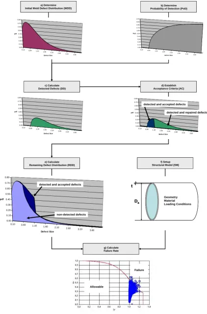
The general evaluation process used represents a combination of statistical methods and probabilistic fracture mechanics using an appropriate structural model. The principal flow diagram is shown in Fig. 1.

(3)

Fig. 1 Principal Procedure

a) Determine

Initial Weld Defect Distribution (WDD)

b) Determine Probability of Detection (PoD)

0.10 0.60 1.10 1.60 2.10 2.60 3.10 3.60 0.00 0.10 0.20 0.30 0.40 0.50 0.60 0.70 0.80 pdf Defect Size

0.10 0.60 1.10 1.60

2.10 2.60 3.10 3.60 P 0.00 0.10 0.20 0.30 0.40 0.50 0.60 0.70 0.80 0.90 1.00 PoD

De fect Size

c) Calculate Detected Defects (DD)

0.10 0.60 1.10 1.60 2.10 2.60 3.10 3.60 0.00 0.10 0.20 0.30 0.40 0.50 0.60 0.70 0.80 pdf Defect Size d) Establish Acceptance Criteria (AC)

0.10 _0.60

1.10 1.60 2.10 2.60 3.10 3.60 0.00 0.10 0.20 0.30 0.40 0.50 0.60 0.70 0.80 pdf Defect Size

detected and repaired defects detected and accepted defects

0.10 0.60 1.10 _1.60

2.10 2.60 _3.10 3.60 0.00 0.10 0.20 0.30 0.40 0.50 0.60 0.70 0.80 pdf Defect Size non-detected defects detected and accepted defects

e) Calculate Remaining Defect Distribution (RDD)

t

Da

f) Setup Structural Model (SM)

Geometry Material Loading Conditions g) Calculate Failure Rate Allowable Failure a) Determine Initial Weld Defect Distribution (WDD)

a) Determine Initial Weld Defect Distribution (WDD)

b) Determine Probability of Detection (PoD)

0.10 0.60 1.10 1.60 2.10 2.60 3.10 3.60 0.00 0.10 0.20 0.30 0.40 0.50 0.60 0.70 0.80 pdf Defect Size

0.10 0.60 1.10 1.60

2.10 2.60 3.10 3.60 P 0.00 0.10 0.20 0.30 0.40 0.50 0.60 0.70 0.80 0.90 1.00 PoD

De fect Size

c) Calculate Detected Defects (DD)

0.10 0.60 1.10 1.60 2.10 2.60 3.10 3.60 0.00 0.10 0.20 0.30 0.40 0.50 0.60 0.70 0.80 pdf Defect Size d) Establish Acceptance Criteria (AC)

d) Establish Acceptance Criteria (AC)

0.10 _0.60

1.10 1.60 2.10 2.60 3.10 3.60 0.00 0.10 0.20 0.30 0.40 0.50 0.60 0.70 0.80 pdf Defect Size

0.10 _0.60

1.10 1.60 2.10 2.60 3.10 3.60 0.00 0.10 0.20 0.30 0.40 0.50 0.60 0.70 0.80 pdf Defect Size

0.10 0.60 1.10 _1.60

e) Calculate Remaining Defect Distribution (RDD)

e) Calculate Remaining Defect Distribution (RDD)

t

Da

t

Da

f) Setup Structural Model (SM)

(4)

Using Monte Carlo simulation the defects are randomly selected from this probability density function and the probability of detection (PoD) is calculated based on a mean PoD curve representing the quality of the NDT-method to be investigated. An example for a typical PoD curve is given in Fig. 1b).

Based on the two distributions mentioned above it can be determined randomly, whether is defect is detected or not. Especially the distribution can be calculated for those defects detected (see Fig. 1c) and those defects not detected. Here it is necessary to introduce the sizing performance of the NDT-methods to be investigated. This means to have a statistical assessment regarding the quality, which with a certain height or length measured by a certain methodology can be assumed. Then, the defects detected are assessed in combination with a certain acceptance criteria to be applied. Then all defects to be rejected by the acceptance criteria are assumed to be repaired. Those ones not rejected will remain in the component (compare Fig. 1d).

Based on the above mentioned steps, the distribution of those defects can be calculated, which will remain in the component either they were not detected or they were detected, but assessed to be acceptable due to the established acceptance criteria. Such a distribution is plotted in Fig. 1e.

This distribution is then the basis for the probabilistic failure assessment in the second step. In this step, it is necessary to create a suitable mechanical model, representing the most important boundary conditions, basically regarding influences resulting from geometry, material, loading conditions, etc. (compare Fig. 1f). Also here it is necessary to discuss the relevancy of deviation from those values usually used for a calculation, neither it can assumed to be conservative or if it is may be necessary to assume distributions like a log-normal distribution for a certain material value.

Combining the numerical model with the calculated distribution of those cracks still present in the component the assessment can be performed whether one of those defects is critical or not. Also for this purpose a Monte Carlo simulation is used by randomly picking a possible defect out of the distribution to be assessed. In Fig. 1g the assessment is shown. The circles demonstrated the results for all those cracks picked and assessed in the two criteria diagram according e.g. to API 579 (2000), BS 7190 (2000), FKM-Richtlinie (2001), SINTAP (1999). All those defects resulting in a point outside the acceptable line are critical. By dividing those defects calculated as critical by the total sum of defects assessed during the sampling procedure the failure rate or probability of failure can be determined as well as some other results created by the entire procedure using additional counters for e.g. numbers of undetected and acceptable defects.

Entirely, the following results can be created by the procedure described:

; Probability of failure or failure rate

; Rate for detected defects

; Repair rate

; Rate for non detected and rejectable defects

; Rate for non detected and acceptable defects

; Rate for correctly and incorrectly accepted/rejected defects.

It should be mentioned that for special tasks or when assessing a specific NDT method some refinements are necessary to be implemented in the principal scheme shown in Fig. 1. So, e. g. for assessing radiography, it is additionally necessary to characterize the defects, whether they are assumed to be cracks or not.

3. INPUT DATA

Summarizing the steps mentioned the following input data is required for the procedure described above:

1. WDD (Initial Weld Defect Distribution), which is a statistical distribution representing the defects populating the welds to be assessed after the production process

2. PoD (Probability of Detection), representing the performance of a special NDT-technique to detect a defect dependent on defect type, size, and orientation.

3. SP (Sizing Performance), representing the quality of sizing a defect in height and length 4. AC (Acceptance Criteria), to be applied either from a code or by specification

5. (SM) Structural Model, representing a close to reality model regarding geometry, material, and loading conditions

(5)

3.1 Initial Weld Defect Distribution (WDD)

The starting point for the analysis is to agree on a specific distribution of defects, which are present in the structure after the manufacturing process. This population basically depends on the manufacturing process itself (e.g. the welding procedure used) but also of course on the quality of the execution. In KINT, 2004 a good literature review on initial defect distribution is provided.

Herein, the distinction between defects caused by ‘workmanship’ and ‘technological’ issues is made. The first ones are e.g. porosity, inclusions lack of fusion, undercut, etc. while the latter includes hot cracking; reheat cracking, hydrogen induced cold cracking, etc. It is also stated that investigations have demonstrated that basically most of the unacceptable defects are ‘workmanship’ defects, occurring in a random manner. Therefore they can be described in a statistical way.

Due to the fact that usually NDT-methods are used to assess the defects in a certain probe or specimen, fewer defects have been observed in the small defect size. So some investigators suggest exponential distribution while others prefer two or three parameter Weibull distributions. Due to the fact that very small defects are negligible for the fracture mechanic assessment, it should not be not within the focus when determining the relevancy of a certain distribution to be used.

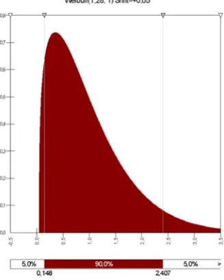
In KINT, 2004 as well as in TOFDPROOF, 2005, the defect distributions were assumed as a three parameter Weibull function. The parameters for embedded and surface breaking defects are given for manual welding as well as for automated welding with mean values. Upper and lower bounds are given as well. The basic description for the probability density function is:

where α, β, γ are the Weibull parameters. An example for the mean distribution for embedded defects caused by automated welding is drawn in Fig. 2.

Fig. 2 Initial Weld Distribution (mean, embedded, automated welding)

3.2 Probability of Detection (PoD) and Sizing Performance (SP)

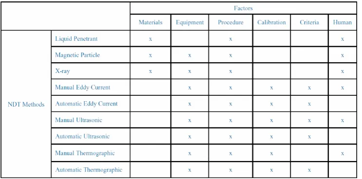
The probability of detection curve (PoD curve) is the established and more or less accepted metric for characterizing the capability of a NDT-procedure. However, it is a challenging task to establish a reliable PoD curve for a particular application, as it depends on a large variety of parameters. In the following Table 1 an overview is given of the most important influence factors for some NDT procedures (compare also NDE Capability Data Book (1997) and Jovanovic, Balos, Kauer (2003)):

)

(

)

/

)

((

1 ( )

) (

β

α γ β

α

γ

α

β

₋ −

−

∗

−

∗

=

a

e

(6)

Table 1 Dominant Sources of Variance in NDT Procedure Application

However, also in combination with the development and the application of new general inspection strategies (see e.g. RIMAP, 2004), it is very important to have knowledge regarding the strength and the weakness of a certain NDT methodology and this not only in a qualitative but in a quantitative manner.

Reference data can be found in projects like PISC (project on inspection of steel components for nuclear components) NORDTEST (a series of Scandinavian projects on fundamental issues in NDE), NIL (a series of Dutch projects on fundamental issues in NDE). More information and the full references of the mentioned projects are provided in Visser (2002). When evaluating data, whether specially created or coming from literature, it is necessary to discriminate between:

; TRUE POSITIVE SIGNAL (TP)

Defect found when a defect is present

; FALSE POSITIVE SIGNAL (FP)

Defect found when no defect is present

; FALSE NEGATIVE SIGNAL (FN)

No defect found when a defect is present

; TRUE NEGATIVE SIGNAL (TN)

No defect found when no defect is present

Based on this information, PoD and the probability of false calls (PoFC) can be expressed as:

FP

TN

FP

PoFC

and

FN

TP

PoD

+

=

+

=

With this definition statistical distributions can be created either based on simple hit/miss data or by so called a-hat data, where the NDT signal response is considered to be the perceived defect size. For more information see e.g. NDE Capability Data Book (1997). The statistical evaluation usually uses cumulative lognormal, log logistic or Weibull distributions to describe the PoD curve.

In the TOFDPROOF project (2005) round robin tests were performed and the data were analyzed to create the PoD curves. In this project the three parameter cumulative Weibull curve was found to fit best the experimental data as it is also documented in KINT (2004). The mathematical expression is

β α γ)/ ) ((

1

)

(

a

=

−

e

− a−

F

,

(7)

Fig. 3 PoD Curve (TOFDPROOF, 3-parameter Weibull, alpha=0.69, beta=0.65,

gamma=0.8)

Values for the Weibull parameter for radiography, TOFD, as well as for manual and automatic ultrasonic testing are summarized and documented in KINT (2004) and Jovanovic, Balos (2005).

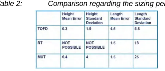
After having detected a defect, it is necessary to size the flaw and evaluating the results with respect to the acceptance criteria (compare Fig. 1d). Looking at the sizing capabilities of each NDT method, the deviations within the application of a particular methodology can be expressed in a statistical way by mean error and standard deviation. However, there are also basic differences between the NDT-methods in sizing a defect. So e.g. on a radiographic film it is only possible to determine the length and/or width of a defect, while by applying TOFD or UT, also the height dimensions can be determined. In the following Table 2 the values found within the TOFDPROOF project are plotted for RT, MUT and TOFD.

Table 2:

Comparison regarding the sizing performance

3.3 Acceptance Criteria (AC)

After a defect has been detected by a certain technique, its dimensions or some other technique-dependant characteristic signals are to be compared with the acceptability limits given in the applicable code or in an agreed specification. In Europe, the hierarchy in assessing welds during pressurized equipment fabrication is the following Figure 4.

When looking for existing acceptance criteria for TOFD, the Dutch Norm NEN 1822 or ASME Code Case 2235 can be used. However, EN 12062 provides three levels of quality (stringent, intermediate, moderate), which also should be present in the acceptance criteria or the NDT method, for example EN 12517 for RT (acceptance levels 1, 2, and 3).

Therefore, the European acceptance criteria for TOFD also will have 3 levels for acceptance to address different values of quality. The proposed acceptance criteria are given in van der Spek, Kauer, Verkooijen (2005). It is strictly recommended to ensure that the acceptance criteria should be involved in the entire process, including NDT system, procedure and operator qualification.

0 0.1 0.2 0.3 0.4 0.5 0.6 0.7 0.8 0.9 1

0 1 2 3 4 5 6

Defect Height [mm]

P

o

D

[-] PoD Curve_TOFD

(8)

Fig. 4 Assessment of welds during pressurized equipment fabrication (EN 13445-5)

After having applied the PoD combined with the statistical description of the sizing performance to the initial weld distribution, the consequences regarding the failure rate is given by the statistical description of the distribution of all defects which are remaining in the component after inspection and repair according to an acceptance criteria (compare Fig. 1e).

3.4 Evaluation Process and Structural Model

Due to the fact that all acceptance criteria and also the way they have been established are focused on the evaluation during the fabrication process, they cannot consider special operational applications. However, there is a difference the consequence caused by a particular defect, e.g. depending on the loading conditions to be expected, basically static or dynamic, which can cause considerable defect growth during operation.

To assess the influence of the calculated defect distribution after inspection and repair on the structural integrity of a certain component, it necessary to establish a reasonable model and technique, especially with respect to geometry, material, and loading conditions.

While weld deficiencies like offset or undercut can be assessed in detail by using standard structural mechanic techniques (like Finite-Element Analysis), it necessary to install Fitness for Purpose / Fitness for Service techniques to evaluate volumetric or planar defects, like slag inclusion, porosity, cracks, etc. (see e.g. Kauer, Beukelmann (2004)). These techniques are described in various codes (e.g. German Nuclear Code KTA, ASME Section XI, API 579, BS 7910, SINTAP, FKM).

For steel, the two criteria approach as documented e.g. in SINTAP is widely accepted in the meantime. Here, both brittle fracture and plastic collapse aspects are considered. The result for an actual evaluation point is plotted in the so called FAD (Failure Assessment Diagram) and compared to a curve representing the border between allowable and critical values. An example for such a plot is given in Figure 5, also showing the principal influence of cyclic loading.

Fig. 5 FAD Diagram (Two criteria approach)

EN ISO 5817

Specifies quality levels based upon real defct types and dimensions

EN 12062

Interface between quality levels and indications found by an NDT method

NDT Method Procedure Acceptance Criteria

VT EN 97 EN 25817

RT EN 1435 EN 12517

UT EN 1714 EN 1712

PT EN 571-1 EN 1289

MT EN 1290 EN 1291

TOFD XPCEN/TS14751 under construction

EN ISO 5817

Specifies quality levels based upon real defct types and dimensions

EN 12062

Interface between quality levels and indications found by an NDT method

NDT Method Procedure Acceptance Criteria

VT EN 97 EN 25817

RT EN 1435 EN 12517

UT EN 1714 EN 1712

PT EN 571-1 EN 1289

MT EN 1290 EN 1291

TOFD XPCEN/TS14751 under construction

Safety Crack Growth for

10.000 Cycles:

Allowable Area

Critical Area

Safety Crack Growth for

10.000 Cycles:

Allowable Area

(9)

Within the procedure shown in Fig. 1, the described evaluation procedure is continuously passed through for all samples of the Monte Carlo Simulation. After this, the failure rate can be determined by dividing all samples ending up in the critical area by total number of samples evaluated.

It is obvious that the geometry, the material and the loading conditions for the structural should best fit the conditions in reality. Regarding the material values, basically the fracture toughness is of importance. It should be mentioned that also for this or other values, like yield strength or geometrical values, statistical distributions can be used to describe the reality (e.g. log-normal distribution for the fracture toughness). Often however, conservative but tangible assumptions yield to reasonable results as well.

It is important that the structural model contains all relevant loading conditions to be expected during the entire service life. Also geometrical deviations while the component is in operation, e.g. wall thinning caused by corrosion or erosion, can be considered if reasonable.

4. APPLCIATION EXAMPLE

In the following an example is given to demonstrate the applicability of the described method for comparing the performance of two NDT methodologies (RT and TOFD) for a certain range of components (pipe DN 900 with internal pressure and bending moment and various thicknesses).

4.1 Input Data and Boundary Conditions

The pipe under investigation has an outside diameter of 914 mm and the thickness range to assess is 6 mm, 15 mm, and 36 mm.

Material is P265GH and the relevant material data is: Modulus of Elasticity: 2.12E+5 MPa, Yield Strength: 265 MPa, Tensile Strength: 410 MPa, and Fracture Toughness: 1750 N/mm^3/2.

The two loading conditions internal pressure and internal pressure combined with an external bending moment to be considered were determined on the basis of 100% of the allowable taking into account a safety factor of 1.1.

The evaluation considers embedded and surface breaking defects. The remaining defect distributions after inspection and repair were calculated for RT and TOFD based on the initial weld distributions for automated welding (3-parameter Weibull distributions with values according to KINT (2004)) and PoD curves and sizing performance as described in TOFDPROOF (2005). The acceptance criteria for RT is derived from EN 12517 Level 1, while for TOFD all three levels for the acceptance criteria as proposed in TOFDPROOF (2005) were evaluated.

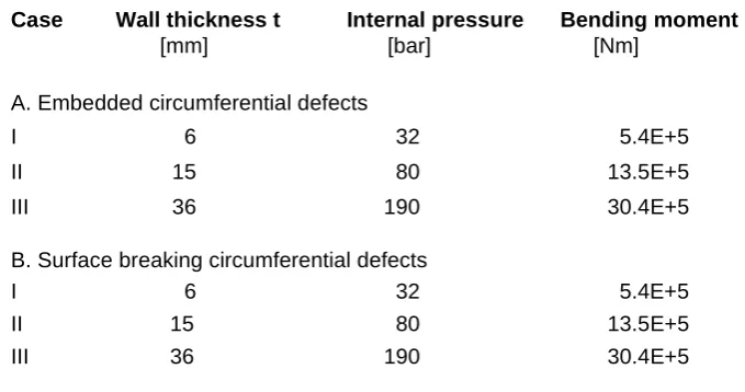
With this information basically 6 different cases must be considered each of them evaluated by RT Level 1 and TOFD Level 1, 2, and 3. An overview of the 6 cases A.I to B.III is given in the following Fig. 6.

Fig. 6 Cases to be considered

Case Wall thickness t Internal pressure Bending moment

[mm] [bar] [Nm]

A. Embedded circumferential defects

I 6 32 5.4E+5

II 15 80 13.5E+5

III 36 190 30.4E+5

B. Surface breaking circumferential defects

I 6 32 5.4E+5

II 15 80 13.5E+5

(10)

4.2 Results

In Figure 7, the distributions for the remaining defects after inspection and repair (compare Fig. 1e) can be compared for RT and TOFD and the thickness 36 mm, each of them considering the level 1 acceptance criteria. As can be seen e.g. for 2 mm, for RT there are more defects remaining in the structure.

Fig. 7 Weibull Distribution for all defects remaining in the structure after inspection

and repair

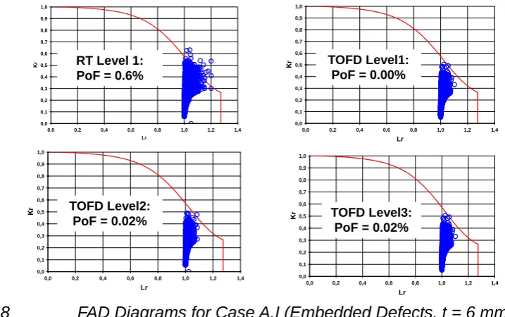
In Figure 8, the results of the Monte Carlo simulation are shown, demonstrating the effect of a certain failure out of the remaining failure distribution after inspection and repair. So, for RT there are several assessment points outside the acceptable area and the probability of failure is calculated to end up at 0.6%, whereas the failure rate for TOFD is lower even for the lowest acceptance level 3.

Fig. 8

FAD Diagrams for Case A.I (Embedded Defects, t = 6 mm) showing

10.000 trials

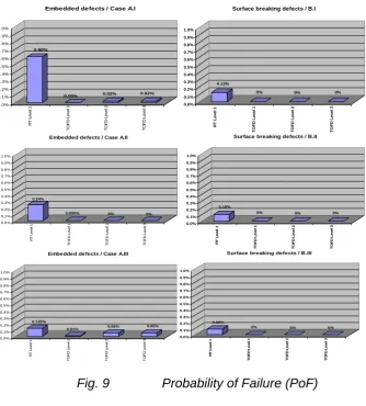
In Figure 9, the probabilities of failure (PoF) for all six cases are shown. As an obvious result it can be seen that the failure rates for the TOFD procedure are much lower than for RT for all six cases considered. Even for the level 3 acceptance criteria the highest failure rate is at 0.06% for case A.III, whereas for most of the cases the failure rate for TOFD is around 0%.

0 1,00 0,20 0,40 0,60 0,80

0 2,00 4, 00 6, 00 8, 00 10, 00

Probability Density Function

Tim e, (t)

f(

t)

27. 04. 2005 09: 41 abc abc W eibull D at a 1 W3 R R 3 - SR M M ED F =8332 / S=0

α= 0.813

β= 1.328

γ= 0.050

0 1,00 0,20 0,40 0,60 0,80

0 2, 00 4, 00 6, 00 8, 00 10, 00

Tim e, (t )

f(

t)

27.04. 2005 09: 45 abc abc W eibull D at a 1 W3 R R 3 - SR M M ED F =9999 / S=0

α= 0.990

β= 1.300

γ= 0.050

TOFD Level 1 ( t = 36 mm) RT Level 1 ( t = 36 mm)

0 1,00 0,20 0,40 0,60 0,80

0 2,00 4, 00 6, 00 8, 00 10, 00

Tim e, (t)

f(

t)

α= 0.813

β= 1.328

γ= 0.050

0 1,00 0,20 0,40 0,60 0,80

0 2,00 4, 00 6, 00 8, 00 10, 00

Tim e, (t)

f(

t)

α= 0.813

β= 1.328

γ= 0.050

0 1,00 0,20 0,40 0,60 0,80

0 2, 00 4, 00 6, 00 8, 00 10, 00

Tim e, (t )

f(

t)

α= 0.990

β= 1.300

γ= 0.050

0 1,00 0,20 0,40 0,60 0,80

0 2, 00 4, 00 6, 00 8, 00 10, 00

Tim e, (t )

f(

t)

α= 0.990

β= 1.300

γ= 0.050

TOFD Level 1 ( t = 36 mm) RT Level 1 ( t = 36 mm)

0,0 0,1 0,2 0,3 0,4 0,5 0,6 0,7 0,8 0,9 1,0

0,0 0,2 0,4 0,6 0,8 1,0 1,2 1,4 Lr 0,0 0,1 0,2 0,3 0,4 0,5 0,6 0,7 0,8 0,9 1,0

0,0 0,2 0,4 0,6 0,8 1,0 1,2 1,4 Lr

RT Level 1: PoF = 0.6%

TOFD Level1: PoF = 0.00%

TOFD Level2:

PoF = 0.02% TOFD Level3:

(11)

If the task was to demonstrate the same level of safety when substituting RT by TOFD, it can be summarized that is true for the application considered and especially for the acceptance criteria chosen. Additionally it can be stated that the acceptance according to TOFD level 3 is sufficient enough.

Fig. 9

Probability of Failure (PoF)

5. SUMMARY

For this purpose a procedure is presented, which is a combination of statistical methods and fracture mechanic assessment. With the knowledge of the distribution of all defects remaining in a certain structure after inspection and repair, the failure rate can be calculated by applying Monte Carlo simulation on the fracture mechanic assessment for particular structures. With the output of this procedure, answers can be given to the above mentioned question.

NOMENCLATURE

NDT Non-destructive testing PoD Probability of detection RT Radiographic testing

(M)UT (Manual) ultrasonic testing

0.60%

0.00% 0.02% 0.02%

0.0% 0.1% 0.2% 0.3% 0.4% 0.5% 0.6% 0.7% 0.8% 0.9% 1.0% R T Lev el 1 T O F D Lev el 1 T O F D Lev el 2 T O F D Lev el 3

Embedded defects / Case A.I

0.24%

0.000% 0% 0%

0.0% 0.1% 0.2% 0.3% 0.4% 0.5% 0.6% 0.7% 0.8% 0.9% 1.0% RT L e v e l 1 TO FD L e v e l 1 TO FD L e v e l 2 TO FD L e v e l 3

Embedded defects / Case A.II

0.125%

0.01% 0.05% 0.05%

Embedded defects / Case A.III

0.13%

0% 0% 0%

0.0% 0.1% 0.2% 0.3% 0.4% 0.5% 0.6% 0.7% 0.8% 0.9% 1.0% R T Le v e l 1 TOFD Le v e l 1 TOFD Le v e l 2 TOFD Le v e l 3

Surface breaking defects / B.I

0.10%

0% 0% 0%

0.0% 0.1% 0.2% 0.3% 0.4% 0.5% 0.6% 0.7% 0.8% 0.9% 1.0% RT L e v e l 1 T O FD Le v e l 1 T O FD Le v e l 2 T O FD Le v e l 3

Surface breaking defects / B.II

0.09%

0% 0% 0%

0.0% 0.1% 0.2% 0.3% 0.4% 0.5% 0.6% 0.7% 0.8% 0.9% 1.0% RT L e v e l 1 TO FD Le v e l 1 TO FD Le v e l 2 TO FD Le v e l 3

Surface breaking defects / B.III

0.60%

0.00% 0.02% 0.02%

Embedded defects / Case A.I

0.24%

0.000% 0% 0%

0.0% 0.1% 0.2% 0.3% 0.4% 0.5% 0.6% 0.7% 0.8% 0.9% 1.0% RT L e v e l 1 TO FD L e v e l 1 TO FD L e v e l 2 TO FD L e v e l 3

Embedded defects / Case A.II

0.125%

0.01% 0.05% 0.05%

Embedded defects / Case A.III

0.13%

0% 0% 0%

0.0% 0.1% 0.2% 0.3% 0.4% 0.5% 0.6% 0.7% 0.8% 0.9% 1.0% R T Le v e l 1 TOFD Le v e l 1 TOFD Le v e l 2 TOFD Le v e l 3

Surface breaking defects / B.I

0.10%

0% 0% 0%

0.0% 0.1% 0.2% 0.3% 0.4% 0.5% 0.6% 0.7% 0.8% 0.9% 1.0% RT L e v e l 1 T O FD Le v e l 1 T O FD Le v e l 2 T O FD Le v e l 3

Surface breaking defects / B.II

0.09%

0% 0% 0%

0.0% 0.1% 0.2% 0.3% 0.4% 0.5% 0.6% 0.7% 0.8% 0.9% 1.0% RT L e v e l 1 TO FD Le v e l 1 TO FD Le v e l 2 TO FD Le v e l 3

(12)

TOFD Time of flight diffraction PoF Probability of Failure FAD Failure assessment diagram pdf Probability density function

REFERENCES

TOFDPROOF (2005), “Effective Application of TOFD Method for Weld Inspection at the Manufacturing Stage of Pressure Vessels”, Commission of the European Communities GROWTH Project G6RD-CT-2001-00626

KINT (2004), Guideline for the determination of acceptance criteria for defects in pipeline girth welds”, June 14, 2004

EN 12517 (2003), “Non-destructive examination of welds – Radiographic examination of welded joints in steel – Acceptance levels”, 2003-01

API RP 579 (2000), “Fitness for Service”, American Petroleum Institute, Jan. 2000

British Standard 7910 (2000), “Guide on methods for assessing the acceptability of flaws in metallic structures”, BSI, 10-2000

FKM-Richtlinie (2001), „Bruchmechanischer Festigkeitsnachweis für Maschinenbauteile“, VDMA Verlag, 2001

SINTAP (1999), “Structural Integrity Assessment Procedure” European Union Project, Brite Euram Programme, 1999

NDE Capabilities Data Book (1997), “Nondestructive Evaluation Capabilities Data Book”, Texas Research Institute Austin Inc., Nov. 1997

Jovanovic, A., Balos, D., Kauer, R. (2003), “Treatment of Uncertainties in Determination of Acceptance Criteria for Ultrasonic Testing“, UNCERT-AM Conference on Management of Uncertainties in Mechanical Testing and Inspection, MPA-Stuttgart, Germany, October 8, 2003

RIMAP (2004), “Risk-Based Inspection and Maintenance Procedures for European Industries”, Commission of the European Communities GROWTH Project G1RD-CT-2001-03008

Visser, P.W. (2002), “POD/POS curves for non-destructive examination”, HSE Report, 2000/18

Jovanovic, A., Balos, D. (2005), “What is the performance of TOFD? Comparison with conventional methods”, TOFDPROOF Seminar, Paris-Villepinte, March 18, 2005

Van der Spek, E. Kauer, R., Verkooijen, J. (2005), “Acceptance Criteria – Proposal for a European Standard – Links to EN ISO 5817”, TOFDPROOF Seminar, Paris-Villepinte, March 18, 2005

Kauer, R. Beukelmann, D. (2004), “Gesamtheitliche Bewertung gleichzeitig auftretender Einzelfehler”, SLV-Tagung, München, Feb. 2004.

KTA-Regeln 3201.4/3211.4, „Wiederkehrende Prüfungen und Betriebsüberwachung“