Predicting Harmonic Centrality In Aodv For
Wireless Sensor Networks Using Machine
Learning
Pallavi R., Vishal V., Tushar Sharma, G.C. Banu Prakash
Abstract - The Ad Hoc On-Demand Distance Vector routing protocol is the ideal protocol for routing in dense wireless networks. The metrics used to evaluate centrality for such networks include betweenness, closeness, degree, harmonic etc. The harmonic centrality is a better metric at leadership recognition. The authors propose an optimal machine learning approach to predict the harmonic centrality for each node based on few network parameters. The hypothesis that the distance from the source to destination contributes to the harmonic value is investigated. Regression models and Artificial Neural Networks were used to find the equation that fits the feature columns with minimum error. From the experiments, the authors concluded that the distance (closeness) does not contribute significantly towards leadership recognition in the network. Among the various approaches experimented with to predict the harmonic centrality, linear models showed a better fit and minimum error even in the case of scaling up the network.
Index Terms - AODV, Harmonic Centrality, Regression, Neural Networks
————————————————————
1
INTRODUCTION
he AODV routing protocol is used for in dense wireless ad hoc networks. Such Wireless Sensor Networks (WSN) can self-deploy rapidly and use the protocol to scale on demand. Hence, they can be used in self-scalable applications with rapid growth potential, especially in large scale social networks. This could also lead to a concern regarding the uncertainty in the topology especially when the scale is unprecedented. Thus there is a need for predictive metrics to identify the critical nodes that ensure a connection between clusters of nodes. Such nodes also known as leaders can be discerned effectively using harmonic centrality over closeness and betweenness. Computing the harmonic values can be computationally intensive and uncertain owing to the steep scalability index during the network growth. Hence, a predictive model that can predict the harmonic or h-values with minimum error percentage can enable monitoring of the system. The paper shows the NS2 simulation of a large network in which nodes range from 100 to1000 in number.
Each node is characterized by its throughput, delay, energy, neighbor count, neighbors, the average number of hops, and the destination node. Our investigation is based on the hypothesis that the ―closeness factor‖ or vicinity plays a statistically significant role in predicting the H value. The protocol attempts to predict the H value using various machine learning techniques to find an equation that predicts the value with the least absolute error.The rest of the paper is organized as follows, Section I contains the introduction of the problem, Section II contain the related work, Section III describes the methodology used, Section IV describes results and discussion, Section V concludes the key factors of the paper with conclusion and also enhances the future directions.
2
RELATED
WORK
Recent papers [16] based on AODV protocol deals with the study of the creation of the dataset and the evaluation metrics for the Harmonic centrality values which are useful for the computation of the distance vector parameters for AODV protocol. D. Bhattacharyya, T.-H. Kim and S. Pal [1] suggest the idea of transferring the data based on a cluster approach for the wireless network’s path detection. D. Acemoglu, G. Como, F. Fagnani, and A. Ozdaglar [2] deal with the study of a tractable opinion dynamic model that generates long-run disagreements and persistent opinion fluctuations. The model involves an inhomogeneous stochastic gossip process of continuous opinion dynamics consisting of regular agents and stubborn agents that shows the uncertainty in the growth of the network. N. E. Friedkin [3] gives a brief description of the calculation of the centrality example and helps to obtain one for the AODV protocol which helps for the optimal path detection. M. Marchiori and V. Latora [4] give a brief about the use of social networks in great depth and helps with the study of energy and throughput which is also used by our model. A. Bavelas [5] deals with the connectivity of the group networks i.e. connectivity when many tasks are associated with the same network and the throughput is altered and optimal paths are chosen for the efficient implementation of the model. Xiaodong Wang, Daxin Zhu [6] suggests the use of A* algorithm for the dynamic allocation of the total distance values for the easier computation of the model and limit the GPU usage of the model for calculating the distance from one hop to another. [7] Suggests the use of the linear regression T
___________________________
Manuscript received September 2, 2019. The authors declare that there is no conflict of interest regarding the publication of this paper.
Pallavi R. is a Faculty of Computer Science and Engineering,Sir M Visvesvaraya Institute of Technology, Bangalore, India, [email protected]
Vishal V. is with Department of Computer Science and Engineering,Sir M Visvesvaraya Institute of Technology, Bangalore, India, [email protected]
Tushar Sharma is with Department of Computer Science and Engineering, Sir M Visvesvaraya Institute of Technology, Bangalore, India, [email protected]
statistical model which uses the concepts of equation creations from the obtained model. [8] Suggests the selection process of the linear regression models with the use of probabilistic values found by the parameters of the dataset. [9] Uses the concept of polynomial regression models and the limitations of the same, it helps for the feature analysis of the polynomial equations. [10] Discusses the Support Vector Machines and the recent advancement to the SVMs and deals with the conditions requirements associated to the SVMs. [11] briefs about the use of decision tree for the dataset based on the variation between values associated to Harmonics. [12] Summarizes the use of Random Forest Regression which is considered to be the best low computational model but does not implement in this case due to lack of dataset for train and test sets. [13] refers to the use of Neural Networks use in the medical dataset which can also be implemented in the dataset but the time and space computation will be high as compared to the random forest regression.
3
METHODOLOGY
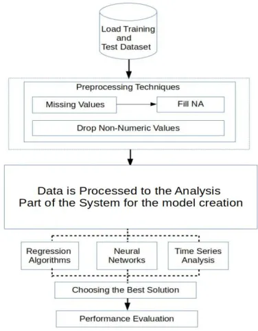
The approach to investigate the above hypothesis is based on the computation of p-values(Probabilistic values) which help to find the significance of the feature (among various features) in predicting the H value. The coefficient of the feature column describes the significance level of parameters and that in turn describes the contribution of the parameter towards the prediction. In order to start with a dataset, authors here have run AODV on the network under study and recorded the various features as shown in the table 1. With large data available for study, data learning algorithms can be used to acquire the underlying pattern of the network.The paper discusses various machine learning techniques to create the desired model for the use-case and tuned the hyperparameters of those which can be deployed on a large scale with minimal computational overload. Most neural network models in deployment have very good accuracy but are quite large and constitute a time delay to generate an inference. Hence a tradeoff with the time delay and accuracy also plays a role in choosing the machine learning model. Figure 1 depicts the machine learning pipeline where the dataset created is the test dataset. The model processes the dataset in various stages and finally helps in evaluating the performance of the network.
Fig.1. Machine Learning Pipeline
3.1 PRE-PROCESSING THE DATA
Fig.2.Social Network Node Simulation of 100 nodes
3.2 ANALYZING THE DATASET
The analysis of data is the next step in the data pipeline. It is done on the initial assumptions of the completeness of the data. We have tried various statistical and machine learning techniques to obtain the equation of best fit. They include:
3.2.1MULTIPLE LINEAR REGRESSION
Multiple Linear Regression is used to explain the relationship between multiple independent variables and the dependent variable. The variables in the relationship are considered to be linearly separable and the coefficients are computed to obtain the line of best fit. This linear approach consists of four nuances:
All-In Training: This approach deals with fitting the model on the entire dataset. This method showed heavy over fitting and the inability to generalize well on many of the instances as the hyper parameter tuning did not improve the model significantly.
● Threshold Pruning: This approach deals with the removal of least contributing parameters and uses only the essential ones. These are chosen based on a threshold value set to prune away parameters with a coefficient lesser the threshold value. These are repeated for the calculated p-values (Probabilistic values) of the statistical model as well to cross-reference the initial hypothesis.
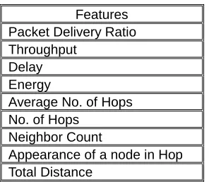
TABLE I: FEATURE COLUMNS IN THE PRE-PROCESSED DATA
Features Packet Delivery Ratio Throughput
Delay Energy
Average No. of Hops No. of Hops
Neighbor Count
Appearance of a node in Hop Total Distance
● Intercept Buffer: This approach deals with the concept of establishing a relation along with the intercept to minimize the total absolute error. This increases the number of feature columns to train the model, but the tradeoff is relatively small and hence is efficient. This buffer value accounts for the errors and hence finds the line of best fit with lesser standardized error. ● Ensemble Training: In this approach, an ensemble of
models is used to make a prediction and the top k values are considered and the mean of these predictions are considered. The training is parallelized and the different models each use a different initialization strategy. The ensemble of models showed a high combined accuracy. But, this approach is computationally intensive and does not always give an accurate result.
3.2.2 POLYNOMIAL REGRESSION
Polynomial regression is used to explain the relationship between multiple independent variables and the dependent variable in a nonlinear manner. The dependent variable is mapped as an nth degree variable and is used to model a nonlinear relationship to find the line of best fit. It is denoted as E(y |x). This approach does not align well with our hypothesis as the polynomial relation skews the available data as the distance value cannot be scaled and thus is biased to have a much smaller coefficient.
(i)
3.2.3 SUPPORT VECTOR REGRESSION
A support vector regressor deploys a nonlinear kernel and finds the maximum margin in the data correlating the variables. Thus, a support vector regressor ends up performing a nonlinear regression which as noted above skews our distribution and undermines the contribution of some of the features that cannot be scaled. The kernel trick represents the model as a combination of training points rather than as an expression. Thus, the nonlinear mapping brings a nonlinear expression as a mapping.
∑ ( ) * ( ) ( )+ (ii)
3.2.4 ARTIFICIAL NEURAL NETWORK
Fig. 3. Neural Network Architecture
The model trained used 3 Dense (Fully-Connected) layers with Rely activation at each layer and a Mean Squared Error (MSE) as the loss function. The SGD (Stochastic Gradient Descent) optimizer was a natural choice and implies that the neural network updates its weights after every training example. We used the Tensor flow library and high level keras that ships with eager execution by default (Tensor flow 2.0). From all our hyper parameter tuning to improve the accuracy of the model we noticed over fitting especially due to variability in the data.
4
RESULTS
AND
DISCUSSION
The paper tries to bring in the best data learning technique used to understand the best-fit pattern for deploying the nodes. Rigorous testing were executed for various techniques using the R tool. The various machine learning techniques used to predict the harmonic centrality values provided a unique insight into the functional mapping of how the distance (closeness index) affects our prediction. Polynomial regression showed that the nonlinear mapping biased the model into undermining the contributions of the unscaled parameters. However, this does not imply that by normalizing the feature, the mapping would have a better significance. This is because one cannot arbitrarily define the extent of the scale factor and the contribution of the values that are not normalized. The polynomial regression model and the support vector regressor (SVR) perform a nonlinear mapping and hence do not provide an accurate representation of our data. The SVR and Polynomial regression showed a high error rate of 26.43% and 22.81% respectively and is consistent with our hypothesis and analysis. The neural network (ANN) showed much promise with the powerful gradient descent optimizer. The input vector’s mapping would be refined by this optimizer but the case of over fitting even with a low learning rate showed that the variability is high and it is difficult to generalize for the AODV protocol data in wireless sensor networks. This also means that considerably large datasets with 1000s of nodes might not be large enough data to find a mapping for using ANNs or deeper neural networks. The neural network showed an error of 16.12% but did not generalize well in predictions. Hence, the paper concludes it as over-fit on the training data despite tuning the hyperparameters.The linear regression models among their different nuances showed the best results for our use case. This is because it forms a linear mapping between the dependent variable and the independent variables. The All-In approach over-fit on the training data
poorly on the withheld validation set. To regularizing effect of pruning some of the feature columns like the energy of the network and the delay showed a slight performance improvement for the regression model and had an error of 10.23% with a better generalization on the validation data. Ensemble training is based on the philosophy that multiple tweaked models can predict better than one. But, the average of the results that are computed could generalize well on the validation set with errors ranging from 21.2% to 9.61%. This is owing to the high variability of the wireless sensor network data, but is a good prediction model as the error on the validation set was lesser. The linear regression model with the intercept buffer showed the best performance for the given data with errors ranging from 5.56% to 14.32% with a much better accuracy on the validation data. Thus, despite the use of ANNs and other complex models, the humble linear regression model showed the best performance with minimum error for the WSN data.
TABLE II: FINAL LINEAR REGRESSION MAPPING
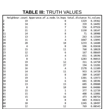
TABLE III: TRUTH VALUES
5
CONCLUSION
The results showed that the use of ANNs, polynomial regression and support vector regression are not apt for the current data set. The linear regression model with the intercept showed the best result in predicting the harmonic centrality values in the AODV routing protocol for wireless sensor networks. The results also show the low value of the coefficient for distance value proving against our hypothesis that closeness index plays a statistically significant role in predicting the harmonic centrality value. Thus, the paper concludes that the closeness index does not contribute in a statistically significant measure and that the linear regression model is a better statistical method in predicting the harmonic value. The future research in this direction would be to consider more parameters like the orientation of the nodes with respect to the sink node and many more to ascertain the importance of harmonic centrality metric in the network.
REFERENCES
[1] V R Sadasivam, Dr K Duraisamy , R Mani Bharathi:‖ Association Rule Mining And Frequent Pattern Mining Applications On Crime Pattern Mining: A Comprehensive Survey‖: International Journal Of Innovative Research In Science, Engineering And Technology Vol. 4, Special Issue 6, May 2015
[2] D. Bhattacharyya, T. H. Kim, S. Pal, ―A comparative study of wireless sensor networks and their routing protocols‖, in Sensors, Vol. 10, No. 12, pp. 10506-10523, 2010 [3] D. Acemoglu, G. Como, F. Fagnani, and A. Ozdaglar,
―Opinion fluctuations and disagreement in social networks‖, Math. Oper. Res., Vol. 38, No. 1, pp. 1–27, Feb. 2013.
[4] N. E. Friedkin, ―Theoretical foundations for centrality measures‖,American Journal of Sociology, Vol. 96, No. 6, pp. 1478–1504, 1991.
[5] M. Marchiori and V. Latora, ―Harmony in the small-worldPhysica A: Statistical Mechanics and its Applications‖, Vol. 285, No. 3, pp. 539 – 546, 2000.
[6] A. Bavelas, ―Communication Patterns in Task-Oriented Groups‖, Acoustical Society of America Journal, Vol. 22, p. 725, 1950.
[7] Xiaodong Wang, Daxin Zhu, ―A Fast Route Planning Algorithm‖, 2012 Spring Congress on Engineering and Technology IEEE, 12 November 2012
[8] Mark Lunt, ―Introduction to statistical modelling: linear regression‖, Rheumatology, Volume 54, Issue 7, July 2015
[9] Zoran Bursac, C Heath Gauss, David Keith Williams, David W Hosmer, ―Purposeful selection of variables in logistic regression'', Source Code for Biology and Medicine,2008
[10]Eva Ostertagova, ―Modelling Using Polynomial Regression‖, Procedia Engineering, 48, 2012
[11]Yingjie Tian, Yong Shi, Xiaohui Liu, ―Recent Advances in Support Vector Machines Research‖, Technological and Economic Development of Economy 18, March 2012 [12]Himani Sharma, Sunil Kumar,―A Survey on Decision Tree
Algorithms of Classification in Data Mining‖, International Journal of Science and Research (IJSR) 5, April 2016 [13]Gerard Biau, ―Analysis of a Random Forests Model‖,
Journal of Machine Learning Research, 13, 2012
[14]Warren S. Sarle, ―Neural Networks and Statistical Models‖, Proceedings of the Nineteenth Annual SAS Users Group International Conference, April, 1994 [15]]K. Stephenson and M. Zelen, ―Rethinking centrality:
Methods and examples‖, Social Networks, Vol. 11, No. 1, pp. 1 – 37, 1989.
[16]Seong-eunYoo, A. M. Cheng, P. K. Chong, T. S. Lopez, and T. Kim, ―Technological advances in wireless sensor networks enabling diverse internet of things applications‖ International Journal of Distributed Sensor Networks, Vol. 14, No. 3, p. 1550147718763220, 2018.