Bimetallic tris-oxalate magnets : Synthesis, structure and properties

BIMETALLIC TRIS-OXALATE MAGNETS:

SYNTHESIS, STRUCTURE AND PROPERTIES

Christopher John Nuttall

University College London

thesis submitted for the degree of Doctor of Philosophy from the University of London

ProQuest Number: U642291

All rights reserved

INFORMATION TO ALL USERS

The quality of this reproduction is dependent upon the quality of the copy submitted.

In the unlikely event that the author did not send a complete manuscript and there are missing pages, these will be noted. Also, if material had to be removed,

a note will indicate the deletion.

uest.

ProQuest U642291

Published by ProQuest LLC(2015). Copyright of the Dissertation is held by the Author.

All rights reserved.

This work is protected against unauthorized copying under Title 17, United States Code. Microform Edition © ProQuest LLC.

ProQuest LLC

789 East Eisenhower Parkway P.O. Box 1346

BIMETALLIC TRIS-OXALATE MAGNETS:

SYNTHESIS, STRUCTURE AND PROPERTIES

by Christopher John Nuttall, of the Royal Institutution London, submitted for the degree of Doctor of Philsophy 1998.

Abstract

In this thesis the series of compounds (cation)M^iFe^^^(ox) 3 {M^ = Mn and Fe, ox = ^2 0 4^"} are studied for cation = NPr4, NBU4, Npent4, PPtu^ A sPh4, PBU4 and PPN. X-ray diffraction reveals all 14 compounds crystallise with layer honeycomb structures. A linear correlation is found for both the inter-layer and the intra-plane unit-cell parameters between analogous MnFe and FeFe compounds. The profiles have been compared to single crystal structure models of (cation)MM'(ox) 3 in the form of partial refinem ent. For cation = N pent4 the powders can be described by the C 2 2 2 (l) Npent4MnHFeH^(ox) 3 single crystal structure (solved at 120K). In the case of cation = NPr4, NBu4 and PBU4, the compounds have found to be bi-phasic containing R3c and P6(3) phases, similar to the R3c NBu4M nCr(ox) 3 and P6(3) NBu4M nFe(ox) 3 single crystal structures. A stacking faulting model, allowing the layer sequence to vary between R3c and P6(3) structures, was found to explain the broadening apparent in the X-ray profiles.

(cation)MHFeHi(ox) 3 {M^ = Mn, Fe} compounds present a variety of magnetic ordering phenomena. (cation)Mn^^Feni(ox) 3 compounds are nominally antiferromagnet w ith Tc's in the range 24-27K. N eutron diffraction experim ents on PPh4(- d2o)MniiFeHi(ox) 3 reveal the magnetic structure to be well explained by antiparallel spin alignm ent along the c-axis with R 3 c m agnetic Shubnikov symmetry. The low temperature uncompensated moments exhibited in the MnFe compounds were reasoned to be the result of sublattice disorder.

Acknowledgements

I would like to thank m y supervisor, Peter Day for his constant encouragement, support, open-mind and guidance throughout my PhD.

I am in d eb ted to C o rin e M ath io n ière w ho w orked in p arallel on the (cation)MHFeHi(ox) 3 compounds and helped greatly in both their synthesis and the purification during my first year.

I would like to thank M ark Green for sharing his sharp insight into solid state structural chemistry and encouraging me to tackle 'impossible' data.

I would like to thank Professor Yakushi and Dr Nakasawa at the I.M.S. (Japan) for much help and support during my stay. Thanks to Hiroshi and Chihoko for making my stay very special and their friendship.

Thanks to Mo Kurmoo for assistance and encouragement early on.

Thanks to Sim on C arling for accom panying me on num erous, som etim es embarrassing. Neutron diffraction experiments and also for some assistance on UNIX computers.

Thanks to Steven Bramwell (my UCL supervisor) and Kosmas Prassides for useful discussions; and again to Kosmas for letting me have-a-first-go at MuSR at PSI.

Thanks to Simon Carling and Dick Visser for their help during the MuSR experiments performed at ISIS.

Thanks to Richard Catlow for letting me use his computers (and his generosity) throughout my PhD - without me even asking.

Table of Contents

CHAPTER 1

I n t r o d u c t i o n ... 17-29

1.1 Overview...17

1.2 Strategies to molecular magnets... 18

1.2.1 Purely molecular magnets... 18

1.2.2 M olecular based magnets with extended lattices... 20

1.3 Scope of the research... 28

CHAPTER 2

M a g n e tic th e o r y ...30-39 2.1 Susceptibility... 30

2.2 Magnetic interactions... 31

2.3 Long range magnetic order... 32

2.3.1 Magnetic model h am iltonians... 32

2.3.2 M olecular field th e o ry ...34

2.3.3 Spin c a n tin g ... 39

CHAPTER 3

E x p e r im e n ta l te c h n iq u e s ...40-61 3.1 D iffraction... 40

3.1.1 Powder X-ray diffraction...42

3.1.2 Neutron diffraction... 42

3.1.3 Powder neutron diffraction instruments... 46

(i) D IB instrum ent... 47

(it) D IA in s tru m e n t... 47

3.1.4 Fitting powder diffraction profiles...49

3.1.5 Diffraction from disordered layer compounds... 52

3.2 M agnetometry...53

3.2.1 Low field DC SQUID measurements...53

3.2.2 High field DC SQUID measurements... 54

3.2.2 Alternating current (AC) magnetometry... 54

3.3 The M uSR technique... 56

CHAPTER 4

Synthesis and structural properties of (cation)MHFeHi(ox

)3

compounds.

... 62-103 4.1 Synthesis and characterisation...62

4.1.1 Synthesis of PPh4(-d2o)MHFei"(ox) 3...65

(i) Preparation o f the Grignard reagent Ph(-d^jMgBr...66

(ii) Preparation o f

PPh

4

(-d

2

o)Br

...

66

(Hi) Preparation o fP P h ^-d2o)Mn^^Fe^^^(ox)s and PPh4(-d2o)Fe^^Fe^^^(ox) 3 67 4.2 Powder X-ray diffraction...6 8 4.2.1 General X-ray profiles and unit cell extraction...6 8 4.3 Structural models... 74

4.3.1 N p e n t4M^^FeHi(ox) 3... 74

4 .3.2 (cation)Mi*Feiii(ox) 3 {cation = NPr^, NBU4, PBU4}... 77

4.3.3 PPh4M "F e"i(o x) 3 and AsPh4M "F ei"(o x) 3...8 6 4 .3 .4 Sample dependence of powder diffraction profiles... 87

4.3.5 (PPN )M "FeH t(ox) 3 compounds...8 8 4.3.6 Attempted preparation of single crystals...90

4.4 Neutron diffraction... 91

C H A P T E R 5

M a g n e tic c h a r a c te r is a tio n o f (cation)M *^Fe*i^(ox) 3 c o m p o u n d s by A C a n d D C SQ U ID m a g n e to m e try ...104-134

5.1 Overview... 104

5.2 Fe^Fe^^^ oxalate salts...104

5.2.1 General behaviour... 104

5.2.2 Compounds with a negative low temperature magnetisation 107 (i) Low fie ld studies... 107

(ii) High fie ld studies... 112

(Hi) A C susceptibility m easurem ents... 119

5.2.3 Compounds with a positive low temperature magnetisation 119 (i) Low fie ld studies... 119

(ii) H igh fie ld studies...124

(Hi) A C susceptibility m e a su rem e n ts...126

5.3 Mn^^Fe^ii oxalate salts... 129

C H A P T E R 6 In v e s tig a tio n o f (cation)Fe^*Fe^^^(ox) 3 c o m p o u n d s w ith lo c al m a g n e tic p r o b e s ...135-148 6.1 M uSR spectroscopy...135

6.2 M ossbauer spectroscopy... 144

C H A P T E R 7 D is c u s s io n ... 149-164 7.1 Structural considerations... 149

7.2 Interpretation of the magnetic behaviour... 152

7.2.1 (cation)Fe^*Feiii(ox) 3... 152

(ii) Low temperature magnetic behaviour... 154

7.2.2 (cation)M nH F e"i(ox) 3... 161

(i) High temperature magnetic behaviour...161

(ii) Low temperature magnetic behaviour... 162

7.3 Conclusions...163

R e f e r e n c e s ... 165-169 A p p en d ix 1 Factors in Rietveld refinements... 170 A p p e n d ix 2 (cation)Mi^Fe^^^(ox) 3 fitted powder X-ray profiles... 171-172 A p p e n d ix 3 Example of a DIFFaX input file...173-176

Figure Captions

1.1: Structure of decamethylferrocenium tetracyanoethenide Fe(Mc5C5)2T C N E .. 19

1.2: (a) Structure of the organic radical para-Nitrophenyl Nitronyl Nitroxide {p- N P N N )...20

(b) Structure of the organic radical p-N C-C^F^-CN SSN *... 20

1.3: The structure of ferrimagnetic chain compound M nCu(pba0 H)(H2 0 ) 3...21

1.4: Illustration of the inter-chain registry in MnCu(pba) based compounds...21

1.5: The structure of ferrimagnetic chain compound M n(hfac)2(N IT-isopropyl).. 22

1.6: The structure of three-dimensional lattice compound CsNiCr(CN) 6... 23

1.7 : Inorganic anionic layer of the PPh4[MnCr(ox)3] structure viewed parallel to the [001] plane...24

1.8: The PPh4[MnCr(ox)3] structure viewed parallel to the [100] plane (with one PP h4+ cation displayed per layer)... 25

1.9: Inorganic anionic layer of the NBu4[MnCr(ox)3] structure viewed parallel to the [0 0 1] plane... 26

1.10: The three-dimensional oxalate backbone of [Fe(bipy)3]2+[Fe2(ox)3 ] 2 in the P4332 enantiomeric space group... 27

2.1 : Illustration of the principle Neel ferrimagnetic order types... 36

2.2: The (a ,p ) Neel plot for XIjj, = 2/3...37

2.3: Showing the relative magnetic sublattice ordering for Neel type N ferrimagnetic order... 38

3.1: The Ewald construction as a condition of elastic diffraction...41

3.2: The geometry of magnetic Bragg reflection... 44

3.3: Schematic representation of the behaviour of spins upon symmetry operation ...45

3.4: Typical constant wavelength powder neutron diffractometer set-up...46

3.6: The D IA constant wavelength diffractometer... 48 3.7: The D2B constant wavelength diffractom eter...49 3.8: (a,b) Showing the instrumental arrangement and spatial distribution of positron

emission in the longitudinal M uSR ex p erim en t...58 3.9: Illustration of: (a) implantation; (b) precession and (c) decay in the MuSR

experiment... 59

4.1: Scheme of synthetic routes to (cation)M^^Fe^^i(ox) 3 ... 63 4.2a: X-ray profile of NPr4M nFe(ox) 3 with partial indexing on P6(5) c e l l 69 4.2b: X-ray profile of Npent4FeFe(ox) 3 with partial indexing on C 222(l) c e ll. . . 69 4.3 : Fit of the NPr4MnFe(ox) 3 X-ray profile in the two-theta region between 9 and

14 degrees...70 4.4: Pattern matching for the Npent4MnFe(ox) 3 X-ray profile using C 222(l) cell. 71 4.5: (a) Inter-layer repeat distance in (cation)M^^Fe(ox) 3 {M^ = Mn, F e } ... 73 (b) Hexagonal unit cell parameter a in (cation)M^^Fe(ox) 3 {M" = Mn, F e } .. 73 4.6: (a) Layer stacking in the Npent4M nFe(ox) 3 C 222(l) structure...75

(b) The two cation positions in the Npent4MnFe(ox) 3 structure viewed parallel to the [001] plane...75 4.7: Npent4M**Fe(ox) 3 powder X-ray profiles fitted to the Npent4MnFe(ox) 3

C 222(l) structural model for (a) Npent4M nFe(ox) 3 and (b) Npent4FeFe(ox)376 4.8: Layer stacking in (cation)MM'(ox) 3 with (a) R3c and (b) P6(3) structures.. .77 4.9: Two phase fits for NBu4M*iFe(ox) 3 powder X-ray profiles; fitting to R3c and

P6(3) structural models for (a) NBu4FeFe(ox) 3 and (b) NBu4M nFe(ox)3. . . 7 9 4.10: Two phase fits for NPr4MHFe(ox) 3 powder X-ray profiles; fitting to R3c and

P6(3) structural models for (a) NPr4FeFe(ox) 3 and (b) NPr4M nFe(ox)3. . . 80 4.11: Illustration of the layer unit cell definition of R3c and P6(3) model structures

and their stacking vectors... 83 4.12: (a-d) Simulated powder diffraction profiles of NPr4MnFe(ox) 3 using the

4.12: (e-g) Simulated powder diffraction profiles of NPr4MnFe(ox) 3 using the

DIFFaX program and (h) the NPr4M n F e(o x) 3 X-ray p ro f ile ... 85 4.13: (a) PPh4FeFe(ox) 3 powder X-ray profile fitted to the PPh4MnCr(ox) 3 R2>c

structural model... 8 6 4.13: (b) PPh4MnFe(ox) 3 powder X-ray profile fitted to the PPh4MnCr(ox) 3 R?>c

structural model... 87 4.14: Preparation dependence of the PPh4MnFe(ox) 3 X-ray profile for (a) a typical

Ionic method precipitation and (b) a typical Block method precipitation.. . . 8 8

4.15: (PPN)MHFe(ox) 3 powder X-ray profiles partially indexed on a P6(3) cell for (a) (PPN)FeFe(ox) 3 and (b) (PPN)M nFe(ox) 3...89 4.16: Postulated conformation of the PPN cation within the interlamellar oxalate layer of (PPN)M HFe(ox) 3 compounds...89 4.17: Neutron diffraction profile of PPli4(-d2o)MnFe(ox) 3 (D IA ; 40K) fitted with

pattern matching to sl R 3c cell... 92 4.18: Neutron diffraction profile of PPh4(-d2o)MnFe(ox) 3 (D 1 A; 1.5K) with the most intense magnetic reflections marked...93 4.19: The D IB difference plot [I( 1.7K) - I(30K)] for PPh4(-d2o)MnFe(ox) 3 with

magnetic reflections {R3c cell) marked...94 4.20: The integrated intensity of the [201] magnetic reflection of PPh4(-d2o)MnFe(ox) 3

(D IB ) versus temperature... 94 4.21 : (a,b) Predicted magnetic diffraction patterns for antiferromagnetic alignment

along c-axis in PPh4MnFe(ox) 3 and (c) the observed [I(1.7K)-I(30K)j...96 4.22: Predicted magnetic diffraction pattern for spin alignment along c-axis in a P6(3)

phase with P6(3)' magnetic symmetry (reflections are marked in P6(3) and R3c

super cell as P 6 (3 )(P 3 c ))...97 4.23: Predicted magnetic diffraction pattern for a R3c magnetic structure with spin

...9 9

4.25: Neutron diffraction profile of PPh4(-d2o)FeFe(ox) 3 (D2B; 50K) fitted with

pattern matching to a R2>c cell... 100 4.26: (a) Low angle part of neutron diffraction profile of PPh4FeFe(ox) 3 (D2B;

50K)... 101 4.26: (b) Low angle part of neutron diffraction profile of PPh4FeFe(ox) 3 (D2B ;

1.5K) with the [201] magnetic reflection m arked... 101 4.27: The D IB difference plot [1(1.7K) - I(30K)] for PPh4(-d2o)FeFe(ox) 3 with the

[2 0 1] magnetic reflection marked...1 0 2 4.28: Integrated intensity of the [201] magnetic reflection of PPh4(-d2o)FeFe(ox) 3

(D IB ) versus temperature... 103 5.1: Inverse susceptibility (1/%) Curie-Weiss fits for (cation)FeFe(ox) 3 105

5.2: The temperature dependence of the magnetisation of (cation)FeFe(ox) 3 after lOOG field cooling... 106 5.3: The temperature dependence of the magnetisation of NBu4FeFe(ox) 3 after zero

and low field cooling (OG < H < lOOG)...108 5.4: The temperature dependence of the ZFC magnetisation of (cation)FeFe(ox) 3

(cation = NBU4, PPN and PBU4)...109 5.5: The magnetisation of NBu4FeFe(ox) 3 in lOOG applied field during (a) slow

cooling and (b) slow warming/cooling between 39.8 and 40.2K ...110 5.5 : (b) Close-up of the magnetisation in NBu4FeFe(ox) 3 during slow

cooling/warming in lOOG field, showing the magnetisation discontinuity at T = 40.0K ... I l l 5.6: The temperature dependence of the magnetisation of NBu4FeFe(ox) 3 after

lOOG field cooling from different temperatures...112

5.7 : Temperature dependence of the magnetisation of NBu4FeFe(ox) 3 after cooling in fields between lOOG and 70,000G, measuring upon warming in lOOG 114

and (c) ZFC ... 116 5.9: (a,b) The development of hysteresis of NBu4peFe(ox) 3 (lOOG FC) with

temperature... 118

(c) The development of hysteresis of NBu4FeFe(ox) 3 (lOOG FC) with

temperature... 119

5.10: (a) AC and DC susceptibility behaviour of NBu4FeFe(ox) 3... 121 (b) %" frequency dependence in NBu4FeFe(ox) 3 over 0.1-1500Hz... 121

5.11: Temperature dependence of the magnetisation of PPti4FeFe(ox) 3 after zero and

low field cooling...1 2 2 5.12: Comparison of ZFC magnetisation behaviour in (a) PPh4FeFe(ox) 3 and (b)

A sP h4F e F e (o x) 3... 123 5.13: Hysteresis of PPh4FeFe(ox) 3 at 5K after lOOG FC ... 125 5.14: The development of hysteresis of PPh4FeFe(ox) 3 ( 1OOG FC) with temperature. ... 125 5.15: (a) AC and DC susceptibility behaviour of PPh4FeFe(ox) 3...126 (b) %" frequency dependence in PPh4FeFe(ox) 3 over 0.1-1500Hz...127

(c) A test for Arrhenius magneto-dynamics in PPh4FeFe(ox) 3 from AC

susceptibility measurements... 128 5.16: Inverse susceptibility (1/%) Curie-Weiss fits for (cation)MnFe(ox) 3 129

5.17: Temperature dependence of the ZFC and lOOG FC magnetisations in

N p e n t4M n F e (o x) 3... 130 5.18: Magnetisation behaviour in (cation)MnFe(ox) 3 ( 1 OOG FC) (cation = PPN,

P P h4, AsPh4 and PBU4) ... 132 5.19: Zero field and field cooling magnetisation behaviour in NBu4M nFe(ox)3. . 133 5.20: Zero field and field cooling magnetisation behaviour in NPr4MnFe(ox)3. ..1 3 3 5.21 : The magnetisation in NBu4MnFe(ox) 3 and NPr4MnFe(ox) 3 at 5K as a function

of cooling field (lOOG measuring field)... 134

6.2: ZF-M uSR of PPh4F eF e(ox) 3 at (a) 80K, (b) 33K and (b) 4.5K ... 138 6.3: The temperature dependence of fitted initial asymmetries of (cation)FeFe(ox) 3

ZF-MuSR experiments... 140 6.4: Temperature dependence of the f i t t e d r e l a x a t i o n rate of NBu4FeFe(ox) 3

ZF-M uSR... 141

6.5 : Temperature dependence of the f i t t e d r e l a x a t i o n rate of PPh4FeFe(ox) 3

ZF-M uSR... 141

6.6: Longitudinal MuSR repolarisation curve of NBu4FeFe(ox) 3 at 4.5K ... 143 6.7: Temperature dependence of the fitted internal field at the Fe^t site in

(cation)FeH FeH i(ox) 3...146

6.8: Mossbauer spectra of NBu4FeFe(ox) 3 between 1.9K and 46K ...147 6.9: M ossbauer spectra of PPh4FeFe(ox) 3 between 1.9K and 60K... 148 7.1: The relative magnetic sublattice ordering in the ferrimagnet (cation)FeHFeni(ox) 3 required for a compensation point (type N Neel order)...155 7.2: The temperature dependent hysteresis properties of NBu4FeFe(ox) 3 158 7.3: The temperature dependent hysteresis properties of PPh4FeFe(ox) 3 160 A 2 .1 : Two phase fits for PBu4MHFeiH(ox) 3 powder X-ray profiles; fitting to R3c and P6(3) structral models for (a) PBu4FeFe(ox) 3 and (b) PBu4M nFe(ox)3. . . 171 A2.2: Two phase fits for AsPh4MHpeH^(ox) 3 powder X-ray profiles; fitting to R3c

andP6(3) structral models for (a) AsPh4peFe(ox) 3 and (b) AsPh4M nFe(ox) 3 172 A4.1: Inverse susceptibility (1/%) Curie-Weiss fits for (cation)FeFe(ox) 3 177 A4.2: Inverse susceptibility (1/%) Curie-Weiss fits for (cation)MnFe(ox) 3 178

A4.3: The magnetisation of Npent4peFe(ox) 3 in lOOG applied field during (a) slow cooling and (b) slow warming/cooling between 39.8K and 40.2K ...179

Table Captions

2.1: Spin and lattice dimensionalities exhibiting a transition to long-range magnetic

order T > OK...33

2.2; Magnetic characteristics of the Neel ferrimagnetic ground states... 37

4.1 : (a) Elemental analyses of (cation)FeHFeHi(ox) 3 compounds... 64

(b) Elemental analyses of (cation)Mni^FeHi(ox) 3 compounds...65

4.2: Refined unit cell parameters of PPh4(-d2o)M^^Fe"i(ox) 3 {M" = Mn, Fe}. . . 67

4.3: Refined unit cell parameters of (cation)MiiFe^H(ox) 3 {M" = Mn, Fe} compounds at room temperature... 72

5.1: Magnetic characteristics of (cation)FeFe(ox) 3 (lOOG FC )... 107

5.2: Magnetisation saturation values at 5K in NBu4FeFe(ox) 3 after cooling in different fields between lOOG and 70,000G, measuring in lOOG... 113

5.3: Magnetic remanance of NBu4FeFe(ox) 3 at 5K from hysteresis loops recorded between +/-70,000G... 115

5.4: The temperature dependence of the magnetic coercivity and remanance of NBu4FeFe(ox) 3 (lOOG FC) from hysteresis loops recorded between +/-10,000G... 117

5.5: Critical temperatures in (cation)FeFe(ox) 3 from AC measurements... 120

5.6: The temperature dependence of the magnetic coercivity and remanance of PPh4FeFe(ox) 3 (lOOG FC) from hysteresis m easurements... 124

5.7: The frequency dependence of the %" maximum in PPh4FeFe(ox) 3... 128

5.8: Magnetic characteristics of (cation)Mn*^Fe***(ox) 3 (lOOGFC)... 131

List of abbreviations

(not defined in the text)

(i) Chemical

ox = oxalate = €2 0^^

bipy = bipyridine = N2C1 0H8

l.s. = low Spin h .s. = high Spin

A,A = chiral configurations of D3 fnj-bidentate complexes

(ii) Scientific

Magnetic units are given in C.G.S.; however, moments were converted to S.I. units to enable calculation of Bohr magnetons.

J = spin angular momentum quantum number = Bohr magneton

N = Avogadro number k = Boltzmann constant

H

= Hamiltonian

H = Field (given in Gauss i.e. as an induction)

S = classical vector spin

M = Magnetisation

e = coulomb charge of electron c = speed of light

CHAPTER 1

Introduction

1.1 Overview

The design and synthesis of new solid state m aterials with interesting physical properties is a contemporary challenge for chemists. A trend towards the use of molecules in the construction of novel systems is seen throughout solid state chemistry; examples including low dimensional conducting/semi-conducting materials, optical materials and magnets. The reasons for such an interest are manifold yet are often rooted in the flexibility inherent to molecular syntheses. Physical properties in the solid state are often crucially determined by subtle structural features. Hence, the synthetic flexibility within a molecular system can aid the elucidation of these factors through systematic structural variations.

M olecular solid state systems may be classified as either purely m olecular systems (those that contain isolated molecular species) or as molecular based systems where recognisable molecular units are chemically linked. In purely molecular systems a controlled variation of structural parameters is sometimes difficult to achieve. Often many possible molecular packing arrangements are available with similar lattice energies. Chemical alterations of the molecular species can cause the interchange between possible phases from molecular packing/stacking energy considerations.

In molecular based systems structural control is effected by a number of factors. Primarily the connectivity and topology of the molecular units determine the possible structures available to lattice crystallisation. Successful lattice form ation is also dependent on favourable steric and charge effects. Often a non-connecting component is used in the synthesis to enable charge neutralisation of the lattice. This species may also act as a structurally determining template when a number of possible lattice types exist. Subtle chemical changes in the non-connecting com ponent e.g. -C H3 —> -CH2CH3 may give systematic structural variations within a given lattice type.

The com posite insulating nature of m olecular based m agnets prom otes possibilities for the combination of magnetism with other physical phenomena. Optically induced magnetism is the most novel development in this sense. The ternary molecular based cyanide system Ko.2Coi.4[Fe(CN)6].(H2 0)6.9^ was found to exhibit an increase in critical temperature from 12 to 16K upon red light illumination. The increase was attributed to the internal photochem ical redox process (l.s.)FeH + (l.s.)CoHi — (h.s.)FeHi + (h.s.)CoH. The excited magnetic behaviour was found to be stable for a number of days and reversible via blue light illumination.

A molecular based approach to magnetism may eventually be a route to tailored magnetic materials where the magnetic characteristics; e.g. transition temperature, m agnetic hardness and response to optical stimulus, are controlled by design. Molecular based magnets may also lead to new magnetic technologies e.g. molecular scale information storage devices^’"^’^.

1.2 Strategies to molecular magnets

In the design of new magnetic materials from molecules a number of different factors to their design must be considered; for example, the selection of a suitable spin carrying molecule and its connectivity. The next section briefly describes various successful strategies that have yielded molecular and molecular based magnets. The discussion expands upon the molecular based metal rrâ-oxalate magnets which are subject of this thesis.

1.2.1 Purely m olecular magnets

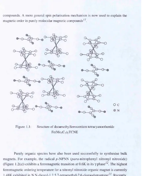
compounds. A more general spin polarisation mechanism is now used to explain the magnetic order in purely molecular magnetic compounds^

O '

o

c

© N

Figure 1.1: Structure of decamethylferrocenium tetracyanoethenide

Fe(Me5C5)2TCNE

Purely organic species have also been used successfully to synthesise bulk magnets. For example, the radical p-NPNN (p^tra-nitrophenyl nitronyl nitroxide) (Figure 1.2(a)) exhibits a ferromagnetic transition at 0.6K in its y phase^^. The highest ferromagnetic ordering temperature for a nitronyl nitroxide organic magnet is currently 1.48K exhibited in N,N-dioxyl-1,2,5,7-tetramethyl-2,6-diazaadamantane^-^. Recently, a significant increase of ordering temperatures in purely organic radical magnets was achieved with the sulphur-nitrogen dithiadiazolyl radical /^-NC-C^F^-CNSSN* (Figure 1.2(b)) which exhibits weak ferromagnetism below Tc = 36K in its (3 phase^^.

arrangement to provide an efficient magnetic exchange pathway in at least one direction (§2.6.3).

Figure 1.2(a): Structure of the organic radical para-Nitrophenyl Nitronyl Nitroxide

{p-NPNN)

Figure 1.2(b): Structure of the organic radical p-NC-C^F^-CNSSN'

7.2.2

M olecular based magnets with extended lattices

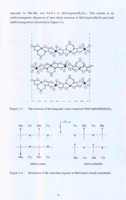
opposed to M n-M n and Cu-Cu in M nC u(pba)(H2 0 )3. This results in an antiferromagnetic alignment of inter-chain moments in M nCu(pba)(H2 0 ) 3 and bulk antiferromagnetism (illustrated in Figure 1.4).

I

o

Figure 1.3: The stmcture of ferrimagnetic chain compound MnCu(pba0 H)(H2 0)3.

Mn Cu Mn Cu

1 1

t t

Mn Cu Mn Cu

MnCu(opba)

▲ 4

T T

Cu Mn Cu Mn

... ... . . . 1

t t

1 1

t t

Mn Cu Mn Cu

MnCu(pbaOH)

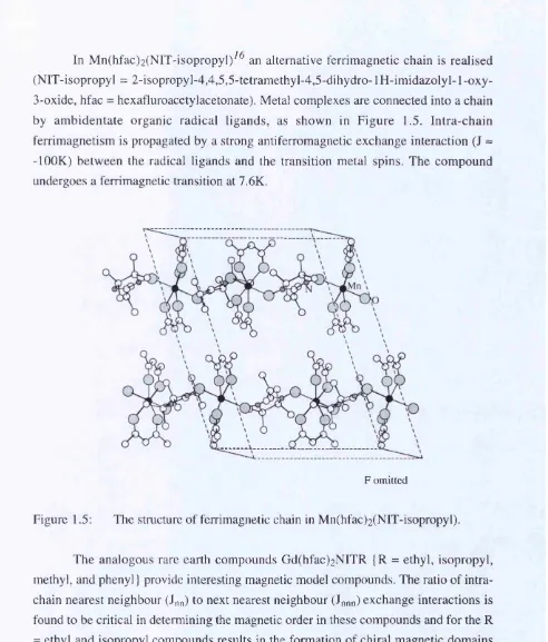
In M n(hfac)2(NIT-isopropyl)^^ an alternative ferrimagnetic chain is realised (NIT-isopropyl = 2-isopropy 1-4,4,5,5-tetramethyl-4,5-dihydro-1 H -im idazolyl-1 -oxy- 3-oxide, hfac = hexafluroacetylacetonate). Metal complexes are connected into a chain by am bidentate organic radical ligands, as shown in Figure 1.5. Intra-chain ferrimagnetism is propagated by a strong antiferromagnetic exchange interaction (J ~ -lOOK) between the radical ligands and the transition metal spins. The compound undergoes a ferrimagnetic transition at 7.6K.

F o m itte d

Figure 1.5: The structure of ferrimagnetic chain in Mn(hfac)2(NIT-isopropyl).

The analogous rare earth compounds Gd(hfac)2NITR {R = ethyl, isopropyl, methyl, and phenyl} provide interesting magnetic model compounds. The ratio of intra­ chain nearest neighbour (J n n ) to next nearest neighbour (J n n n ) exchange interactions is

found to be critical in determining the magnetic order in these compounds and for the R = ethyl and isopropyl compounds results in the formation of chiral magnetic domains and a suppression of a transition to long-range magnetic order^^.

In general, magnetic ordering temperatures in one dimensional magnetic systems are restricted to low temperatures by the limiting strength of the inter-chain exchange interactions Jintra-chain » Jinter-chain- The design of molecular based materials

prepared by this method. By choosing combinations of and [M*^i(CN)6]^' in order to maximise the antiferromagnetic/ferromagnetic interactions (see §2.4)^^"^^ between adjacent spins high magnetic ordering temperatures have been achieved; for example, C sN i* * [C r^* i(C N )6 ] (Figure 1.6) becom es ferro m ag n etic at Tc = 90K , C r”3[Cr^**(CN)6 ] 2 is ferrimagnetic Tc = 240K^^ and the room temperature magnet (V2+,v3+)n[Cr(CN)6]m.3H20 (n,m = variable) Tc= 315-340K^^

,Cs

ONi

Figure 1.6: The structure of three-dimensional lattice compound CsNiCr(CN)6.

Novel magnetic lattices have also been obtained via a molecular based approach. The com pound (r a d ) 2 M n 2 [ C u ( o p b a ) 3 ( D M S O ) ] .2 H 2 0 ^ ^ ’^-^ {rad = 2 -(l- methylpyridinium-4-yl)-4,4,5,5-tetramethylimidazoline-1 -oxy 1 3-oxide}, for example, is a unique lattice consisting of two equivalent perpendicular but interlocked honeycom b layers of connected m olecular units. The com pound undergoes a ferrimagnetic transition at 22.5K. Identical magnetic behaviour in the related simple

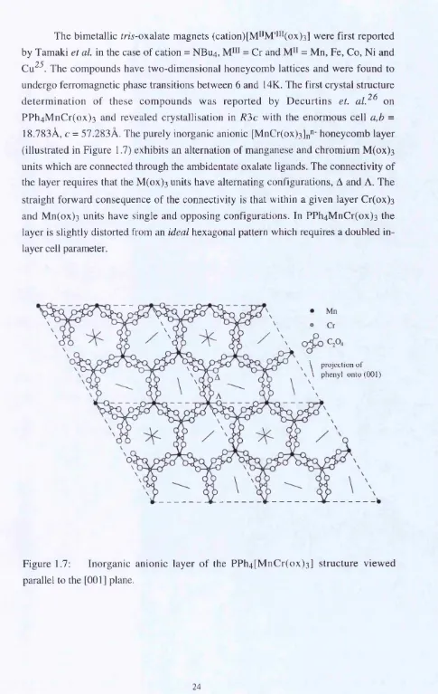
The bimetallic fm -oxalate magnets (cation)[M^*M'*i*(ox)3] were first reported by Tamaki et a l in the case of cation = NBU4, = Cr and = Mn, Fe, Co, Ni and Cu^^. The compounds have two-dimensional honeycomb lattices and were found to undergo ferromagnetic phase transitions between 6 and 14K. The first crystal structure determ ination of these com pounds was reported by D ecurtins et. a l ^ ^ on PP h4M n C r(o x) 3 and revealed crystallisation in R?>c with the enormous cell a,b = 18.783Â, c = 57.283Â. The purely inorganic anionic [MnCr(ox)3]n"‘ honeycomb layer (illustrated in Figure 1.7) exhibits an alternation of manganese and chromium M (ox) 3 units which are connected through the ambidentate oxalate ligands. The connectivity of the layer requires that the M (ox) 3 units have alternating configurations, A and A. The straight forward consequence of the connectivity is that within a given layer Cr(ox) 3 and M n(ox) 3 units have single and opposing configurations. In PPh4M nCr(ox) 3 the layer is slightly distorted from an ideal hexagonal pattern which requires a doubled in­ layer cell parameter.

^ projection o f phenyl onto (001)

Mn=A, Cr=A

Mn=A, Cr=A

M n=A, Cr=A

M n=A ,C r=A

M n=A, Cr=A

Mn=A, Cr=A

Figure 1.8: The PPh4[MnCr(ox)3] structure viewed parallel to the (100) plane (with one PPh4+ cation displayed per layer).

The R'ic structure of PPh4M nCr(ox) 3 denotes a six layer repeat, illustrated in Figure 1.8. As a consquence of the symmetry consecutive [M nCr(ox)3]n"' layers contain alternating configurations for each metal. The six layer repeat can be defined as (a-b'-c-a'-b-c'), where ' refers to a reversal of M(ox) 3 configurations in the layer.

each honeycomb layer vacancy is filled, giving four cations per layer within the unit cell. Figure 1.7 shows the axial phenyl ligand that penetrates the honeycomb layer vacancy projected onto the [001] crystal plane. One phenyl ligand is disordered by the axial three-fold symmetry and lies in the non-distorted honeycomb site of the layer. The cation positions illustrated in Figure 1.8 exemplify the rhombohedral centering of the cell which generates layers 0, 2 and 4 and the layers 1 ,3 ,5 generated by the glide plane symmetry.

The compound NBu^MnCr(ox) 3 was also found to crystallise in R3c with the reduced cell a,b = 9.414Â c = 53.66Â. The non-distorted hexagonal honeycom b inorganic layer of this compound is shown in Figure 1.9. The cell requires only one symmetry independent oxalate group. The tetrabutylammonium site is similar to that of the tetraphenylphosphonium cation in PPh4MnCr(ox) 3 with one, approximately axial, butyl ligand axially penetrating the layer vacancy; however, in the structure the butyl groups are highly disordered and not exactly determined^

Figure 1.9: Inorganic zero layer of the NBu4[MnCr(ox)3] structure viewed parallel to the [001] plane

* th e a u th o r w ish e s to th a n k P ro fe s s o r L .O . A to v y m a n n an d D r. G .V . S h ilo v fo r th e ir k in d p ro v is io n

An alternative lattice built from connected rm-oxalate units was originally identified by Tamaki et al? ^ In contrast to the honeycomb layers, consisting of alternating A and A

M (o x)3 configurations, this structure contains only one configuration A or A within the

lattice. The connecting units now generate chiral helical nets in three dimensions. This lattice type has been realised in a number of different metal oxalate based magnetic m aterials; for exam ple, {[Fe^^(bipy)3]2+[Fe^i2(o x )3]2-}n^*^’'^^ which becom es antiferromagnetic at around 15K. Figure 1.10 shows the oxalate backbone of this lattice. {[Fe‘^(bipy)3]2+[Fei*2(ox)3]2-}n is cubic [a,b,c = 15.42Â} and crystallises in the chiral space groups F4332 or F4i32 depending on which M (ox) 3 configuration is contained within the lattice (A = M 3 3 2 and A = P4i32).

It is interesting to note that a chiral oxalate crystal is formed with the molecular cation [Fe^i(bipy)3]^+ which has the chiral point group D3 and that crystallisation from racem ic m ixtures of [M(ox)3]3- and [F e"(b ipy )3]^+ results in resolution o f both components within the crystals: A-[Fe*^(bipy)3]^+ enantiomers always crystallise with the A-M(ox) 3 units and vice versa (A-A).

It can be concluded that the cation used in the synthesis of metal fm -o x alate magnets acts as a template to both two-dimensional and three-dimensional lattices depending upon its shape, charge and symmetry.

1.3 Scope of the research

The work reported in this thesis is concerned with the two-dimensional metal

diffraction data o f the equivalent cation compounds (cation)M^^Fe(ox) 3 in §4.2. Chapter 4 also includes an investigation of the magnetic order in compounds PPh4(- d2o)MnFe(ox) 3 and PPh4(-d2o)FeFe(ox) 3 by powder neutron diffraction.

Chapter 5 details a thorough investigation of the magnetisation behaviour of the compounds (cation)MHFe(ox)3, particularly the (cation)FeFe(ox) 3 series, with SQUID AC and DC magnetom etry techniques. Chapter 6 contains results o f physical experiments carried out on the (cation)FeFe(ox) 3 compounds using the local magnetic probe methods; Mossbauer spectroscopy (experiments not performed by the author) and M uSR spectroscopy experiments performed on the EMU instrument at the ISIS pulsed muon facility.

CHAPTER 2

Magnetic theory

'Few subjects are more difficult to understand than magnetism ’ Encyclopaedia Britannica, Fifteenth Edition 1989.

Despite the above, it is the purpose of this chapter to develop some theories of magnetism. The compounds examined in this thesis are two-dimensional insulating magnets and hence discussion focuses on superexchange effects between localised spins in layer lattices. Particular attention is given to ferrim agnetism and antiferromagnetism. Molecular field theory (§2.6) is developed to illustrate the variety of magnetic order in ferrimagnets (the Neel order types); however, the quantitative inaccuracies inherent in the approximation, especially with regard to low dimensional magnets, are noted.

2.1 Susceptibility

The electronic energies of all compounds are perturbed by a magnetic field and they acquire a m agnetisation. The response of the m agnetisation M to a field H is characterised by a magnetic susceptibility %.

% = B M /8H (2.1)

The susceptibility behaviour of a compound denotes its magnetic classification. Diamagnetic materials, for example, expel lines of magnetic flux and have negative susceptibilities (% <0). Diamagnetism arises from the interaction of a field with paired electrons and hence is present in all compounds. The susceptibility of a compound is usually corrected for its intrinsic diamagnetism ( -1 0'^ emu mol'O by subtraction of its estimated value using the additive Pascal constants^.

param agnetic spins follow s a B rillouin function^'^ which in low fields gives susceptibility that follows the Curie Law of paramagnetism, Equation 2.2; where C is the Curie constant and is calculated as Ng2|iBV(7+l)/3k.

X = C / T (2.2)

Param agnetic ions with therm ally populated electronic states require a perturbation approach, used by Van Vleck"^^, to derive their susceptibilities.

2.2 Magnetic interactions

In insulating solids, localised spins can interact by number of different mechanisms. The dominant interaction is usually magnetic superexchange which is covalent in origin. Isotropic (Heisenberg) superexchange in a dimer with spins Sa and Sb can be described by a Hamiltonian of type (2.3), where J is the exchange strength. Clearly, J = +ve favours ferromagnetic alignment and J = -ve an antiferromagnetic alignment of spins.

H = - 2 J S ^ S ^ (2.3) A theoretical calculation of J has been attempted by Anderson^^; however, qualitative interpretation is achieved via the Goodenough-Kanomori rules^^”^^. To summarise, (i) magnetic orbitals with a large overlap have antiferromagnetic exchange; (ii) magnetic orbitals with an expected overlap due to proxim ity, but are non­ overlapping (e.g. orthogonal orbitals) have ferromagnetic exchange and (iii) magnetic orbitals that overlap with empty orbitals give ferromagnetic exchange.

U npaired magnetic spins also interact through their dipoles, according to Equation 2.4; where and jUg are the magnetic moments of each spin and r^B is the vector distance between the two atoms a and B. The dipolar interactions in first row transition metals are weak in comparison to magnetic superexchange effects and, hence, play a secondary role in the magnetic order.

2.3 Long-range magnetic order

Magnetic superexchange interactions between spins in an extended lattice can result in a phase transition to long-range order at a critical temperature Tc. This can be followed by su scep tib ility , specific heat and neutron diffraction experim ents (§3.1.2). Ferromagnetic transitions are characterised by local moments aligning spontaneously in the same direction within the lattice. Antiferromagnetic transitions occur when moments align in antiparallel directions, leading to zero spontaneous m agnetisation. A ferrim agnetic state results when spins align antiferrom agnetically but with non­ compensating local moments. A further case of weak ferromagnetism or 'spin-canting' (§2.3.3) can occur in antiferromagnetic systems when ordered spins are canted at a small angle from exact antiparallel alignment, resulting in a non-zero spontaneous magnetisation in the direction of canting.

2 .3.1 M agnetic m odel Hamiltonians

A system o f interacting classical spins can be defined with respect to its spin dim ensionality (n) and exchange dim ensionality, (J^^J^Jz)- The general case is described by the magnetic model Hamiltonian (2.5). Specifically; = J), = and n = 3 is known as the Heisenberg model; 0, = 0 and n = 2 categorises the Planar model; whilst = Jy = 0, 0 and n = 1 corresponds to the Ising model.

= (2.5)

i< j

In the transition metal series superexchange interactions are usually isotropic. However, collective anisotropy arises from single ion anisotropy terms which manifest through spin-orbit coupling and crystal field effects; e.g. (h.s.)Fe^* ions typically show Ising behaviour. The anisotropy of the system may best be described by a second term in the model Hamiltonian as in (2.5), where D describes the anisotropy in a uniaxial system. If D-» +oo moments lie along the z-axis whilst for D-^-oo they are constrained to the plane.

hence do not exhibit transitions to long-range order. Two-dimensional systems are on the border of order and disorder with only the Ising 2-D model exhibiting a transition to long-range order. The two-dim ensional XY model (Jjc = Jy 0, = 0 and n = 3) exhibits a transition to a state with infinite susceptibility but without a spontaneous magnetisation.

Table 2.1: Spin and lattice dimensionalities exhibiting a transition to long-range magnetic order T > OK.

d = 1 d = 2 d = 3

Ising no yes yes

XY no > oo yes

Heisenberg no no yes

Real layer lattice magnets are best described as quasi two-dimensional spin systems because weak inter-layer exchange interactions J', such that J' « J, act to couple the layers. A transition to long-range magnetic order in any qu a si two- dimensional lattice will occur when two-dimensional spin correlations (characterised by a correlation length become large enough that the inter-layer coupling, which scales as can overcome thermal effects.

The anisotropy in real crystals is often only an approximation of the model Hamiltonians (discussed above). For example, finite D = +ve and D = -ve values in (2.5) describe respectively Ising and Planar type anisotropies to Heisenberg spins. A finite Ising type anisotropy in a quasi two-dimensional magnet will cause a transition to long-range magnetic order when anisotropic energy overcomes the thermal energy. This is classified as an anisotropy crossover. Indepth discussion of critical phenomena in two-dimensional magnets e.g. lattice and anisotropy crossovers is beyond the scope of this thesis. For more information see for example [De Jongh L. J.; 1990]^^.

2 .3 .2 M olecu lar f ie ld theory

M olecular field theory or Weiss mean field theory is a powerful approximation to exchange Hamiltonians of type (2.5). In essence the sum of the exchange terms acting on a single spin site are approximated to a mean exchange field, which acts to orient spins below the bulk ordering temperature T^. Considering only the z-spin components of a ferromagnet in an axial field H, the Hamiltonian (2.6)

H = - 2 X ■ Si -g /ie H • 'Z S , (2.6)

becomes for each spin Sj,

H».P = - \ 2 Z J { S ‘) + g^LBmS] (2.7)

Where is the mean z-spin component of all spins interacting with Sj. The single ion Hamiltonian (Equation 2.7) is that of a paramagnetic spin perturbed by an effective field Heff = H + Hm. f which simplifed to include only nearest neighbour ( z ) terms becomes,

Hmf = /giXB = 2zj(& ')/g/tB = AM, (2.8)

The Weiss molecular field constant A = 2zJ / relates the molecular field to the spontaneously induced magnetisation, M*, observed in ferromagnets below Tc. Hence, the spontaneous magnetisation is exactly that induced in a param agnet by an external field equal to the molecular field Hm.f. (i.e. the m agnetisation follows a Brillouin function).

sublattice A, to a first approximation, is that from exchange effects with the B magnetic sublattice and vice-versa (Equation 2.9).

“ ^ext

H r - + ^ B A ^ A

(2.9)

Extending the two sublattice model to the case where the spins on each sublattice are uncompensating, Neel postulated the ferrim agnetic ground state in 1 9 4 8^^. N eel's model case was based on the general spinel A[B] 2 0 4 lattice containing (for simplicity) only one magnetic ion distributed between the two magnetic sublattices. In zero external field the internal fields (now in Neel notation) are.

= n{aXM ^ + £}aM ^)

(2.10)

Hg = + eXM^)

W here

X

and fJLare the fractional occupancies of the magnetic ion in the A and B sublattice sites respectively

( X + f i

= 1); a and p represent the Weiss field ratios A,aa/^ab and Abb/Aba (Aab = A ra ), n is the proportionality constant 1 /A a r , /^ a and M r are the magnetisations of the A and B sublattices when fully occupied, whilst e = +/-1 (= -1 for ferrimagnetism and antiferromagnetism). Solving for a minimum in molecular field energy (Equation 2.11) at absolute zero gives four possible solutions for the saturated spontaneous magnetisation Ms = IMa - M^\ = IAMa + £/xMr| (see Table 2.2). A further consideration of both the variation in magnetisation near Tc (by expansion o f the Brillouin function) and around absolute zero gives in total six possible ferrimagnetic ordering types (M, N, P, Q, R and V). The forms o f the magnetisation curves are illustrated in Figure 2.1. The variation of a and P i.e. the relative inter and intra sublattice exchange coupling determines the ordering type. The Neel plot (a,p) for the case

X / f i

= 2/3 is illustrated in Figure 2.2.

Type M M, Type V

comp

Ms _{Type R}

Type P Type N

comp

2

-1

-A

-2

-Figure 2.2: The (a,P) Neel plot for ÀJfi=2l3

Table 2.2: Magnetic characteristics of the Neel ferrimagnetic ground states

Plot region Solution

^

Mb

M

Neel type

GASB

I

paramagnetism G

ACF

IV

-fj/a ju //(1- 1/d) M

FCE

II

A

f i

//—

A

P,Q,N

ECSH

m

A

//

A (l+1//^

R,V

The temperature evolution of magnetisation in Neel types M, R and V have a finite slope at T = OK (3M/3T ^ 0) which violates the third law of thermodynamics and hence they are not realised in experimental ferrimagnets.

The Neel types N, P and Q have many experimental examples. Type Q has a conventional magnetisation curve following a Brillouin function below Tq. Type N exhibits a temperature of compensation (Tcomp) where the m agnetisation on each sublattice is equal and opposite and hence ( T= Tcomp) = IM^- Mgl = 0. Figure 2.3 illustrates the relative temperature dependence of each sublattice magnetisation that will give rise to a type N magnetic order.

comp

Figure 2.3: Showing the relative magnetic sublattice ordering for Neel type N ferrimagnetic order

-to Ms = Ma - Mb above Tcomp- It is a feature of molecular field theory that the exact form of the type N magnetisation curve can not be determined.

The high temperature susceptibility behaviour of magnets may be shown via

molecular field theory to follow the Curie-Weiss law (Equation 2.12).

Generally, the Curie-Weiss law is used as an interpretation of the magnetic interactions in a spin system above Tc; where 0 = +ve indicates ferromagnetic interactions and 0 = -ve antiferromagnetic interactions. Molecular field theory predicts that ITc/0| = 1 for ferromagnets, antiferromagnets and ferrimagnets. Hence, the measured experimental deviation of ITc/0| from unity in a magnet is a measure of its deviation from molecular field theory.

It can easily be shown that, in a system with z nearest neighbours with exchange coupling strength J, the Weiss constant and hence Tc are given by (2.13).

0 = Tc = 2/(7+l)zJ/3k (2.13)

The quantative inaccuracy of molecular field theory is particulary apparent for low dimensional magnets. For example, the assumption of uniform exchange clearly breaks down in two-dimensional systems. Short-range magnetic order effects above Tc are critical in determining their behaviour and are not accounted for within molecular field theory.

2 .3 .3 Spin canting

W eak ferromagnetism or 'spin-canting' occurs when antiferromagnetic spins align in non exactly antiparallel, directions to one another. In a two-sublattice antiferromagnet, canting results in a small ferromagnetic moment measurable in the direction of canting below Tc. The canting can originate from a variety of effects e.g. spin-orbit coupling, dipolar interactions or single ion anisotropy.

An antisymmetric Dzyaloshinkii-Moriya exchange Hamiltonian"^^ (Equation 2.14) may be used to describe some interactions that lead to canting. W here the vector

CHAPTER 3

Experimental techniques

3.1 Diffraction

A crystal structure is composed of both a lattice, an infinite array o f lattice points generated by the primitive vectors a, b and c according to Equation 3.1, and a basis, a chemical array located on each lattice point, such that (3.1) has translational invariance. A unit cell of a crystal structure is a convenient volume used to generate the structure purely by translational symmetry. The primitive unit cell contains only one lattice point and hence its translational symmetry is exactly that of (3.1).

= n if l + n 2 ^ + n s c ( 3 . 1 )

{nj = any integer}

Bravais lattices are the fourteen distinct crystal lattices which are derived from the seven crystal systems available to lattice arrays.

The reciprocal lattice is a useful concept in diffraction theory. Each lattice

(a,b,c) has an associated reciprocal with vectors (a*,b*,c*) related to the direct lattice

by Equation 3.2.

v = (3.2)

a { b x c ) a { b x c ) a - i b x c )

(a* • a = b* ' b = c* ■ c = \, a* b = a* - b = a* - c = etc = 0)

As a consequence of the reciprocal lattice definition, every set of M iller (h,k,l) planes within the direct lattice corresponds to a perpendicular reciprocal lattice vector T, as in Equation 3.3. The modulus of a reciprocal lattice vector (ItI) is in fact the reciprocal of the shortest distance between the associated Miller planes (dhki), l%1=

Elastic scattering of X-rays or neutrons in crystals results from constructive interference or Bragg reflection from the set of lattice planes (h,k,l) at a direction where there is zero phase change between beams reflected from adjacent planes. This can be expressed qualitatively as Bragg's law and geometrically, in reciprocal space, by means of the Ewald construction (Figure 3.1). Bragg reflection is therefore expected when the Ewald sphere crosses a reciprocal lattice point P associated with the direct planes (h,k,l) parallel to IP at sinGy = \€k!2, i.e. at the Bragg angle.

nA.=2dhkisin0b (3.4)

D iffra c te d b e a m

In c id e n t b e a m

Figure 3.1: The Ewald construction as a condition of elastic diffraction

length in neutron diffraction (more commonly referred to as bj). refer to the partial coordinates of the atoms within the cell. Wi are D ebye-W aller isotropic tem perature factors which result in a reduction in scattered intensity from thermal motions.

Fhk] = Zf,exp(-2m (h% . + ky. -H lz.)ex p (-W ,) (3.5)

i

In some cases systematic absences occur (Fhki = 0) where the lattice planes of a crystal are arranged so that reflection from them results in a total destructive interference of the diffracted beam.

3.1.1. P o w d er X -R ay D iffraction

In X-ray diffraction elastic scattering results from the coherent emission of X-rays from electrons accelerated by the incident X-ray beam. The atomic structure factor f; is therefore a summation over all the electrons in an atom. This results in a monotonie increase in the structure factor with atomic number and a fall-off of scattering with (sinG)/^, the X-ray form factor.

In this thesis powder X-ray profiles were collected on a Siemens D500 diffractom eter, set in Bragg-Brentano reflection geometry, using C u K a doublets {CuKtti = 1.54051Â, C u K a2 = 1.54433Â} with a K ra tio { K a i/K a2} of 0.5. The X- ray beam slits were kept constant at 0.3m m for all experim ents. D uring the experim entation period the X-ray source was replaced a number of times. Samples were mounted on a flat plate ceramic, such that the full beam area 3x15mm^ was directed at the sample. Profiles were recorded as step scans at intervals of 0.02 in two- theta. Initial characterisation scans were carried out with a total collection time o f 45 minutes, corresponding to a count time of one second. Profiles presented in Chapter 4 are from long scans with a count time of 1 0 seconds giving a total collection time of around 1 2 hours (generally performed overnight).

3.1.2. N eutron diffraction

Also the nucleus behaves effectively as a point scatterer to incident neutrons and hence does not incur a form factor effect.

Neutrons are spin-1/2 particles and interactions between the neutron's magnetic moment and unpaired spins on atoms results in elastic magnetic scattering. Coherent magnetic diffraction (magnetic Bragg reflection) will occur if there is long-range magnetic order between scattering spins. In magnetically ordered materials neutron diffraction structure factors, must therefore be described as a sum of contributions from nuclear and magnetic scattering. In an unpolarised neutron diffraction experiment the diffraction intensities (Ihki) simplify to the sum of the squared moduli of the two terms (Equation 3.6).

Ihki = IFhkf = IFNhkll^ + IPMbkll^ (3.6)

The magnetic structure factor pMhki^^ is given in Equation 3.7. The term pi is the magnetic counterpart to the nuclear scattering length equal to (e^2m c^)g7f(T), with y the neutron magnetic moment and gJ the effective magnetic moment of the scattering atom. The magnetic form factor f(r) arises as a result of the atomic moment's spatial distribution.

pMhki ^ Z 9,P,Gxp(-2m(h%,. -h ky,. 4- lz,)ex p (-W ,) (3.7)

The magnetic structure factor is dependent upon the spin orientations within the unit cell. It is therefore a vector quantity and this is reflected in the magnetic interaction vectors q\ within the structure factor summation. The general magnetic interaction vector q is defined as in Equation 3.8, where the scattering vector T is the unit reciprocal lattice vector perpendicular to the scattering planes and M is a unit vector parallel to the spin direction.

q = T ( T - M ) - M (3.8)

This is shown graphically in Figure 3.2. q'^ can be simply related to the angle between the scattering and spin vectors, Tj, as

In a diffraction experiment domain effects within an ordered magnetic material can cause a variety of q\ for each spin and the measured diffraction intensity is then proportional to the average <q?>.

S c a tte rin g p la n e

I n c id e n t n e u tro n b e a m

S c a tte re d n e u tro n b e a m M a g n e tis a tio n v e c to r

S c a tte rin g v e c to r

Figure 3.2: The geometry of magnetic Bragg reflection

The description of a magnetic unit cell requires information on spin directions and the configurational symmetry between them. It is often the case that the magnetic symmetry is not the same as the nuclear symmetry. Indeed in the case of a second order phase transition^^, we expect 'broken sym m etry' with the appearance of the order parameter and therefore the magnetic group to be a subgroup of the nuclear group. The m agnetic cell may also be altered with respect its nuclear counterpart. It can be described with respect to a probagation vector K, Equation 3.10, which relates the moment at the direct lattice origin Mq to the moment Mn at the lattice point

M„ = Mq exp(2mf^ • k) (3.10) Here K= (0,0,0) describes an unaltered cell whilst k = (1/2,0,0) corresponds to a magnetic cell that is doubled along the a- axis with respect to the nuclear cell.

through a mirror plane; (iii) spin components perpendicular to a mirror plane are invariant, and inverted through a two-fold axis. In the magnetic space group definition, anti-symmetry operations are further defined when the spin character change is opposite to that expected from the operation. In total, 1651 Shubnikov groups are generated.

Alternatively, Bertaut'^^ used group representation analysis to identify possible spin structures, which have to be linear combinations of irreducible representations of the group. This approach has met with success in interpreting magnetic structures which can not be described by the Shubnikov groups. Indeed the Shubnikov magnetic space groups are only one dimensional representations of the group.

Reflection m Translation t Rotation 2 Inversion I

Figure 3.3: operations

Schematic representation of the behaviour of spins upon symmetry

3.1.3 P o w d er Neutron D iffraction Instruments

There are two common sources of neutrons used in neutron diffraction experiments: reactor sources and spallation sources. The powder neutron diffraction experiments reported in this thesis were performed at the Institut Laue Langevin (ILL) Grenoble, a reactor source^^. Neutrons are produced constantly in the reactor with a Maxwellian spread of wavelengths centred around the thermal energy of the modulating graphite rods and coolant D2O. Diffraction is performed at constant wavelength and a typical neutron powder diffractometer set-up'^'^ is that of Figure 3.4. Generally the neutrons are guided by collimators, controlling the beam divergence and monochromation is by a single crystal set at Bragg scattering angle for a particular wavelength, known as the take-off angle 20m.

1st c o llim a to r

M o n o c h ro m a to r S o u rc e

2n d c o llim a to r

S a m p le

3rd c o llim a to r

D e te c to r

(i) D I B instrument

The D IB diffractometer is a high intensity, medium resolution, powder diffractometer located in the guide hall at the I L L. The wavelength is fixed at 2.52Â, by a graphite focusing monochromator. High count rates are achieved with a fixed position sensitive detector (PSD), with 400 cells, covering a angular two-theta range of 80 degrees (see Figure 3.5). The data are collected in steps of 0.2 degrees, as defined by the distance between adjacent detector cells in the PSD bank.

K t *

----I Monochrom ator [

I Shutter

I Graphite filter

Neutron Beam

1

i

I Monitor I

i M ^ IShieldingl

_{[Beam S t ^}

|MuItidetectOT|

Figure 3.5: The DIB constant wavelength diffractometer

(ii) D IA instrument

via rotation of the detector bank. Monochromation is via 30 oriented Ge single crystals. A variety of wavelengths are available via rotation of the monochromator to a selected Bragg reflection plane. In the reported experiments the maximum wavelength of 2.9811Â has been used corresponding to the G e[l 13] reflection. A special graphitic filter was inserted between the monochromator and the sample, which significantly reduced higher order wavelength contaminations (k/3 < 0.1 %).

New 25-collim ator detector bank on diffractometer DIA

Reactor 60m Monochromator

Sample

650 mm

Figure 3.6: The D 1A constant wavelength diffractometer

(iii) D2B instrument

resolution and high intensity^^. The focusing converges the beam to 40cm high at the sample position, some 3 meters from the monochromator. The multi-detector bank of 64 detectors covers a solid angle in two-theta of 160 degrees. Collection is by step scans of 0.05®. The new option of a graphitic filter similar to that of D1A allowed collection at the relatively high wavelength of 2.398Â (Ge[331]) without significant contamination from higher order wavelengths. During the measurements made in this thesis the instrument was set in its high intensity mode.

020

053

a : 1 3 5 ”

b :1 6 0 "

c :1 6 5 !

d - 1 6 0 ”

e ;- l 2 0 0

f : - 2 0 0

c ir c u la r c o u n t e r s u p p o r t t r a c k ( 3 2 5 ” +)

B ^C /epoxy shielding ( 0 1 A m odel)

2 c o u n t e r b a s e

m o v a b l e b e a m —s t o p

.6 4 s o lle r c o l l i m a t o r s 5 ’ - 0 3

6 4 d e t e c t o r s H e 3 5 a t m a l t e r n a t i v e m o v a b l e b e a m - s t o p

Figure 3.7: The D2B constant wavelength diffractometer

3 .1 .4 Fitting p o w d e r diffraction profiles

In a powder diffraction experiment, with a random orientation of crystallites, lattice planes give Deybe-Scherer cones of scattering at directions determined by the Bragg condition. Equation 3.4. The three dimensional reciprocal lattice is projected onto one dim ension, resulting in overlapping scattering from planes with sim ilar dhki separations. The successful interpretation of a powder diffraction pattern relies on accurately measuring positions and intensities from a maximum number of reflections.

positions with the linear squares refinement program REFCEL^^. It was not feasible to use integrated intensities from partial pattern decomposition to solve structures, in this case, as the number of reflections that could be assigned was limited.

The Rietveld method of structural refinement^^'^^ avoids the a priori attribution of intensities to reflections and attempts to fit the entire powder profile. In the Rietveld method the residual function Sy between observed and calculated patterns. Equation 3.11, is minimised by non-linear least squares methods. W here the summation Syis over all observed points "i" in the profile with yi(obs) and yi(caic) the observed and calculated intensities of the profile at each point. The weighting function Wi is equal to

l/yi(obs)'

Sy = S '^ i(yi(.b »-yi(cic))' (3 11)

i

The intensities Yi(caic) are calculated

as;-yi(cajc) ~ A jQ (2 0 j — )Pf,ijT 4 -y,jj ( 3 .1 2 )

hkl

where s is the scale factor, L^ki is the Lorentz correction (inclusive of polarisation and multiplicity factors). Ai is the asymmetry parameter, Q is the peak shape function, Phki is the preferred orientation function, T is due to absorption and yti is the background contribution.

Peak shapes are a result of convolution of sample and instrument effects. The most simple peak shape function is a Gaussian with a Full W idth at H alf M aximum (FWHM), defined by the model parameters u, v and w. Equation 3.13.

(FWHM)^ = Mtan^ 0-1-v ta n 0 + w (3.13)

Often, as a result either of sample or instrument effects, peaks have a Lorentzian component to their shape. In this case the pseudo-Voigt function, a linear combination of Lorentzian and Gaussian functions (Equation 3.14) is often a good description of the peak shape, where T| defines the fractional Lorentzian contribution;

Asymmetric peak shapes can arise from an num ber of other effects, m ost commonly being the result of diffraction geometry. This is caused by the cutting of the curved Debye-Scherer scattering cone with a finite width detector. The asymmetric contribution A, is modelled below a certain limiting Bragg angle, where asymmetry becom es noticeable. The expression for asymmetry Aj used in the FU LLPRO F program is that introduced by Berar and Baldinozzi with four angle dependant refinable parameters'^^.

Preferred orientation effects occur when powder crystallites align preferentially with respect to their crystal habit. In planar structures preferential alignm ent of crystallites is along their [001] planes, especially in flat plate geometry, which results in increasing relative intensity from [001] reflections, to the detriment of those from [hkO]. The preferred orientation function Phki can be modelled by a number of expressions within the Rietveld approach'^^, however, the addition of such arbitrary parameters hinders successful refinement.

M inimisation of the residual Sy does not necessarily indicate a successful structural solution and there are a number of factors which characterise refinement results: the structural factor Rf, Bragg Factor Rg, Pattern factor Rp, W eighted pattern factors Rwp and the 'goodness' of fit are all defined in Appendix 1. Successful Rietveld refinement depends on, i) a good starting model for the structure; ii) an adequate description of the peak shape and its two-theta dependence and iii) sufficient information in the diffraction profile to support the structural solution. In cases where i) ii) and iii) are not all met, Rietveld refinement must be used with extreme caution.

For a variety of reasons full structural refinement from the powder diffraction data in this thesis was not possible. In particular the peaks exhibited tw o-theta dependent broadening and asymmetry characteristics that could not be modelled using the Rietveld program FULLPROF^^. However, the program's functionality has been used extensively to fit profiles to starting structural models and including features such as peak asymmetry and preferred orientation effects in refinement, so that structural information could be inferred from the powder profiles.