University of South Carolina
Scholar Commons
Theses and Dissertations
1-1-2013
An Effective Field Theory Calculation of n(p, d)γ
Cross-section for Big Bang Nucleo-synthesis
Rasha Adnan Kamand
University of South CarolinaFollow this and additional works at:https://scholarcommons.sc.edu/etd Part of thePhysics Commons
This Open Access Thesis is brought to you by Scholar Commons. It has been accepted for inclusion in Theses and Dissertations by an authorized administrator of Scholar Commons. For more information, please contactdillarda@mailbox.sc.edu.
Recommended Citation
An Effective Field Theory Calculation of n(p, d)γ Cross-section for Big Bang Nucleo-synthesis
by
Rasha Adnan Kamand
Bachelor of Science - Physics
American University of Beirut, Lebanon 2008
Submitted in Partial Fulfillment of the Requirements for the Degree of Master of Science in
Physics
College of Arts and Sciences University of South Carolina
2013 Accepted by:
Matthias R. Schindler, Director of Thesis Kuniharu Kubodera, Reader
c
Abstract
Studying the nuclear reactionn(p, d)γ and calculating its cross-section is not only a matter of interest from theoretical particle physics point of view but also from the viewpoint of cosmology. We now know that the universe is made up of only ≈ 5 % baryonic matter. So, computing the density of baryons is of particular importance to physicists in general and cosmologists in particular. Deuterium production during Big Bang Nucleo-synthesis (BBN) is very sensitive to the density of baryons, thus baryon density can be inferred from the abundance of deuterium. In order to calcu-late deuterium abundance one needs to use the cross-section of np→ dγ reaction as one of the inputs. Hence, the importance of this cross-section calculation.
In this document, a leading-order (LO) calculation of n(p, d)γ cross-section is presented using the framework of pion-less effective field theory with dibaryon fields. The computation yielded a numerical value ofσLO = 494 mb which is then compared
Table of Contents
Abstract . . . iii
List of Figures . . . v
Chapter 1 Introduction/Motivation . . . 1
Chapter 2 Nucleo-synthesis in the Early Universe . . . 3
2.1 The Early Universe . . . 3
2.2 Big Bang Nucleo-synthesis . . . 7
Chapter 3 Effective Field Theory (EFT) . . . 11
3.1 Effective Field Theory Techniques . . . 13
3.2 Pion-less EFT with Dibaryon Fields . . . 15
Chapter 4 LO np−→dγ cross-section in dEFT(/π) . . . 24
4.1 LO calculation of the amplitudeY . . . 26
4.2 From amplitude to cross-section . . . 32
Chapter 5 Conclusion . . . 36
List of Figures
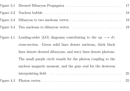
Figure 3.1 Dressed Dibaryon Propagator . . . 17
Figure 3.2 Nucleon bubble . . . 18
Figure 3.3 Dibaryon to two nucleons vertex . . . 19
Figure 3.4 Two nucleons to dibaryon vertex . . . 19
Figure 4.1 Leading-order (LO) diagrams contributing to the np −→ dγ cross-section. Green solid lines denote nucleons, thick black lines denote dressed dibaryons, and wavy lines denote photons. The small purple circle stands for the photon coupling to the nucleon magnetic moment, and the gray oval for the deuteron interpolating field. . . 25
Chapter 1
Introduction/Motivation
The early universe was a nuclear reactor. A few minutes after the Big Bang, a series of reactions took place whereby the first light nuclei were formed. These are Deu-terium (D), Tritium (3H), Helium 3 (3He), Helium 4 (4He) and Lithium 7 (7Li). The process of formation of the above nuclei is known as the Big Bang Nucleo-synthesis (BBN) which started when the universe was approximately 3 minutes old and lasted for about half an hour after the Big Bang. The first step in nucleo-synthesis is the binding of a proton p and a neutron n to build a deuteron d(the nucleus of a Deu-terium atom) through the following reaction n+p → d+γ, where γ denotes a photon.
done where the cross-section was evaluated to higher orders using again pion-less EFT [1, 2, 3]. Moreover, the polarized np reaction ~n+~p → d+γ has been studied within the framework of EFT to calculate some spin-dependent observables [4]. We will talk about this in a little bit more detail in the last chapter.
Chapter 2
Nucleo-synthesis in the Early Universe
The first few elements in the periodic table were synthesized approximately three minutes after the birth of the universe at the time when the temperature was low enough to allow the formation of light nuclei through the process of nucleo-synthesis. In the course of this chapter, we will review in section one the history and stages of the universe after the “big bang” took place up until the stage of BBN, which will be discussed in the second section.
2.1
The Early Universe
How did the universe come into existence? Well, there is no one final and conclusive answer that explains the birth of our universe. A few theories have been proposed to unravel the mystery of the origin of the cosmos. The Big Bang model is the most widely accepted cosmological theory of the early universe and its development after the moment of the “big bang”. It was put in proposition as the “hypothesis of the primeval atom” in 1931 by Georges Lemaitre [5], a Belgian priest and physicist, and later supported and developed by Gamow [6].
at the Planck scale which is around 1.22×10¹⁹ GeV. So we will not discuss what hap-pened during the Planck era and shortly after that, but our discussion of the history of the universe will start after the so called “inflationary epoch” when the early uni-verse is permeated with a plasma of elementary particles, namely quarks, leptons and their anti-particles and of course photons.
2.1.1 Evolution of the early universe after the quark epoch
About 10−6s after the “big bang”, the temperature dropped down to the point
where the average interaction energy between quarks fell below the binding energy of hadrons inside which the quarks got confined. Before the formation of hadrons, it is theorized that the universe was filled with quark-gluon plasma as the temper-ature was too high for stable hadrons to form. The conditions that give rise to a quark-gluon plasma are still unknown; however, the strong force that binds quarks into hadrons is known to become weaker at very high temperatures, a property called “asymptotic freedom”.
In what follows, I will base my description of the stages of cosmic evolution mostly on Steven Weinberg’s The First Three Minutes [7].
At t≈0.01s after the “big bang”: The temperature is around 1011 K, and the
universe is in a state of thermodynamic equilibrium which means that there is no net flow of matter or energy. A system in thermodynamic equilibrium is characterized by a uniform temperature. The universe is dominated by a soup of matter that includes electrons (e−), positrons (e+), neutrinos (ν), anti-neutrinos (¯ν) and radiation
(pho-tons). The percentage of nucleons is small at this time, in the ratio of one nucleon for each 109 photons [7]. Due to the high temperature, the rate of collisions between
(n/p≈1) due to the following two reactions
p+e− ←→n+ν
and
n+e+←→p+ ¯ν
The universe continues to cool and expand.
At t≈0.12s after the “big bang”: T≈ 3×10¹⁰ K and the state of the universe
is still pretty much the same. Expansion continues and as the temperature drops further, the reaction in which neutrons turn into protons is favored because neutrons are heavier and thus easier to form lighter protons. So the (n/p) ratio is no longer equal to unity. The number of nucleons is now 38% neutrons and 62% protons.
At t≈1.10s after the “big bang”: The temperature cools down to about 1010
K. The density is decreasing as the universe is still expanding. This falling off in the energy and density increases the mean free path of neutrinos and their anti-particles, so they are almost free particles now. The neutrinos then decouple and cease to be in thermal equilibrium with the rest of the other particles. Protons and neutrons at this stage cannot combine to form the light nuclei because the temperature is still relatively high for the nucleons to be bound.
particles are annihilated fast. Stable nuclei like 4He can now be formed; however, this is not achieved during this phase. The reason behind that is the following: the production of4Hehappens gradually in a series of two-particle reactions starting with
deuteron productionn+p → d+γ, but the deuteron nucleus is loosely bound. So at the current temperature, as soon as deuteron nuclei are formed, they are quickly dissociated by the inverse reaction d+γ −→ n+p. Thus, heavier nuclei are not created.
At t≈ 3 minutes after the “big bang”: It is approximately 109 K at this period,
and our universe is mainly filled with neutrinos, their anti-particles and photons. A reaction which further decreases the number of neutrons has started to take place: the decay of free neutrons (n −→ p+e−+ ¯ν). The (n/p) ratio is now around 1:7. The universe is still hot for the “deuteron bottleneck” to be overcome, in other words, deuteron nuclei continue to be broken up once they are created.
A little later than three minutes, the temperature becomes low enough for deuteron nuclei to form and not be destroyed, so then the phase of nucleo-synthesis “officially” commences! But as I promised earlier in the “Motivation”, Big Bang Nucleo-synthesis will be discussed in a somewhat thorough manner, and the upcoming section will be devoted to that purpose.
2.1.2 Observational evidence of the Big Bang
Penzias and Wilson is a relic of the big bang. The CMB is a “leftover” radiation from the early stages of the development of the universe. The third supporting evidence is the abundance of the first light elements as predicted by BBN. The calculated abundances of the primordial elements are in close agreement with their measured values. Galactic evolution as predicted and explained by the Big Bang theory agrees with the observations of the formation and distribution of galaxies. This constitutes the fourth pillar of the Big Bang model.
2.2
Big Bang Nucleo-synthesis
Before we talk about the physics of primordial nucleo-synthesis, it would be informa-tive to mention very briefly the history of the theory of BBN.
In 1942, G. Gamow proposed that the elements that we know today had their origins during the evolution of the universe after the “big bang”. In their seminal 1948 paper entitled "The Origin of Chemical Elements", Alpher, Bethe and Gamow suggested that elements of the periodic table were formed in a series of neutron capture re-actions a few minutes after the birth of our universe [6]. However, further research showed that the big bang was responsible for the production of the first few elements only, mainly4He[8], the reason being that nuclei with mass numbers 5 and 8 are un-stable and the Coulomb repulsion dominates as the temperature drops. A few years later, two independent research papers were published explaining that the remaining elements of the periodic table (with high mass and atomic numbers) were created in stellar reactions [9, 10].
the universe [15]. BBN has been one of the pillars of the Big Bang model and a probe of not only fundamental but also new physics [16].
2.2.1 The physics processes of BBN
At T 1 MeV, thermodynamic equilibrium dominated the universe. Among other factors, the nuclear reactions which maintained thermodynamic equilibrium are
n+νe↔p+e−,
n+e+ ↔p+ ¯νe,
n↔p+e−+ ¯νe,
The neutron-to-proton ratio was fixed at (n/p) ' e−4m/T ≈ 1 where 4m = 1.293
MeV is the neutron-proton mass difference.
As the universe expanded and cooled down to around 1 MeV, the neutrinos and their anti-particles, which were kept in thermal equilibrium also via weak interaction, stopped interacting with the other particles (mainly e+ and e−). So the weak inter-actions are said to“freeze-out”, and the (n/p) ratio also froze at about (1/6). At T≈1 MeV, nucleo-synthesis kind of began with the reaction
n+p↔d+γ.
Deuteron started to form, but due to the high number density of photons (nγ) relative
to that of nucleons (nB), [η−1 = (nγ/nB) ≈ 1010], the deuteron nuclei were rapidly
photo-dissociated. Deuteron production was delayed and BBN did not kickoff until the temperature fell below the deuteron binding energy of 2.2 MeV.
half-life of t1/2 ≈ 882s. This further dropped the (n/p) fraction to approximately
(1/7) by the time of nucleo-synthesis. It is important to know that the presence of free neutrons was one of the necessary conditions for synthesizing the first few light nuclei.
When the temperature reached ≈ 0.1 MeV, the universe was a few minutes old, a little more than 3 minutes. At last, deuteron nuclei began to form via neutron capture:
n+p→d+γ,
without being dissociated, the reason being that the number of photons per baryon with energies above the deuteron binding energy was well below unity. And so the nucleo-synthesis chain started with the above reaction (deuteron production reac-tion), and the other light nuclei were formed by a series of two-body, neutron-capture reactions. Once deuteron formation took place, other nuclear reactions proceeded to produce other light nuclei mainly 4He that has a higher binding energy (E
B ∼= 28
MeV) than deuteron (Ed ∼= 2.2 MeV). Here are two possible sets of reactions
(photo-reactions) that ultimately produce Helium 4:
d+n → 3H+γ,
3
H+p→ 4He+γ,
d+p→ 3He+γ,
3He+n → 4He+γ.
Due to the instability of nuclei with mass number 5, there was another bottleneck at
4He. Among the few light nuclides produced by BBN,4Heis the most tightly bound
at mass number 5, a few reactions where the Coulomb interaction got suppressed managed to overcome the gap and form7Liand7Be. As the temperature fell below≈
Chapter 3
Effective Field Theory (EFT)
The main part of my thesis is the calculation of the n(p, d)γ cross-section which is presented in Chapter 4. The cross-section is calculated up to leading order (LO) applying the framework of pion-less EFT with dibaryon fields. Before going into the details of my calculation, I devote this chapter to introduce the general audience to EFTs. I should note that my discussion on EFTs is by no means a thorough treat-ment of this topic. I will just touch the surface trying to summarize the general idea behind EFT and explain the main points. And so the interested general reader can get more detailed and rigorous explanation/analysis in the following references [21, 22, 23, 24, 25, 26] and many others.
Let’s start our discussion by first asking the question: In Physics, what is an effec-tive theory? Well, I think that almost all physicists would agree that the theories in Physics which we know of so far are actually effective theories except a theory of
everythingwhich has not been found yet! Nature and consequently the world that
theory”. The key idea behind an effective theory is to set the parameters that are very small (negligible), in comparison to our physical quantities of interest, to zero and set those which are very large to infinity; the effects of these parameters can then be treated as small perturbations. In other words, an effective theory is valid below a certain energy scale Λ and thus in a limited energy range. It is a systematic approximation to a more “fundamental” theory which is valid at all energies including arbitrarily high energies.
3.1
Effective Field Theory Techniques
ChPT, mentioned above, is one example of an effective field theory employed in theoretical nuclear/particle physics. An EFT is a field theory framework appropriate for the description of low-energy physical phenomena. When one says low-energy, it is meant low with respect to some energy scale or energy cutoff Λ. In an EFT, only the pertinent degrees of freedom (d.o.f) are taken into account, those with mass m Λ. The heavier fields whose mass M Λ are eliminated out of the action. In constructing an EFT, theoretical physicists usually use one of the two general approaches, the bottom-up or the top-down. The top-down approach starts with the action of the high-energy theory, and the effective action is obtained by systematically integrating out the high-energy degrees of freedom. The other approach (bottom-up) constructs the effective theory action without relying on a “more fundamental” action because it is unknown. So, the effective action in the latter approach is built from scratch. In both procedures, the effective Lagrangian which describes the EFT is an expansion in terms of a sum of local operators (the sum is infinite)
Lef f =
X
i
ci Oi .
These operators Oi that are included in the effective Lagrangian must be
consis-tent with the symmetries of the high-energy theory and, as mentioned above, are constructed from the light fields. The coefficients ci are the couplings. They carry
information on the high-energy d.o.f which have been integrated out.
observ-able, we only require a certain finite accuracy of our results. This leads us to the concept of power counting. EFT corresponds to an expansion in Λq where q stands for energy, mass or momentum such that q Λ. Power counting basically helps us determine the order up to which we need to expand so as to achieve a specific accuracy (see e.g. Ref.[34]).
In field theories, while calculating observables in physical processes, one may en-counter divergent integrals. Measurable physical quantities cannot be infinite. These divergences appear as intermediate stages in field theory calculations, and they even-tually get cancelled out yielding finite values for physical quantities. So, certain tech-niques were developed in order to deal with these infinities. Treating the divergences is a two-step process starting with “regularization” and then “re-normalization”. In the first step, we “regulate” the divergent integrals, i.e. we make the apparent diver-gences look finite by introducing what is called a “regulator”. In doing so, we can then manipulate these integrals. In quantum field theory, there are a few regulariza-tion methods such as cut-off regularizaregulariza-tion, Pauli-Villars, dimensional regularizaregulariza-tion (DimReg), etc. More detailed discussion and examples can be found in [27, 28]. Later in this chapter, I will present a calculation using dimensional regularization.
the following: the divergences coming from the integrals (loop diagrams in field theo-ries) can be removed by an appropriate redefinition of the parameters (bare couplings
ci0) in the Lagrangian density.
ci0 −→ ciR = ci0 + δci(β). (3.1)
The infinities from the integrals are absorbed byδci(β). So, the parametersci0 get
“re-normalized” tociR which are finite. ciR are the observed values that get measured
in experiments.
3.2
Pion-less EFT with Dibaryon Fields
As an example of EFT, I will discuss EFT(π/) with the use of dibrayon fields. Before I go into the details of the theory, I should note that this will be a useful example in which I calculate the dressed dibaryon propagator employing dimensional regular-ization [38] and the PDS scheme [33]. The dressed dibaryon propagator will then be used in the calculations of the upcoming chapter.
Pions play an important role in mediating the nucleon-nucleon (NN) interaction; however, at low enough energies (momenta p mπ), the pions are integrated out
of the effective Lagrangian as heavy fields. So, in EFT(π/), the only relevant degrees of freedom are the nucleons. In other words, EFT(π/) is a low-energy theory suitable to describe and study reactions (at momenta p 1
R) between particles with a
When dealing with the deuteron, it was shown (see references [31, 32]) that it’s more convenient to introduce an auxiliary field called dibaryon (that can be thought of as a bound state of two nucleons), denoted byt, which simplifies computations. In Chapter 4, I will calculate the cross-section of np→dγ up to LO using EFT(π/) with the dibaryon field. The calculation involves two LO Feynman diagrams which are schematic drawings showing interaction vertices and propagators. So, to carry out the calculation, we first need to find the nucleon and dibaryon propagators and also compute the Feynman rules for the vertices. The reason why I present the dressed dibaryon propagator calculation now is that it involves a loop integral that needs to be regularized and then re-normalized, so it is a good example relevant to this chapter.
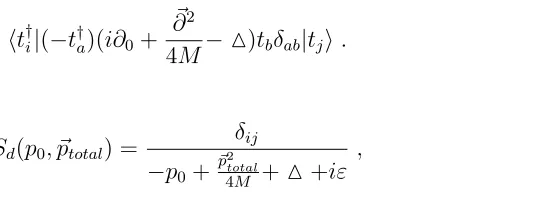
3.2.1 Dressed Dibaryon Propagator
The dibaryon propagator that enters in the cross-section calculation of the reaction
n(p, d)γis the “dressed” (full) propagator. The bare dibaryon propagator gets dressed by nucleon bubbles (loops) to all orders (see Figure 3.1). Let me denote the bare propagator bySdand the dressed propagator byD. Sdcan be derived from the kinetic
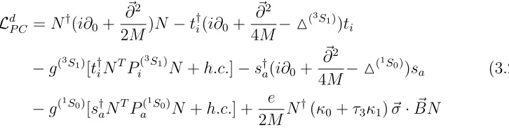
term for the dibaryon field in the Lagrangian. The Lagrangian density describing the dynamics in both the 3S1 and 1S0 channels is [32]
Ld
P C =N †
(i∂0+ ~ ∂2
2M)N −t
† i(i∂0+
~ ∂2
4M−M (3S
1))t
i
−g(3S1)[t†
iN TP(3S
1)
i N +h.c.]−s † a(i∂0+
~ ∂2
4M−M (1S
0))s
a (3.2)
−g(1S0)[s†
aN T
P(1S0)
a N +h.c.] +
e
2MN
†
(κ0+τ3κ1)~σ·BN~
= + + + ...
Figure 3.1 Dressed Dibaryon Propagator
isoscalar and isovector nucleon magnetic moments, g2 = 8π
M2r and M=
2
M r( 1
a −µ)
are the couplings with r and a denoting the effective range and scattering length, respectively, while µ is a re-normalization scale that appears later in re-normalizing the loop integral.
The dibaryon fields in the 3S
1 and 1S0 channels are represented by ti and sa,
respec-tively.
P(1S0)
a =
1
√
8τ2τaσ2, (3.3)
P(3S1)
i =
1
√
8τ2σ2σi (3.4) are the normalized projection operators where τa and σi, a, i = 1,2,3, are the Pauli
isospin and spin matrices, respectively.
As mentioned above, the bare dibaryon propagator can be derived from the dibaryon kinetic term,
ht†i|(−t†a)(i∂0+ ~ ∂2
4M−M)tbδab|tji. (3.5)
So this gives
Sd(p0, ~ptotal) =
δij
−p0 +
~ p2
total
4M +M+iε
, (3.6)
(note that the convention I am using is that in a Feynman diagram, a line stands for
i×propagator).
re-summation is explained by power counting [32]. The bare dibaryon propagator
Sd ∼ Q−2 where Q is a small momentum expansion parameter. Each vertex is
∼ Q1/2, and each loop contributes a factor of Q. So, by applying the latter power
counting scheme, every diagram in figure 3.1 counts as Q−2. Therefore, the nucleon
bubbles must be summed to all orders.
The calculation involves computing the nucleon loop integral which will be denoted by Iloop. This integral will be regularized by DimReg then re-normalized by PDS.
Although we are summing an infinite number of terms, we notice that this sum is a geometric series which has a closed form
iD=iSd(
1 1−i Iloop Sd
). (3.7)
Loop integral Iloop calculation
We first need to take a look at the loop diagram below. Let me note that we are
Figure 3.2 Nucleon bubble
working in the center of mass frame, and the incoming dibaryon has total energy E and zero momentum (E, ~0). This energy gets distributed between the two nucle-ons where one has (E2 +p0, ~p), and the other has (E2 −p0,−~p), where p0 and ~p are
loop/integration momenta. As seen in figure 3.2, there are two interaction vertices which we need to compute. The “Feynman rules” give the following vertices:
a) Incoming dibaryon to two outgoing nucleons:
−iyhNA†NB† |NR†PRSj†NS†tj |tii=−iyPi
†
Figure 3.3 Dibaryon to two nucleons vertex
b) Two incoming nucleons to outgoing dibaryon:
−iyht†i |t†jNRP j
RSNS |NANBi=−iyPABi , (3.9)
Figure 3.4 Two nucleons to dibaryon vertex
Let me note that the A, B, R, and S are spin and isospin indices carried by the nucleon fields, that is A=(a,α), B=(b,β), etc. where a,b andα,β, etc. are the isospin and spin indices, respectively. To avoid confusion, let me point out that the ‘y’ appearing in equations (3.8) and (3.9) is a general coupling that gets replaced later by the appropriate coupling constant in the different 3S1 and 1S0 channels.
Also needed is the nucleon propagator which can be derived from the nucleon kinetic term in the Lagrangian which gives
SN(k0, ~k) =
1
k0−
~k2 2M +i
We are now in good shape to calculate the loop integral. So,
Iloop = (−2iyPi
†
AB) (−iyP j AB)
Z d4p
(2π)4
i
E
2 +p0−
~ p2 2M +i
i
E
2 −p0−
~ p2 2M +i
=−2y2PABi† PBAj
Z d4p
(2π)4
1
E
2 +p0−
~ p2 2M +i
1
E
2 −p0−
~ p2 2M +i
=−2y2T r(Pi†Pj)
Z d4p
(2π)4
1
E
2 +p0−
~ p2 2M +i
1
E
2 −p0−
~ p2 2M +i
(3.11)
=−2y2(1 2δ
ij)Z d4p
(2π)4
1
E
2 +p0−
~ p2 2M +i
1
E
2 −p0−
~ p2 2M +i
=y2δij
Z d4p
(2π)4
1
E
2 +p0−
~ p2 2M +i
1
−E
2 +p0+
~ p2 2M −i
.
The factor of ‘2’ is a symmetry factor coming from the two different ways of connecting the nucleon lines to form the full loop. Note that I now used ‘p’ instead of ‘k’ for the nucleon momentum, but that doesn’t really matter since the ‘k’ that appeared in the propagator SN is just a dummy variable.
The above integral diverges linearly in 4 dimensions, so we use DimReg (see e.g. Ref [34]) to regulate this divergence. Going to n dimensions, we get
In = (
µ
2)
4−nZ dnp
(2π)n
1
E
2 +p0−
~ p2 2M +i
1
−E
2 +p0+
~ p2 2M −i
= (µ 2)
4−nZ dp0dn−1p
(2π)n
1
E
2 +p0−
~ p2 2M +i
1
−E
2 +p0+
~ p2 2M −i
(3.12)
= (µ 2)
4−n
i
Z dn−1p
(2π)n−1
1
E− ~p2
M +i
=−iM(µ 2)
4−nZ dn−1p
(2π)n−1
1
~
p2−M E−i .
Performing the angular integration first using Rπ 0 dθsin
m(θ) = √
πΓ(m2+1)
Γ(m+22 ) , we arrive at
the following expression
In=−iM(
µ
2)
4−n (2π)π n−3
2
(2π)n−1Γ(n−1 2 )
Z ∞
0
dp p
n−2 ~
p2+ (−M E−i) . (3.13)
We now let t= −M Ep2−i,
In=
1
2(−M E−i)
n−3 2
Z dtt
n−1
2 −1
UsingB(x, y) = R∞ 0 dt t
x−1 (1+t)x+y =
Γ(x)Γ(y)
Γ(x+y) , we finally arrive at In =−iM(
µ
2)
4−n(−M E−i)n−23(4π)1−2nΓ(3−n
2 ). (3.15) Notice that the above integral is divergent for n=3. In order to re-normalize the integral, we apply the Power Divergence Subtraction (PDS) scheme where the residue of the pole of the Gamma fucntion at n=3 is subtracted from the integral for n=4 [33]. So, one has to find the residue of Γ(3−2n). To do this, we use Γ(z+ 1) =zΓ(z) to rewrite
Γ(3−n 2 ) =
2
3−nΓ(1 +
3−n
2 ). (3.16) Letε= 3−n, then we have Γ(ε2) = ε2Γ(1 + ε2). For smallε, we expand Γ(1 +ε2) in a Taylor series to get
Γ(ε 2) =
2
ε + Γ
0
(1) + ε 2Γ
00
(1) +O(ε2). (3.17) We also expand (−M E−i)ε2 by rewriting it as
(−M E−i)ε2 = exp[ε
2ln(−M E−i)] = 1 +
ε
2ln(−M E−i) +O(ε
2). (3.18)
Combining terms together we arrive at the residue of the Gamma function at n=3 which I will denote by
δI =−iµM
4π . (3.19)
Going back to n=4,
I =iM
4π(−M E−i) 1
2 . (3.20)
Now, in the CM frame, each nucleon has energy 2~pM2 , so the total energy isE = M~p2 =⇒
p = √M E, then (−M E−i)12 = i
√
M E+i which for → 0 gives i√M E = ip
Finally,
IP DS =iM
4π(ip)−(−iµ M
4π)
=iM
Then the final result for IP DS loop is
IloopP DS =y2IP DS
=iy2M
4π(µ+ip). (3.22)
Now we go back to the equation for the dressed dibaryon propagator.
iD=iSd(
1 1−i Iloop Sd
) (3.23)
Having calculated IP DS
loop , we can put the pieces together and find the expression for
the full (or dressed) dibaryon propagator.
iD=iSd(
1 1−i IP DS
loop Sd
),
D= 1
−p0+
~ p2
total
4M + ∆ +i
1 1 +y2M
4π(µ+ip)
1
−p0+
~ p2
total
4M +∆+i
(3.24)
= 1
−p0+
~ p2
total
4M + ∆ +i+y2 M
4π(µ+ip)
.
In CM frame, ~ptotal =~0, then we get
D(p0) =
1
−p0 + ∆ +y2M4πµ+y2M4πip
= 4π
M y2
1
µ+M y4π2∆− 4π
M y2p0+ip
. (3.25)
Knowing that p0 =E and p=
√
M E, we find that
D(E) = 4π
M y2
1
µ+M y4π2∆− 4π M y2E+i
√
M E . (3.26)
Calculating the deuteron wavefunction re-normalization
compute the invariant amplitude for n(p, d)γ. The dressed dibaryon propagator can be written as
D(E) = Z(E)
E+B, (3.27)
where B is the deuteron binding energy and Z(−B)≡Zd.
Now,
∂D−1(E) ∂E
E=−B
=h 1
Z(E) + (E+B) 1
Z2(E)
∂Z(E)
∂E i E=−B
= 1
Zd
. (3.28)
So we get,
Zd =
∂D−1(E) ∂E
E=−B
−1
. (3.29)
The inverse of the dressed dibaryon propagator is
D−1(E) = M y
2
4π (µ+
4π
M y2∆−
4π
M y2)E+i
√
M E. (3.30)
Then
∂D−1(E)
∂E =−1 +
i
r√M E, (3.31)
where I have usedy2 = 8π M2r [26].
So we get,
∂D−1(E)
∂E E=−B
= 1−r
√
M B
r√M B . (3.32)
And finally, we arrive at
Zd=
r√M B
1−r√M B. (3.33)
We’re now ready to calculate, in the upcoming chapter, the cross-section of n(p, d)γ
Chapter 4
LO
np
−→
dγ
cross-section in dEFT(
/
π
)
As promised previously, the details of the cross-section calculation of n(p, d)γ will be presented in this chapter. The computation is done in the framework of EFT(π/) with the use of dibaryon fields. The Lagrangian density is given in equation (3.2). The cross-section is
σ ∼Σ|M|2 (4.1)
where the summation is over spin and isospin, and M is the invariant amplitude of
np−→dγ which can be parametrized as follows [35]
M=eXNTτ2σ2[(~σ·~q)(~ε(∗d)·~ε
∗
(γ))−(~σ·~ε
∗
(γ))(~q·~ε
∗
(d))]N+ieY
ijk
ε(∗di)qjε(∗γk)(NTτ2τ3σ2N)
(4.2) where ~ε(d) and ~ε(γ) are the polarization vectors of the deuteron and photon,
respec-tively, ~q is the outgoing photon momentum, NT and N are the nucleon fields, and e
> 0 is the absolute value of the electron charge.
Our calculation is up to LO. TheX-term appearing in Eq. (4.2) is higher order and is thus not taken into consideration.
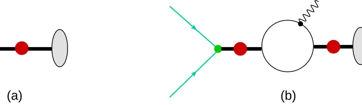
At leading order (LO), only two diagrams (figure 4.1) contribute to the amplitude Y
appearing in equation (4.2). The first is a tree-level diagram and the second involves a one-loop integral.
To start, we first need the interaction vertices, the nucleon and the dressed dibaryon propagators,SN andD, respectively. Fortunately, we have calculated most
(a)
(b)
Figure 4.1 Leading-order (LO) diagrams contributing to the np−→dγ
cross-section. Green solid lines denote nucleons, thick black lines denote dressed dibaryons, and wavy lines denote photons. The small purple circle stands for the photon coupling to the nucleon magnetic moment, and the gray oval for the deuteron interpolating field.
and (3.9). SN and D are given by equations (3.10) and (3.26), respectively. We still
need to compute one more interaction vertex (figure 4.2):
Incoming nucleon to outgoing photon and nucleon:
h N†Am(q)|
ie
2MN
†
(κ0+τ3κ1)~σ·B N~ |Ni= e
2Mqjδkm(κ0+τ3κ1)σiijk, (4.3)
Figure 4.2 Photon vertex
where ~σ·B~ =σiijk∂jAk, ~B =∇ ×~ A~, Am is the outgoing photon field and qj is
the outgoing photon momentum.
4.1
LO calculation of the amplitude
Y
At LO, the amplitudeY appearing in equation (4.2) has a tree-level contribution and a one-loop integral contribution. We will first compute the tree-level diagram (figure 4.1 (a)) and then the one-loop integral (figure 4.1 (b)).
Tree-level contribution: diagram (a) in figure 4.1
The deuteron is in a 3S1 state, and the photon is coupled to the nucleon through a
magnetic interaction vertex. Therefore, the incoming nucleons are in a relative 1S0
state. So we can write
iM(a) = 4 q
Zdε∗ i
(d) (−ig (3S
1) Pi
A0B)NBT
i
(−B)
e
2Mqjδkm(κ0+τ3κ1)σppjk ε
∗m
(γ)NA,
(4.4) where subscripts A’, A and B are spin-isospin indices, andB is the binding energy of the deuteron (also the energy of the outgoing photon). The factor of 4 is a symmetry factor.
Notice that there are two contributions, one fromκ0 and the other from κ1. So, there
will be
(A) PAi0Bτ3κ1σppjk =
1
√
8σ2σiτ2τ3κ1σppjk = √1
8σ2τ2τ3κ1(δip+iiplσl)pjk. (4.5) The δip-term gives
σ2τ2τ3κ1ijk. (4.6)
The second term with the ipl vanishes because
the reason being the Pauli exclusion principle. The κ0 contribution is
(B) PAi0Bκ0σppjk =
1
√
8σ2σiτ2κ0σppjk = √1
8κ0τ2σ2(δip+iiplσl)pjk, (4.8) where theδip-term vanishes because of the Pauli exclusion principle (NBTτ2σ2NA= 0).
The other term contains τ2σ2σi which corresponds to a 3S1 state and when projected
onto the 1S0 initial NN state gives zero.
So the only term that survives is the one appearing in equation (4.6) yielding the following
iM(a) =
4
√
8
q Zdε∗
i
(d) (−ig( 3S
1)) i
(−B)
e
2Mqjε
∗k
(γ)ijkκ1NTσ2τ2τ3N. (4.9)
Upon substitutingg(3S
1)=q 8π
M2r(3S1) and Zd=
r
γr(3S1)
1−γr(3S1), we arrive at
iM(a) =−
2e M s π γ3 1 q
1−γr(3S 1)
κ1ijkε∗
i
(d)q
jε∗k
(γ)(N
Tσ
2τ2τ3N). (4.10)
From equation (4.10), one can read off
Y(a) =
2 M s π γ3 1 q
1−γr(3S 1)
κ1. (4.11)
One-loop contribution: diagram (b) in figure 4.1
The deuteron has spin +1 and orbital angular momentum L = 0. So it’s in a spin triplet state with S = 1. Using the2S+1LJ notation whereS is spin angular
momen-tum,Lis orbital angular momentum, andJ =L+S is total angular momentum, the deuteron state is3S1. In diagram (b) of figure 4.1, the photon couples to the nucleon
via a magnetic coupling σiijk∂jAk which takes away spin angular momentum. Thus
the initial NN state must be in a relative 1S
0. Also both dibaryon-nucleon vertices
before the photon coupling correspond to a 1S
0 state. The cross-section is being
can now write down the expression for the invariant amplitude as
iM(b)= 8 q
Zdε∗ i
(d)[−ig (3S
1)N
A(Pi)ABNB]
e
2MqjδkmN
†
C[(κ0+τ3κ1)σppjm]CDND ε∗ m
(γ)
×
Z d4k
(2π)4
i
[k0−
~k2 2M +i]
i
[k0−B− (~k−B~)2
2M +i]
i
[−k0−
~k2 2M +i]
×[−ig(1S0) N†
E(P † a)EFN
† F]
4π M g2
(1S 0)
i µ+M g42π
(1S0)
∆ [−ig
(1S
0)NTP
aN], (4.12)
where B ' 2.2 MeV is the deuteron binding energy which is taken away by the emitted photon. Thus the photon is also released with linear momentum B~. The factor of ‘8’ is the symmetry factor of diagram (b).
Rearranging some terms we get
iM(b)= 8 q
Zdε∗ i
(d)[−ig (3S
1)(P
i)AB]
e
2Mqjδkm[(κ0+τ3κ1)σppjm]BDε
∗m
(γ)
×
Z d4k
(2π)4
i
[k0−
~k2 2M +i]
i
[k0−B− (
~k−B~)2 2M +i]
i
[−k0−
~k2 2M +i]
×[−ig(1S0) (P†
a)DA]
4π M g2
(1S 0)
i µ+M g42π
(1S0)
∆ [−ig
(1S
0)NTP
aN]
= 8 1 8
q Zdε∗
i
(d) [−ig( 3S
1)] e
2Mqjδkmpjm ε
∗m
(γ)
×
Z d4k
(2π)4
i
[k0−
~k2 2M +i]
i
[k0−B− (
~k−B~)2 2M +i]
i
[−k0−
~k2 2M +i]
[−ig(1S0)]
× 4π
M g2 (1S
0)
i µ+ M g42π
(1S0)
∆ [−ig
(1S
0) NTP
aN]T r[σ2σiσpσ2]×T r[τ2(κ0+τ3κ1)τaτ2]
(4.13)
Three-Propagator Integral:
In order to complete the calculation, we have to evaluate the following three-propagator integral:
I =
Z d4k
(2π)4
1 [k0−
~k2 2M +i]
1 [k0−B−
(~k−B~)2 2M +i]
1 [−k0−
~ k2 2M +i]
(4.14)
would be in the upper-half complex plane. Integrating overk0 gives
I =i
Z d3k
(2π)3
1 [−~k2
M +i]
1 [−~k2
2M −B−
1
2M(~k2−2~k·B~ +B~2) +i]
. (4.15)
After rearranging some terms and neglecting the term B
2
4M in comparison with B
(knowing that B=2.2 MeV and M=940 MeV)we get the integral
I =−iM2
Z d3k
(2π)3
1 [~k2−i]
1 [M B+ (~k− B~
2)2−i]
. (4.16)
The next step is to introduce Fourier transforms f(~r) and g(~r) of the propagators such that
F T[f(~r), ~p] = 1
~
p2−i, (4.17) F T[g(~r), ~p] = 1
M B−~p2−i. (4.18)
In general,
F T[h(~r), ~p] =
Z
d3r h(~r)e−i~p·~r, (4.19) and it can be shown that
g(~r) = 1 4π
e−
√ M Br
r . (4.20)
Taking the limit B −→ 0 in g(~r) gives f(~r) = 41πr. Before I continue with the evaluation of the integral, let me take a few lines to show that
g(~r) = 1 4π
e−
√ M Br
r . (4.21)
In order to do this, we need to insert
g(~r) = 1 4π e− √ M Br r (4.22) into Z
and show that it’s equal to M B+1~p2−i.
Plugging in g(~r) from equation (4.22) into equation (4.23) gives
Z d3r e
−√M Br
4πr e
−i~p·~r =1
2
Z
dr dθ sinθ re−
√
M Br e−iprcosθ
= i 2p
Z ∞
0
dr [e−(
√
M B+ip)r − e−(√M B−ip)r]
= i 2p (
1
√
M B+ip −
1
√
M B−ip) (4.24)
= i 2p (
−2ip M B+p2)
= 1
M B+p2
as claimed above.
We now rewrite the propagators in the integral I in terms of their Fourier trans-forms. So,
I =−iM2
Z d3k
(2π)3[ Z d3r
4πre
−i~k·~r Z d3r 0
4πr0e
−√M Br0e−i(~k−B~
2)·r~0]. (4.25)
This can be rearranged to give
I =−iM2
Z d3k
(2π)3e
i~k·(−~r−r~0) Z d3r d3r0
16π2
1
r e−
√ M Br0
r0 e
iB~2·r~0
. (4.26)
First, we perform the k integration and then the remaining integrations over r and
r0. Notice that the integral over k gives aδ3(~r+~r0).
After integrating over r0 using the Dirac delta function, we get
I =−iM2
Z d3r
16π2
1
r2 e
−√M Br0 e−iB~2·r~0
. (4.27)
Next, we integrate over the angles φ and θ which are both simple integrations to arrive at
I = −iM
2 2πB Z ∞ 0 dr e −γr r sin( Br
2 ), (4.28) where γ =√M B. Using
Z ∞ 0 dr e −γr r sin( Br
2 ) = arctan(
B
we find that
I = −iM
2
2πB arctan( B
2γ). (4.30)
Expanding the arctan [arctan(x) =x− x3
3 +...] and keeping the lowest order term
gives
I = −iM
2
2πB ( B
2γ) =
−iM2
4πγ . (4.31)
Going back to the one loop diagram
For ease of reading, we report below the amplitude expression of Eq.(4.13)
iM(b) = q
Zd ε∗ i
(d) [−ig( 3S
1)] e
2Mqjδkmpjm ε
∗m
(γ) Z d4k
(2π)4
i
[k0−
~ k2 2M +i]
i
[k0−B− (
~k−B~)2 2M +i]
i
[−k0−
~ k2 2M +i]
[−ig(1S0)]
4π M g2
(1S 0)
i µ+M g42π
(1S0)
∆ [−ig
(1S
0)NTP
aN]T r[σ2σiσpσ2]×T r[τ2(κ0+τ3κ1)τaτ2].
(4.32) Now we plugin the value of the three-propagator integral given in Eq.(4.30) into the amplitude expression given above to obtain
iM(b) = q
Zdε∗ i
(d) [−ig (3S
1)] e
2Mqjpjk ε
∗k
(γ) (
−M2
4πγ )[−ig (1S
0)]
4π M g2
(1S 0)
i µ+M g42π
(1S0)
∆ [−ig
(1S
0) NTP
aN] 2δip 2κ1δ3a (4.33)
UsingZd =
γr(3S 1)
1−γr(3S 1), g
2 = 8π
M2r, ∆ = 2
M r(
1
a−µ) andPa=
1
√
8τ2τaσ2, the one-loop invariant amplitude becomes
iM(b) =
2 M s π γ3 1 q
1−γr(3S 1)
γe a(1S0) κ
1 qj ijkε∗ k
(γ)ε
∗i
(d) NTτ2τ3σ2N. (4.34)
From the above amplitude (Eq.(4.34)), we can read off
Y(b) =−
2 M s π γ3 1 q
1−γr(3S 1)
κ1 γ a( 1S
The total amplitude
Y =Y(a)+Y(b)
=− 2
M s π γ3 1 q
1−γr(3S 1)
κ1(γa( 1S
0)−1). (4.36)
4.2
From amplitude to cross-section
The cross-section is given by Eq. (4.1), and the invariant amplitude by equation (4.2) whereY has already been calculated (Eq. (4.36)). The next step is to evaluate|M|2,
so we need the nucleon and proton fields, Nn and Np, respectively. They are given
by
Nn=
1
2(1−τ3)N, (4.37) and
Np =
1
2(1+τ3)N. (4.38) Next, we have
NnTONp =NT
1
2(1−τ3)O 1
2(1+τ3)N, (4.39) where O =τ2τ3σ2. Plugging in equation (4.39) into|M|2 gives
|M|2
=MM†
= [ieY ijkε∗(di)qjε∗(γk)NAT0
1
2(1−τ3)A0A(τ2τ3σ2)AB 1
2(1+τ3)BB0NB0]
×[−ieY abcε∗(da)qbε∗(γc)NC†0
1
2(1+τ3)C0C(τ3τ2σ2)CD 1
2(1−τ3)DD0(N
T)†
D0] (4.40)
where A’, A, B’, B, etc are combined spin-isospin indices carried by the nucleon fields. Using
X
spin,isospin
NAT0(NT)
†
D0 =δA0D0 (4.41)
and
X
spin,isospin
NB0N†
we obtain
X
spin,isospin
|M|2 = e2Y2
16
X
{ijkabcε∗(di)ε(∗da)ε∗(γk)ε(∗γc)qjqb×T r[(1−τ3)(τ2τ3σ2)
(1+τ3)(1+τ3)(τ3τ2σ2)(1−τ3)]}.
(4.43) Next, we use
X
ε(∗di)ε∗(da) = (−δia+
ki
(d)ka(d)
M2
(d)
) (4.44)
and
X
ε(∗γk)ε∗(γc) = (−δkc+
qkqc
q2 ) (4.45)
where k(d) and q are the deuteron and photon momenta, respectively. M(d) is the
deuteron mass.
Since we are calculating the cross-section of unpolarized n(p, d)γ, we will need to average over initial spins which introduces a factor of (1/4). So we arrive at
1 4
X
|M|2 = 1 4
e2Y2
16
ijk
abc(−δia+
ki
(d)k(ad)
M2
(d)
)(−δkc +
qkqc q2 )q
j
qb×4T r[(1−τ3)(τ2τ3σ2)
(1+τ3)(τ3τ2σ2)].
(4.46) After a couple lines of algebraic manipulations, we get to the following expression
1 4
X
|M|2 =e2Y2q2. (4.47)
Knowing that the differential cross-section at threshold is given by (see e.g. Ref. [37])
dσ
dΩ =
γ2+p2
16π2p X
|M|2, (4.48)
where γ2 =M B, B being the binding energy of the deuteron and also the energy of the outgoing photon, p is the momentum of the proton in the center of mass (CM) frame, and M is the nucleon mass.
After substituting equation (4.47) for P|M|2, the total cross-section is σ = 4πe2γ
2+p2
16π2p q
where q = p2M+γ2 is the outgoing photon momentum, which when inserted in the expression above yields the final LO result [32]
σ= α(γ
2+p2)3
M2p Y
2 (4.50)
with α= 4e2π.
Having derived the expression for the n(p, d)γ cross-section (Eq. (4.50)), let us find a numerical value for σLO. Inserting the following:
α = 1371 , γ = √M B ≈ 45.68 MeV = 0.23 fm−1, r(3S1)=1.75 fm, a(1S0)=-23.71 fm, κ1 ≈2.35, p= plab2 = 3.45×10⁻³ MeV (plab =M βlab =Mvlabc with vlab = 2200 m/s)
into Eq. (4.50) where Y is given by Eq (4.36) yields a value of
σLO ≈ 49.4 fm2 = 494 mb (4.51)
Note that since p γ, I have neglected the p2 term in the numerator of Eq. (4.50)
while performing the numerical calculation. Setting c = ~ = 1, we can use 1 MeV=197.13 fm.
Brief discussion of our result
Our LO calculation ofn(p, d)γcross-section using EFT(π/) with dibaryon fields yielded a value ofσLO= 494 mb. This is approximately 1.5 times greater than the
experimen-tal value which is σexp = 334.2 ± 0.5 mb [39]. The energy at which we calculated
the cross-section is 0.025 eV which is the kinetic energy of a thermal neutron. This energy corresponds to the most probable speed of a Maxwell-Boltzmann distribution at room temperature.
The expansion parameter is Q ∼ γ
Mπ where the deuteron binding momentum γ is
a typical momentum scale, and Mπ is the pion mass. The two LO diagrams (Fig.
4.1) contributing to the amplitude Y are of O(Q0). Since our cross-section is a
corresponds to a four-nucleon operator coupling to the magnetic field
e L1
Mqr(1S 0)r(
3S 1)
tj†s3Bj
wheretjandsaare the dibaryon fields in the3S1and1S0, respectively. The coefficient L1 is to be fixed either from QCD or experimentally (see e.g. Ref. [32]). There are
Chapter 5
Conclusion
In this thesis, I have shown the details of the unpolarized n(p, d)γ cross-section cal-culation up to LO employing the framework of EFT(π/) with dibaryon fields. The predicted numercial value is σLO = 494 mb. The cross-section calculation presented
here is only a ‘simple’ application of EFT. Further work using EFTs has been done. The np→dγ cross-section has been calculated to higher orders [1, 2, 3]. The inverse reactions γd→np and~γd→np have also been studied using EFT(π/) with dibaryon fields [3]. Furthermore, EFT has been applied to study the polarizedn(p, d)γ reaction at threshold [4] and parity-violating effects [35, 36].
The n(p, d)γ reaction was put in the context of BBN. The fact that deuterium for-mation is very sensitive to the density of baryonic matter (Ωb) in the universe, its
abundance provides a measure of Ωb (see for example [15]). Deuteron production
cross-section enters in Ωb calculations, so computing this cross-section to higher
pre-cision is a big matter of interest. A prepre-cision calculation of n(p, d)γ cross-section at BBN energies was done by Rupak [2].
Bibliography
[1] J. -W. Chen, G. Rupak and M. J. Savage, Phys. Lett. B 464, 1 (1999) [nucl-th/9905002].
[2] G. Rupak, Nucl. Phys. A 678, 405 (2000) [nucl-th/9911018].
[3] S. Ando, R. H. Cyburt, S. W. Hong and C. H. Hyun, Phys. Rev. C 74, 025809 (2006) [nucl-th/0511074].
[4] T. -S. Park, K. Kubodera, D. -P. Min and M. Rho, Phys. Lett. B 472, 232 (2000) [nucl-th/9906005].
[5] G. Lemaitre, “The Primeval Atom, An Essay on Cosmogony,” New York, Van Nostrand 1950, 186p
[6] R. A. Alpher, H. Bethe and G. Gamow, Phys. Rev. 73, 803 (1948).
[7] S. Weinberg, “The First Three Minutes. A Modern View of the Origin of the Universe,” Muenchen 1977, 269p
[8] R. A. Alpher, J. W. Follin and R. C. Herman, Phys. Rev. 92, 1347 (1953).
[9] M. E. Burbidge, G. R. Burbidge, W. A. Fowler and F. Hoyle, Rev. Mod. Phys. 29, 547 (1957).
[10] A.G.W. Cameron, “Stellar Evolution, Nuclear Astrophysics, and Nucleogenesis” Chalk River 1957, 167p
[11] F. Hoyle and R. J. Tayler, Nature 203, 1108 (1964).
[12] P. J. E. Peebles, Astrophys. J. 146, 542 (1966).
[14] H. Reeves, J. Andouze, W. A. Fowler and D. N. Schramm, Astrophys. J. 179, 909 (1973).
[15] S. Burles and D. Tytler, astro-ph/9803071.
[16] M. Pospelov and J. Pradler, Ann. Rev. Nucl. Part. Sci. 60, 539 (2010) [arXiv:1011.1054 [hep-ph]].
[17] B. Fields and S. Sarkar, astro-ph/0601514.
[18] K. A. Olive, Nucl. Phys. Proc. Suppl. 80, 79 (2000) [astro-ph/9903309].
[19] G. Steigman, Ann. Rev. Nucl. Part. Sci. 57, 463 (2007) [arXiv:0712.1100 [astro-ph]].
[20] S. Burles, K. M. Nollett and M. S. Turner, astro-ph/9903300.
[21] D. B. Kaplan, nucl-th/0510023.
[22] D. B. Kaplan, nucl-th/9506035.
[23] B. R. Holstein, Nucl. Phys. A 689, 135 (2001) [nucl-th/0010015].
[24] H. Georgi, Ann. Rev. Nucl. Part. Sci. 43, 209 (1993).
[25] A. Pich, hep-ph/9806303.
[26] D. R. Phillips, Czech. J. Phys. 52, B49 (2002) [nucl-th/0203040].
[27] M. E. Peskin and D. V. Schroeder, “An Introduction to quantum field theory,” Reading, USA: Addison-Wesley (1995) 842 p
[28] J. C. Collins, “Renormalization. An Introduction To Renormalization, The Renormalization Group, And The Operator Product Expansion,” Cambridge, Uk: Univ. Pr. ( 1984) 380p
[29] J. -W. Chen and M. J. Savage, Phys. Rev. C 60, 065205 (1999) [nucl-th/9907042].
[31] D. B. Kaplan, Nucl. Phys. B 494, 471 (1997) [nucl-th/9610052].
[32] S. R. Beane and M. J. Savage, Nucl. Phys. A 694, 511 (2001) [nucl-th/0011067].
[33] D. B. Kaplan, M. J. Savage and M. B. Wise, Phys. Lett. B 424, 390 (1998) [nucl-th/9801034].
[34] S. Scherer and M. R. Schindler, hep-ph/0505265.
[35] D. B. Kaplan, M. J. Savage, R. P. Springer and M. B. Wise, Phys. Lett. B 449, 1 (1999) [nucl-th/9807081].
[36] J. W. Shin, S. Ando and C. H. Hyun, Phys. Rev. C 81, 055501 (2010) [arXiv:0907.3995 [nucl-th]].
[37] S. Christlmeier, "Electrodisintegration of the Deuteron in Effective Field Theory," Diploma thesis, TU Muenchen (Germany), 2004
[38] G. ’t Hooft and M. J. G. Veltman, Nucl. Phys. B 44, 189 (1972).