Comparative Study of Mixture model and Eulerian Model used in Hydrocyclone
with the help of CFD Simulation
1Indrashis Saha , 2Tathagata Mukherjee
1Department of Chemical Engineering, University of Calcutta, India, Email ID: [email protected] 2Department of Mechanical Engineering, BIT Mesra, India, Email ID : [email protected]
ABSTRACT
Due to the accuracy of numerical calculation of fluid flow inside a hydrocyclone can be obtained using Computational Fluid Dynamics (CFD), highly modified super computers are used to simulate the fluid flow and track particle motion inside a hydrocyclone. This paper deals with the numerical study using three multiphase models viz. Volume of fluid, Mixture and Eulerian model. The dimensions of the hydrocyclone taken into consideration for numerical analysis is same as considered by Rajamani. Validation of axial and tangential velocities at different strategically decided axial stations, RMS axial and tangential velocity profiles of the hydrocyclone is done using Reynolds Stress Model (RSM). The hydrocyclone model has been designed in Creo 3.0 using the same dimensions which later was imported to CFD for meshing. Fine hexagonal mesh numbering up to 5 lacs were constructed to obtain optimum results. Fluid flow was allowed to be developed in ANSYS FLUENT 16.2. Entire simulation took 96 hours to generate results and track particle movements inside the hydrocyclone. The particle tracking has been done using three multiphase model. The first being the volume of fluid was used for validation purposes and the comparison of the Mixture and Eulerian model are the basic focus of this research work. Conclusive results indicate that usage of different multiphase model does not result in variation in particle motion. The slight variation in grade efficiency values are hardly noticeable. The Mixture model and Eulerian model predict lower separation efficiency as compared with Volume of fluid multiphase model.
Keywords- RSM, LES, DNS, Simulation/Numerical investigation, Air-core, Vortex, Grade efficiency
INTRODUCTION
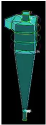
A hydrocyclone is a compact static mechanical structure whore geometry is similar to cylinder incident perpendicularly on a conical structure with small openings at the top and bottom which is technically termed as overflow and underflow (Brennan et al., 2007). Another opening is strategically placed at the upper cylindrical region so that fluid may enter tangentially and form a vortex inside. Feed enters tangentially at high velocity near the top, and the particles follow a spiral path near the vessel wall, forming a strong downward vortex. Air is allowed to enter naturally from the overflow and the underflow which results in the formation of vortex. Large or heavy solid particles separate to the wall because they are not influenced by vortex facing difficulty to follow the tight curve of the stream because of it’s too much inertia. Since these large particles cannot follow the high speed spiral motion, they are hit inside the side walls of the container and are collected in the collection hooper. They are pushed downward of the cyclone as a slurry or paste. A variable discharge orifice controls the overall consistency of the underflow. Most of the liquid particles goes upward by following the stream of the vortex and escapes through the central discharge pipe or the vortex finder. Hydrocyclones are effective pollution control devices and are often used as a pretreatment devices before the flue gas enters. A hydrocyclone has no moving parts and it completely takes advantage of naturally formed centrifugal force inside for the separation of particles (A. Cilliers, 2000). Air is allowed to enter naturally from the overflow and the underflow which results in the formation of vortex. The fluid flow calculations are done in a high end super computer using ANSYS software (E. Macdonald, 2007). The dimensions of the hydrocyclone are kept same as considered by (Rajamani and Delgadilo 2005) and it has been considered as the basic model in which fluid flow has been determined. The basic model of the hydrocyclone has been designed using basic designing software (Creo 3.0) and the simulations were run in ANSYS FLUENT 16.2. The anisotropic flow requires a high-end computer to track its movements. The velocity of the fluid flow is solved using Navier-Stokes equation. Engineers have been using CFD since early 20th century for determining fluid flow trajectories and their velocity profiles which have been helping them to constantly modify and adapt changes to the design of a hydrocyclone to full fill their need (Rajamani and Delgadilo, 2007). There are various ways of solving the Navier-Stokes equation, the most computationally intense yet simplest approach is the Direct Numerical Simulation (DNS) method (Doshi and Dyer 2016). For obtaining good results, high mesh number is recommended. In our study we have considered 5,72,000 (5 lacs) number of mesh. Other than DNS method there are Large Eddy Simulation (LES), Reynolds Stress Model (RSM) and Renormalized group (RNG K-ε) methods also (George G. Chase, University of Akron). We have used RSM approach and Volume of Fluid multiphase model in order to validate the simulated result with the
experimental values, after which the velocity profiles are compared using Mixture and Eulerian model as also used by (Nenu and Yoshide, 2009).
\METHODOLOGY
The hydrocyclone is designed using Creo 3.0 using the same geometry as used by (Hsieh and Rajamani, 1998) and saved in .stp format which is easily recognized in ICEM CFD where it is further imported and meshing has been done. The circular inlet as used in (Hsieh and Rajamani, 1998) has been converted into a square inlet to simplify the meshing procedure. The cross-sectional area of square having each side of 21.02 mm has been calculated in such a so that the total inlet volume is constant in both the cases. First few blocks are constructed all over the basic geometry which are subdivided into a number of nodes leading to the formation of smaller hexahedral mesh (C. Tian et al., 2018).
Figure 1: General block formation of a hydrocyclone in ICEM CFD
The total hydrocyclone has been divided into 5 lacs number of meshes. Along the central axis region, the mesh size is very fine to capture the interface of air and water at the vortex finder region (W.E. Anderson, 2009). The mesh file is saved in. msh format which can be easily imported in FLUENT for further simulation. ANSYS 16.2 has been used for the simulation purpose in this paper. For numerical study flow was at first developed inside the hydrocyclone in STEADY state based on single phase (water) (Karimi, 2012). The simulation was run till 1800 iterations and then it was changed to transient state with multiphase model set as Volume of Fluid. During this stage the Backflow volume fraction of the secondary phase (air) at the overflow and underflow was set at 1, which signifies the entry of air through the outlet pipes naturally (Murthy and Bhaskar, 2012). Time set being set to 5·10-4, simulation was run till 28000 iteration (2.5 seconds) and the air core was perfectly developed. Figure 2 shows the air-core formation within a hydrocyclone. Air-core formation from the underflow till the overflow is clearly visible from left to right as time elapses (A. T. Stephens, 2009). After the formation of air-core, dust particles of density 2700 kg/m2 were injected with particle diameters ranging from 0.5 to 46.9 microns. Total 12220 number of particles were injected at 2.72 m/sec inlet velocity. Figure 2 shows the vector plots and eddy viscosity and other profiles at different planes. The fall of pressure along the central axis is observed in Figure 3(d).
(a) (b) (c)
(d) (e) (f)
(g) (h) (i)
Figure 3: (a) Vortex core, (b) Eddy viscosity at various XY planes, (c) Eddy viscosity at Y plane, (d) Pressure at Y plane, (e) Pressure at various XY planes, (f) Vector (equally spaced) at vortex core
VALIDATION
Before proceeding with the numerical study, the simulated results were compared with the experimental values. Validation of experimented result with numerical study plays a major role in further numerical purpose. The axial velocity, tangential velocity, RMS axial and RMS tangential velocity and are considered for the validation purpose. The velocity profiles are validated at three axial stations viz: 60 mm, 120 mm and 170 mm from the top respectively. The same base models as used in (Delgadilo 2005) was validated using the same working conditions and parameters. At first the velocity profiles are validated.
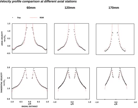
Velocity profile comparison at different axial stations
60mm 120mm 170mm
Figure 4: Velocity profile comparison
The graphs represented in Figure 4, the upper and lower row represent axial and tangential velocities at different axial stations which are 60mm, 120mm and 170mm from the top column wise from left to right. The graphs have been standardized for convenience, with the radial distance along the X-axis is divided by the radius of the hydrocyclone and the velocity values along the Y-axis is divided by the inlet velocity. The circles represent the experimental values while the red dashed line signifies the simulated values as obtained from RSM model approach and the multiphase model being Volume of fluid. The axial velocity profile as obtained from numerical simulation shows resemblance with the experimental values at 60mm and 120mm from the top. The computationally solved values are accurate at the inner and as well as the outer vortex region, while at 170mm from the top, the numerically solved prediction slightly shows unrealistic results outer core while promising result along the inner core. For tangential velocity, the numerically solved graph agrees with the experimental graphs at all the three axial stations. -0.5 0.0 0.5 1.0 1.5 A XI A L V EL O CI TY <w >/ Uin Exp. LES 0.0 1.0 2.0 3.0
-1.0 -0.5 0.0 0.5 1.0
TA NG ENT IA L V EL O CI TY <v >/ Uin x/R RADIAL DISTANCE
-1.0 0.0 1.0
x/R -1.0 x/R0.0 1.0
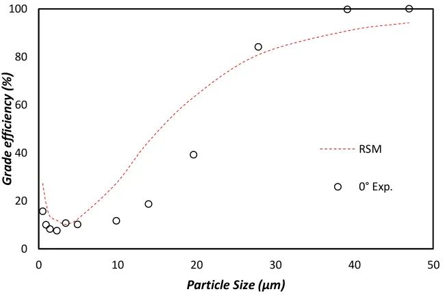
Grade efficiency comparison
The ratio of the number of particles exhausted through the underflow to the number of particles injected through the inlet is known as the grade efficiency. The grade efficiency is determined as to how proficiently particles were distinguished according to size and density. The heavier, hence slightly larger diameter particles get exhausted and collected through the underflow which results in their collection efficiency to almost 90%. Our grade efficiency calculation is based on the number of particles exiting through the underflow.
Figure 5: Grade Efficiency
The numerical solution slightly overpredicts the separation efficiency for particles ranging between 5 to 30 microns as shown in Figure 5. For particles having diameters maximum and minimum are separated efficiently. The larger particles are discharged through the overflow while the smaller particles are exhausted through the overflow. The RSM approach prediction depicts that separation of heavy and light particles is done accurately while on the other hand the separation efficiency of mid-ranged particle sizes is slightly over predicted.
The velocity profiles at the three axial stations as well as the grade efficiency are validated using RSM approach and Volume of fluid as multiphase model. Hence for further numerical study RSM approach with Mixture and Eulerian model as multiphase model is used respectively.
RESULTS AND DISCUSSION
The Volume of Fluid has proven to be a reliable source of numerical values for validation. In this section the velocity profile, both tangential and axial velocity are compared On the second part of the paper, the main focus of the study is to compare the results obtained from Volume of Fluid multiphase model with Eulerian and Mixture model using RSM approach. The results also include comparison of Grade Efficiancy for both the models. All other parameters and working conditions are kept constant during the simulation using CFD.
0 20 40 60 80 100
0 10 20 30 40 50
G
ra
d
e
ef
fi
ci
en
cy
(%
)
Particle Size (µm)
RSM
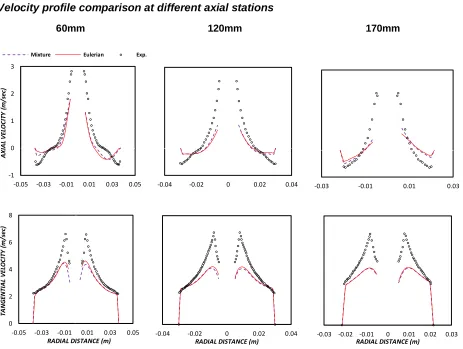
Velocity profile comparison at different axial stations
60mm 120mm 170mm
Figure 6: Velocity profiles for Mixture and Eulerian model
Figure 6 represents the velocity profiles at the three axial stations which were considered during validation. The upper and lower row represent the axial and tangential velocity respectively with the axial stations 60mm, 120mm and 170mm (from the top) left to right. The numerically solved values of the multiphase models (Eulerian and Mixture) highly under predict the velocity profiles at the inner core region. Both Eulerian model and Mixture multiphase model predict very similar results. However, along the inner vortex region the simulated values are highly underpredicted for both axial and tangential velocities. Whereas along the outer vortex region the simulated values for tangential velocity predicts promising results contrary to the axial velocity where numerically solved results are highly over predicted.
Grade efficiency comparison:
Figure 7: Grade efficiency for Mixture and Eulerian method
-1 0 1 2 3
-0.05 -0.03 -0.01 0.01 0.03 0.05
A XI A L V EL O CI TY (m /s ec)
Mixture Eulerian Exp.
-0.04 -0.02 0 0.02 0.04 -0.03 -0.01 0.01 0.03
0 2 4 6 8
-0.05 -0.03 -0.01 0.01 0.03 0.05
TA NG ENT IA L V EL O CI TY (m /s ec)
RADIAL DISTANCE (m)
-0.04 -0.02 0 0.02 0.04
RADIAL DISTANCE (m)
-0.03 -0.02 -0.01 0 0.01 0.02 0.03
RADIAL DISTANCE (m)
0 20 40 60 80 100
0 10 20 30 40 50
G ra d e ef fi ci en cy (% )
Particle Size (µm)
Mixture
Eulerian
Mixture Eulerian
Particle Size Grade Efficiency Particle Size Grade Efficiency
0.5 14.68085 0.5 14.75177
0.9 14.68085 0.9 14.75177
1.4 12.69504 1.4 12.48227
2.3 14.46809 2.3 14.53901
3.4 16.02837 3.4 15.8156
4.9 18.29787 4.9 18.08511
9.8 31.84397 9.8 31.63121
13.9 45.60284 13.9 45.60284
19.6 57.58865 19.6 57.37589
27.8 74.75177 27.8 74.75177
39.1 85.8156 39.1 86.02837
46.9 92.34043 46.9 92.55319
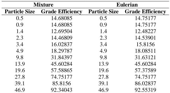
Table 1: Grade efficiency comparison using two different models
Figure 7 is the graph of the grade efficiency of the hydrocyclone considered which is obtained by Volume of Fluid, Eulerian and Mixture multiphase model using RSM approach. The latter two multiphase model predicts unrealistic result for all particles with diameters above 15 microns. The grade efficiency for larger particles is slightly underpredicted. The main observation being the Eulerian and Mixture model predict very similar grade efficiency. There is very small deference in between the graphs obtained by Mixture and Eulerian approach. The exact difference in values obtained after numerical simulation can be further studied in the Table1.The left column of each multiphase model represents the particle diameter whereas the right-side column determines the grade efficiency of the particle sizes. The grade efficiency values are considered up to three decimal places to compare the actual difference in grade efficiencies.
CONCLUSION
The base model used as the dimensions of hydrocyclone has been validated using RSM approach and Volume of Fluid as the multiphase model. The main focus of this study is to compare the results as obtained by using different multiphase model. In this research work the Eulerian and Mixture multiphase model has been used for comparison. The focus being to encourage future engineers to get a brief idea about which multiphase model to use for their study. The numerical simulations conducted in this paper have the same parameters and working conditions as used by Delgadilo just the multiphase model being altered for research purpose. Conclusive result predicts that Mixture model and Eulerian model both results in same grade efficiency as well as velocity profiles. The results obtained by using either of these two multiphase models will not result in much difference in output values. Hence it can be concluded that future researchers can use any of the two procedures based on the requirement keeping in mind that using the other multiphase model will not result in much difference in output values.
REFERENCES
Cilliers, Hydrocyclone for Particle Size Separation, Encyclopedia of Separation Science, (2000)
T. Stephens, J. Mohanarangam, Turbulence model analysis of flow inside a hydrocyclone, Seventh international conference on CFD in minerals and process industries, (2009): 366-373.
C. Tian, J. Ni, O. Song, E. Olson, C. Zhao, An overview of operating parameters and conditions in hydrocyclones for enhanced separation, Separation and purification technology, (2018): 268-285
E. Macdonald, Mineral Process and Design, Handbook of Gold Exploration and Evaluation (2007)
George G. Chase, Solid Notes 11, The university of Akron
J. Delgadillo, R.K. Rajamani, Comparative study of three turbulence-closure models for the hydrocyclone problem, International Journal of Mineral Processing, 77(4),(2005): 217-230
J. Delgadillo, R.K. Rajamani, Large Eddy Simulation of Hydrocyclones, Particle Science and Technology, 25 (2007): 227-245
K. Karimi, W. Akdogan, B. Bradshaw, Mainza, Numerical Modelling of Air Core in Hydrocyclones, ninth international conference on CFD in minerals and process industries, (2012)
M.S. Brennan, M. Narsimha, P.N. Holthman, Multiphase modeling of hydrocyclones-prediction of cut size, (2007): 395-406
N. Murthy, P. Bhaskar, Parametric CFD studies on hydrocyclone, Powder technology, (2012): 36-47
P.Doshi, J.Dyer, Recycling and Recycled Materials, Reference Module in Material Science and Material
R.K.T. Nenu, H. Yoshide, Comparison of separation performance between single and two inlets hydrocyclones, Advanced powder technology, 20 (2009): 195-202