Abstract: In the present work, we provide an electronic structure based method for the “on-the-fly”

Article

“On-the-fly” calculation of the Vibrational

Sum-frequency Generation Spectrum at the Air-water

Interface

Deepak Ojha1and Thomas D. Kühne1,2*

1 _{Dynamics of Condensed Matter and Center for Sustainable Systems Design, Chair of Theoretical Chemistry,}

Department of Chemistry, Paderborn University, Warburger Str. 100, 33098 Paderborn, Germany; [email protected]

2 _{Paderborn Center for Parallel Computing and Institute for Lightweight Design, Paderborn University,}

Warburger Str. 100, D-33098 Paderborn, Germany; [email protected] * Correspondence: [email protected];

Version July 14, 2020 submitted to Molecules

Abstract:In the present work, we provide an electronic structure based method for the “on-the-fly” 1

determination of vibrational sum frequency generation (v-SFG) spectra. The predictive power of 2

this scheme is demonstrated at the air-water interface. While the instantaneous fluctuations in 3

dipole moment are obtained using the maximally localized Wannier functions, the fluctuations in 4

polarizability are approximated to be proportional to the second moment of Wannier functions. The 5

spectrum henceforth obtained captures the signatures of hydrogen bond stretching, bending, as well 6

as low-frequency librational modes. 7

Keywords:vSFG; Air-water interface ; On-the-fly; AIMD 8

1. Introduction 9

Vibrational spectroscopy provides microscopic fingerprints of the structure and dynamics at the molecular level in condensed phase systems.[1–3] However, theoretical interpretation and peak characterization of vibrational spectra predominantly relies on molecular dynamics simulations.[4–9] Nevertheless, the success of simulations also depends largely on the forcefield employed to describe the interatomic interactions. In this regard, ab-initio molecular dynamics (AIMD) has proven to be extremely useful as the interatomic forces are obtained from accurate electronic structure calculations.[10,11] For periodic systems, the overall electronic state within the AIMD framework is generally expressed in the terms of Bloch oribtals

Ψ(r,k) =e(ik·r)ui(r,k), (1a)

where

ui(r,k) =ui(r+R,k), (1b)

withΨ(r,k)being the electronic wavefunction,ui(r,k)the Bloch function andRa translational lattice parameter.[12] An alternative representation, which is more suited for chemical problems, is provided by so-called maximally localized Wannier functions (MLWFs), i.e.wn(r−R)that are obtained by a unitary transformation of the Bloch orbitals.[13,14] The construction of this Wannier representation

Submitted toMolecules, pages 1 – 8 www.mdpi.com/journal/molecules

enables to split the continuously varying total electronic density into contributions originating from localized fragments of the system. Mathematically, MLWFs are expressed as

wn(r−R) = V 2π3

Z

BZdke

−ik·R

∑

Umn(k)ψmk(r), (2)

where R is the lattice vector of the unit cell and V is the real-space primitive cell volume. The J×JmatrixUmn(k)is the unitary transformation matrix andψmk(r)are the eigenstates of the system computed by density function theory (DFT). The corresponding MLWFs are then obtained by the unitary transformationUmn(k)that minimizes the spread functional

S=

∑

Sn=

∑

(Dwn

r

2 wn

E

− hwn|r|wni2). (3)

Therein,

r2

is the second moment, whereashri2is the squared first moment of the Wannier centers. This unitary transformation based localization can be readily implemented on the position operator ˆr within the Wannier representation to obtain localized orbitals for a given periodic system of arbitrary symmetry.[15–17] As a result, the scheme can be used to compute the electronic contributions to the polarization of a system. Moreover, it also allows to calculate instantaneous fluctuations in the molecular dipole moment and within the linear-response regime, obtain the linear as well as nonlinear infrared spectrum using time-correlation function formalism.[18–24] In this regard, Raman and higher nonlinear analogs like v-SFG, 2D-vSFG and 2D-Raman can also be computed by applying a constant periodic electric field using the Berry phase formalism[25–27], or by calculating the polarizability tensorA

Aij=− δMi(E)

δEj

, (4)

where Mis the total dipole moment andE is an externally applied electric field. This scheme of 10

computing the polarizability tensor has been utilized to obtain isotropic Raman spectrum by means of 11

density functional perturbation theory.[28–31] 12

In this paper, we present a novel computational method to obtain the v-SFG spectrum of the 13

air-water interface. This anisotropic Wannier Polarizability (WP) method is based on a technique of 14

computing the fluctuations within the dipole moment and polarizbaility “on-the-fly” during an AIMD 15

simulation without any additional computational cost.[32] For that purpose, the fluctuations in the 16

dipole moment are obtained using the Wannier centers, whereas the components of the polarizability 17

tensor are approximated using the second moment of the Wannier centers. However, it is noteworthy 18

to mention that several other computational studies have obtained the vSFG spectrum using empirical 19

maps[33–40], velocity correlations[41–44], as well as directly from AIMD simulations[45–48]. 20

2. Results 21

2.1. Anisotropic Wannier Polarizability Method 22

the fluctuations of the volume of the Wannier centers instead of the overall molecular volume. As a result, the net isotropic polarizability can be expressed as

¯ A= 1

3 NWF

∑

i=1 Ai =

β 3

NWF

∑

i

S3_i, (5)

whereSiis the spread of theithWannier center,NWFis the number of MLWFs andβis a proportionality 23

constant. The isotropic Raman spectrum is then obtained as the Fourier transform of the polarizability 24

time-correlation function. 25

On similar lines, the v-SFG spectrum of a non-centrosymmetric system is given as

χ2_abc(ω) =

Z ∞

0 dte iωt _˙

Aab(0)·M˙c(t), (6)

whereχ2_abcis the second order susceptibility, whereasAabis theabthcomponent of the polarizability tensor andMciscthcomponent of the dipole moment.[33,36,45] In contrast to Raman spectroscopy, the computation of v-SFG spectra requires the diagonal elements of the polarizability tensor. In this regard, we note that the second moment, i.e.

wnr2

wnand the polarizability are tensors of same size. Accordingly, we have approximated that the component specific fluctuations in the polarizability are proportional to the second moment of the Wannier centers, i.e.

Aab∝

D wn r 2 ab wn E . (7)

The strength of the anisotropic WP method is that for each set of an electron pair, we have a unique 26

Wannier center and its corresponding moments. As a result, the method can be used to specifically 27

study the contributions from the different fragments of the system. Moreover, it is also computationally 28

less expensive as the polarizability is determined "on-the-fly" from the second moments of Wannier 29

centers, which is in contrast with existing approaches, where the polarizability is obtained by numerical 30

differentiation of the total dipole moment with respect to an externally applied electric field. This is 31

to say that a simple minimization of the spread functional provides the Wannier centers and their 32

corresponding moments, which are used to obtain the dipole and the polarizability, respectively. Thus, 33

a single AIMD-based Wannier center calculation is sufficient to obtain the dipole moment, as well as 34

the polarizability. 35

2.2. Application to the Air-water interface 36

To demonstrate the predictive power of the present anisotropic WP method, we have computed 37

the v-SFG of at the air-water interface. For the sake of simplicity, we have assumed that the 38

contributions originating from Wannier centers, which are associated with the lone pair of electrons, to 39

the overall polarizability can be safely neglected. The spectral dynamics is predominantly governed 40

by the dynamical evolution of the Wannier centers corresponding to the bonded electron pairs. The 41

average molecular dipole moment of the water molecules obtained using the Wannier centers, whose 42

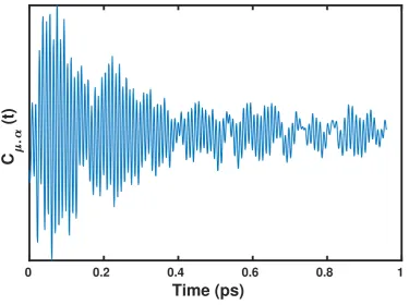
distribution is shown in Fig.1, was found to be 2.46 Debye. The dipole-polarizability cross-correlation 43

function and the v-SFG spectrum computed based on the fluctuations within the dipole moments 44

obtained by using the Wannier centers and polarizabilities by means of the second moment are 45

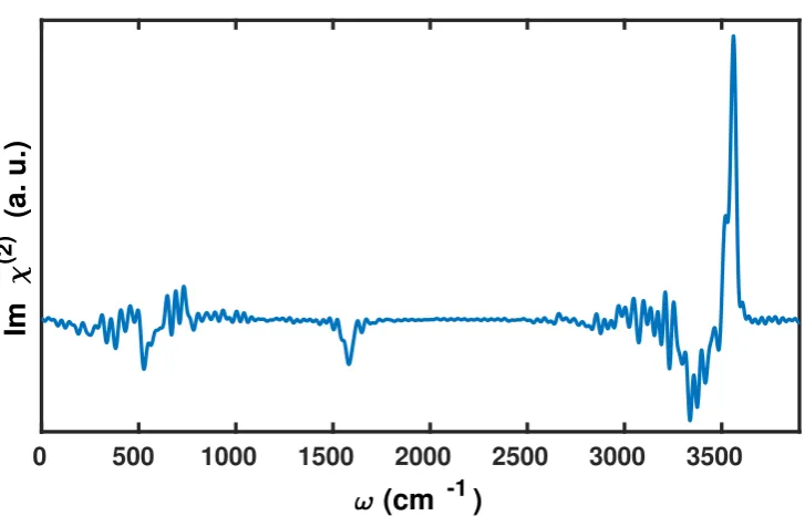
shown in Figs.2and3, respectively. We find that the v-SFG spectrum obeys characteristic peaks 46

corresponding to librational, bending, OH stretching, as well as free OH modes. Since there are 47

various previous experimental and simulation based studies analysing the stretching, bending and 48

librational modes within the v-SFG spectrum at the air-water interface, we only briefly highlight our 49

findings in light of the existing literature. First, we will focus on the spectral region of 3000-3800 50

cm−1, which is predominantly attributed to OH stretching modes. More precisely, earlier simulation 51

1.5

2

2.5

3

3.5

(Debye)

Figure 1. Distribution of molecular dipole moment (µ) of water molecules at ambient conditions, as

computed using the maximally localized Wannier centers.

0

0.2

0.4

0.6

0.8

1

Time (ps)

C

.

(t)

0

500

1000

1500

2000

2500

3000

3500

(cm

)

Im

(2)

(a. u.)

Figure 3. The v-SFG spectrum of interfacial water molecules computed by the present anisotropic WP method.

around 3700cm−1.[33,34,36,37,45] Using our anisotropic WP method, we also find a broad negative 53

peak at 2900-3500cm−1and sharp positive peak around∼3600cm−1. The former broad negative 54

peak contribution originates from hydrogen-bonded water molecules with the overall dipole aligned 55

towards the bulk, whereas the latter sharp positive peak is connected with the free and dangling OH 56

modes of the interfacial water molecules. The observed red-shift within the peak positions can be most 57

likely attributed to the choice of XC functional and employed pseudopotentials in the present study. 58

Earlier experimental and simulation studies of the bending mode have reported a broad negative peak 59

around 1650cm−1and a positive shoulder around 1750cm−1.[43,46] Here, using the anisotropic WP 60

method, we also observe a broad negative peak between 1400 and 1650cm−1, which is governed by the 61

free and dangling OH modes. However, at variance to these earlier studies,[43,46] we can not confirm 62

any positive shoulder in our calculations. Finally, we observe a negative peak at around 450-650cm−1 63

that is governed by the librational motion of water molecules. Apart from a consistent red-shift within 64

the peak positions, our results are in good agreement with earlier results that have also reported a 65

negative peak in the region of 700-800cm−1.[42] 66

3. Computational Methods 67

Ab initiomolecular dynamics simulations were performed by using the method of Car and 68

Parrinello,[10,50] as implemented in the CPMD code[51]. Simulations of the air-water interface 69

comprising of 80 H2Omolecules were performed at 300 K in a cubic box of edge length 12.43 Å 70

corresponding to the density at ambient conditions. [52] The air-water interface was generated by 71

increasing the edge length of the box to 37.2 Å in the z-direction. The Kohn-Sham formulation of 72

density functional theory was applied to represent the electronic structure of the system within a plane 73

wave basis set.[11] In order to represent the core-shell electrons, Vanderbilt ultra-soft pseudopotentials 74

were used and the plane wave expansion of Kohn-Sham orbitals was truncated at a kinetic energy 75

cutoff of 25 Ry.[53] The electronic orbitals were assigned a fictitious mass of 400 a.u. and equations of 76

motion were integrated with a time step of 4 a.u. 77

In the present work, we have used the dispersion corrected BYLP-D exchange and correlation 78

(XC) functional,[54–56] since previous AIMD studies have shown that inclusion of London dispersion 79

diagram of"ab initio"water and aqueous solutions in better agreement with experiment.[48,57–60] 81

The initial configuration was generated using classical molecular dynamics simulations. Subsequently, 82

the production run was carried out in the canonical NVT ensemble using Nose-Hoover thermostats 83

for 50 ps. 84

The identification of interfacial water molecules at the air-water system was conducted using the 85

algorithm for the identification of truly interfacial molecules ITIM.[61,62] This scheme uses a probe 86

sphere to detect the molecules at the surface. The radius of the probe sphere was set to 2 Å which has 87

been proven to be a good value for water.[62] A cutoff-based cluster search was also performed using 88

3.5 Å as a cut-off, which corresponds to the first minimum of the O· · ·O radial distribution function 89

in liquid water. 90

4. Conclusions 91

To summarize, we have proposed a computationally efficient “on-the-fly” method to determine 92

the v-SFG spectrum for interfacial systems. This anisotropic WP method utilizes the second moment 93

of the Wannier centers to estimate the polarizability fluctuations. The major strength of this 94

method is that it captures the spectral signatures of the system for the collective, as well as highly 95

localized modes. Furthermore, it can be directly applied to spectral decomposition by computing 96

fragment-specific contributions from the Wannier centers and their second moment to assist the 97

interpretation of the experimental measurements. Moreover, the algorithm employed here can be 98

easily extended to other spectroscopic techniques like two-dimensional v-SFG,[65] time-dependent 99

v-SFG,[66] 2D-Raman-Thz,[67] pump-probe Thz[68] and 2D-Raman,[69] to name just a few. From 100

the application perspective, interfacial reactivity, “on-water” catalysis, and other interfacial chemical 101

processes can also be studied using our anisotropic WP-based method. Nevertheless, for greater 102

agreement with the experiment, it would be important to better understand the role of simulation 103

protocols and the approximations made, which we propose as an extensions for future works. 104

Author Contributions:D.O. and T.D.K. conceived the methodology, D.O. conducted the simulations, D.O. and

105

T.D.K. reviewed the manuscript.

106

Funding:The authors would like to thank the Paderborn Center for Parallel Computing (PC2_{) for the generous}

107

allocation of computing time on FPGA-based supercomputer “Noctua”. This project has received funding from the

108

European Research Council (ERC) under the European Union’s Horizon 2020 research and innovation programme

109

(grant agreement No 716142).

110

Conflicts of Interest: “The authors declare no conflict of interest.”

111

References 112

1. S. Nihonyanagi, S. Yamaguchi, T. Tahara,Chem. Rev.16, 10665 (2017).

113

2. Q. Du, R. Superfine, E. Freysz, and Y. R. Shen,Phys. Rev. Lett.70, 2313 (1993).

114

3. Y. R. Shen and V. Ostroverkhov,Chem. Rev.106, 1140 (2006).

115

4. H. J. Bakker and J. L. Skinner,Chem. Rev.110, 1498 (2010).

116

5. G. L. Richmond,Chem. Rev.102, 2693 (2002).

117

6. G. L. Richmond,Annu. Rev. Phys. Chem.52, 357 (2001).

118

7. F. Perakis, L. D. Marco, A. Shalit, F. Tang, Z. R. Kann, T. D. Kühne, R. Torre, M. Bonn, and Y. NagataChem. 119

Rev.,116, 7590 (2016).

120

8. D. Ojha, K. Karhan, and T. D. Kühne,Sci. Rep. 8, 16888 (2018).

121

9. C. John, T. Spura, S. Habershon, and T. D. Kühne,Phys. Rev. E93, 043305 (2016).

122

10. D. Marx and J. Hutter,Ab InitioMolecular Dynamics: Basic Theory and Advanced Methods, Cambridge

123

University Press, Cambridge, 2009.

124

11. T. D. Kühne,WIREs Comput. Mol. Sci.4, 391 (2014).

125

12. I. Souza, N. Marzari and D. Vanderbilt,Phys. Rev. B 65, 035109 (2001).

126

13. N. Marzari and D. Vanderbilt,Phys. Rev. B 56, 12847 (1997).

127

14. N. Marzari, A. A. Mostofi, J. R. Yates, I. Souza, D. Vanderbilt,Rev. Mod. Phys. 84, 1419 (2012).

15. P. L. Silvestrelli,Phys. Rev. B 59, 9703 (1999).

129

16. G. Berghold, C. J. Mundy, A. H. Romero, J. Hutter, and M. Parrinello,Phys. Rev. B 61, 10040 (2000).

130

17. R. Resta,Phys. Rev. Lett. 80, 1800 (1998).

131

18. W. Chen, M. Sharma, R. Resta, G. Galli, and R. CarPhys. Rev. B 77, 245114 (2008).

132

19. Marie-Pierre Gaigeot and M. Sprik,J. Phys. Chem. B 107, 10344 (2003).

133

20. M. Heyden, J. Sun, S. Funkner, G. Mathias, H. Forbert, M. Havenith and D. Marx,Proc. Nat. Acad. Sci.107,

134

12068 (2010).

135

21. C. Zhang, R. Z. Khaliullin, D. Bovi, L. Guidoni, and T. D. Kühne,J. Phys. Chem. Lett.4, 3245 (2013).

136

22. D. Ojha, A. Henao, and T. D. Kühne,J. Chem. Phys.148, 102328 (2018).

137

23. D. Ojha and A. Chandra,Phys. Chem. Chem. Phys.,21, 6485 (2019).

138

24. D. Ojha and A. Chandra,Chem. Phys. Lett.,751, 137493 (2020).

139

25. R. Resta,Rev. Mod. Phys. 66, 899 (1994).

140

26. R. D. King-Smith and D. Vanderbilt,Phys. Rev. B 47, 1651 (1993).

141

27. P. Umari and A. PasquarelloPhys. Rev. Lett. 89, 157602 (2002).

142

28. S. Baroni, S. De Gironcoli, A. Dal Corso, and P. Giannozzi,Rev. Mod. Phys. 73, 515 (2001).

143

29. A. Putrino and M. Parrinello,Phys. Rev. Lett. 88, 176401 (2002).

144

30. S. Luber, M. Iannuzzi, and J. Hutter,J. Chem. Phys. 141, 094503 (2014).

145

31. T. D. Kühne et al.,J. Chem. Phys.152, 194103 (2020).

146

32. P. Partovi Azar and T. D. Kühne,J. Comput. Chem. 36, 2188 (2015).

147

33. A. Morita and J. T. Hynes,Chem. Phys.258, 371 (2000).

148

34. A. Morita and J. T. Hynes,J. Phys. Chem. B106, 673 (2002).

149

35. T. Ishiyama, T. Imamura, and A. MoritaChem. Rev.114, 8447 (2014).

150

36. P. A. Pieniazek, C. J. Tainter, and J. L. Skinner,J. Amer. Chem. Soc.133, 10360 (2011).

151

37. Y. Li and J. L. Skinner,J. Chem. Phys.,145, 124509 (2016).

152

38. Y. Li and J. L. Skinner,J. Chem. Phys.,145, 03110 (2016).

153

39. P. A. Pieniazek, C. J. Tainter, and J. L. Skinner,J. Chem. Phys.135, 044701 (2011).

154

40. Y. Li, M. Gruenbaum and J. L. Skinner,Proc. Nat. Acad. Sci.110, 1992 (2013).

155

41. T. Ohta, K. Usui, T. Hasegawa, M. Bonn and Y. Nagata,J. Chem. Phys.143, 124702 (2015).

156

42. R. Khatib, T. Hasegawa, M. Sulpizi, E. H. G. Backus, M. Bonn, and Y. Nagata, J. Phys. Chem. C120, 18665

157

(2016).

158

43. Y. Nagata, C-S Hsieh, T. Hasegawa, J. Voll, E. H. G. Backus, and M. Bonn,J. Phys. Chem. Lett.11, 1872 (2013).

159

44. N. K. Kaliannan, A. Henao, H. Wiebeler, F. Zysk, T. Ohto, Y. Nagata, and T. D. Kühne,Mol. Phys.118, 1620358

160

(2020).

161

45. M. Sulpizi, M. Salanne, M. Sprik, and M. Pierre GaigeotJ. Phys. Chem. Lett.4, 83 (2013).

162

46. R. Khatib and M. SulpiziJ. Phys. Chem. Lett.8, 1310 (2017).

163

47. C. Liang , J. Jeon, and M. Cho,J. Phys. Chem. Lett.10, 1153 (2019).

164

48. T. Ohto, M. Dodia, J. Xu, S. Imoto, F. Tang, F. Zysk, T. D. Kühne, Y. Shigeta, M. Bonn, X. Wu, and Y. Nagata,J. 165

Phys. Chem. Lett.10, 4914 (2019).

166

49. P. Partovi-Azar, T. D. Kühne, and P. Kaghazchi,Phys. Chem. Chem. Phys.17, 22009 (2015).

167

50. R. Car and M. Parrinello,Phys. Rev. Lett.,55, 2471 (1985).

168

51. J. Hutter, A. Alavi, T. Deutsch, M. Bernasconi, S. Goedecker, D. Marx, M. Tuckerman, and M. Parrinello,

169

CPMD Program, MPI für Festkörperforschung and IBM Zurich Research Laboratory. See www.cpmd.org.

170

52. D. R. Lide,CRC Handbook of Chemistry and Physics, 84th Edition. Taylor & Francis, 2003.

171

53. D. Vanderbilt, Phys. Rev. B,41, 7892 (1990).

172

54. A. D. Becke,Phys. Rev. A,38, 3098 (1988).

173

55. C. Lee, W. Yang, and R. G. Parr,Phys. Rev. B,37, 785 (1988).

174

56. S. Grimme,J. Comput. Chem.,27, 1787 (2006).

175

57. M. J. McGrath, I. F. Kuo, and J. I. Siepmann,Phys. Chem. Chem. Phys.,13, 19943 (2011).

176

58. T. D. Kühne, T. A. Pascal, E. Kaxiras, and Y. Jung,J. Phys. Chem. Lett.2, 105 (2011).

177

59. M. J. McGrath, I. F. Kuo, J. N. Ghogomu, C. J. Mundy, and J. I. Siepmann,J. Phys. Chem. B,115, 11688 (2011).

178

60. Y. Nagata, T. Ohto, M. Bonn, and T. D. Kühne,J. Chem. Phys.144, 204705 (2016).

179

61. L. B. Pártay, G. Hantal, P. Jedlovszky, Á. Vincze, and G. Horvai,J. Comp. Chem.29, 945 (2008).

180

62. M. Sega, S. S. Kantorovich, P. Jedlovszky, and M. Jorge,J. Chem. Phys.138, 044110 (2013).

63. K. E. Laidig and R. F. W. BaderJ. Chem. Phys93, 7213 (1990).

182

64. R. F. W. Bader, Atoms in Molecules: A Quantum Theory, Oxford University Press:Oxford (1990)

183

65. J. Bredenbeck, A. Ghosh, H-K Nienhuys, and M. Bonn,Acc. Chem. Res.42, 1332 (2009).

184

66. D. Ojha, N. K. Kaliannan, and T. D. Kühne,Commun. Chem.2, 116 (2019).

185

67. J. Savolainen, S. Ahmed, and P. Hamm,Proc. Nat. Acad. Sci.110, 20402 (2013).

186

68. H. Elgabarty, T. Kampfrath, D. J. Bonthuis, V. Balos, N. K. Kaliannan, P. Loche, R. R. Netz, M. Wolf, T. D.

187

Kühne, and M. Sajadi,Sci. Adv.6, eaay7074 (2020).

188

69. Y. Tanimura and S. Mukamel,J. Chem. Phys.,999496 (1993).

189

c

2020 by the authors. Submitted toMoleculesfor possible open access publication under the terms and conditions

190

of the Creative Commons Attribution (CC BY) license (http://creativecommons.org/licenses/by/4.0/).