1
The and the Seven Events in Hong Kong: A New Look at Return Synchronicity and Price Efficiency
Jinghan Cai, Fengyun Li, Iordanis Petsas1
This paper identifies a dilemma in the relationship between and price efficiency: After
comprehensively studying the change around 7 well-known corporate events, neither the
traditional understanding of as price inefficiency, nor the behavioral way of as price
efficiency can explain the observed change around the events. We adopt an alternative
methodology to replace the standard difference-in-difference regression and directly decompose
the change. We find that, due to the endogeneity of events, the changes of are
over-estimated. We further propose that in the event study setting, the change may be simply the
consequence of the inflow/outflow of some trend-chasing investors, and it may be detached from
price (in) efficiency. Empirical evidences are consistent with this hypothesis.
Introduction
The of a stock is derived from regressing the stock’s returns on one or multiple market indices
or common factors. Academia’s attention on can date back to Roll (1988), who finds a low ,
implying high firm-specific return variations, is driven either by private information or simply
noise unrelated to specific information. French and Roll (1986) note that the key distinction
between public and private information is that public information affects prices the moment it
becomes known, while private information is only revealed through trading. Subsequently, Morck,
Yeung and Yu (2000) (MYY hereafter) start a large body of research on . They propose that
stronger property rights promote informed arbitrage, which capitalizes detailed firm specific
information. Therefore, is a measure of inverse price informativesness. This -based
inefficiency measure has gained increasing popularity in recent years and is widely used in various
1Jinghan Cai and Iordanis Petsas are from Department of Economics and Finance, University of Scranton. Fengyun
empirical studies of corporate investment and emerging market development, e.g., Wurgler, (2000),
Durnev, et al. (2004), Durnev, Morck, and Yeung (2004), Jin and Myers (2006).
In contrast to the standard wisdom as stated by MYY, there indeed exists the opposite
understanding of the relationship between and price efficiency. Hou, Peng and Xiong (2013)
(HPX hereafter) argue that if stock price fluctuations are driven by investor overreactions, lower
return is associated with stronger medium-term price momentum and long-term price reversal,
two commonly believed signs of market inefficiency. In short, the sentiment-driven (retail)
investors would react and result in a positive relationship between and price efficiency. Along
this line, many papers have also provided supporting evidences (Kelly, 2014, Thoh, Yang and
Zhang, 2007 among others).
In this paper, we argue that more attention should be paid when is applied as either a measure
of price inefficiency, or a measure of price efficiency, especially in the event studies. The
motivation is driven by two well-studied events in the literature: stock splits and the lift of
short-selling constraints. In the literature, stock splits are proved to be related with a larger investor base.
Due to the influx of uninformed investors, who also tend to be small retail investors2, after the
splits, the liquidity improves, trading becomes more active, and the probability of informed trading
decreases, implying a lowered price efficiency. If one believes in the MYY explanation that is
a price inefficiency measure, it is not surprising to see that Chang, et al (2015) find out that
increases after the splits.
Another corporate event that draws our attention is the removal of short sales constraints. As
Morck, Yeung and Yu (2013) articulate, “(some) countries ban short selling, presumably reducing
the value of roughly half of all nonpublic information.” In other words, the existence of short sales
bans excludes a large chunk of the information from being impounded into the stock prices.
Therefore, not surprisingly, when the short sales bans are removed, the price efficiency will
improve. Both theories (Diamond and Verrechia, 2003) and empirical results (Chen and Rhee,
2013, among others) find unanimously consistent results (i.e., after the removal of short sales
constraints, the price becomes more informative).
Based on these observations, if again we believe in MYY’s explanation, we would predict that the
would decrease. However, in a recent paper, Cai and Xia (2014) use the Hong Kong Stock
market data and document that the actually increases after the removal of short sales constraints.
Cai and Xia are not alone: A more recent paper, Kan and Gong (2017), uses the SHO pilot program
in the U.S. market, and finds similar results as in Cai and Xia (2014). These papers in the literature
put the understanding of and price inefficiency into a dilemma. Neither the MYY’s
interpretation nor the HPX’s can explain the conflicted results between the splits and short selling
constraints events raised above.
In this paper, we apply Hong Kong Stock Market data, and adopt seven corporate events (stock
splits, revers splits, addition to Hang Seng index, deletion from Hang Seng index, allowing short
selling, banning short selling, as well as rights offerings) to give a comprehensive examination
about the empirical relationship between and information. Specifically, we re-examine how the
will respond to these 7 events, since in the literature, there are some empirical papers that
provide opposite evidences compared with Chang et al (2005) and Cai and Xia (2014), Kang and
Gong (2017)3. We would like to firstly assure Chang/Cai/Kan results are robust enough to exhibit
the existence of the dilemma. Then, we extend the exploration to other corporate events. Initially,
we indeed find the following results as shown in Table 1, which are consistent with the literature.
(Insert Table 1)
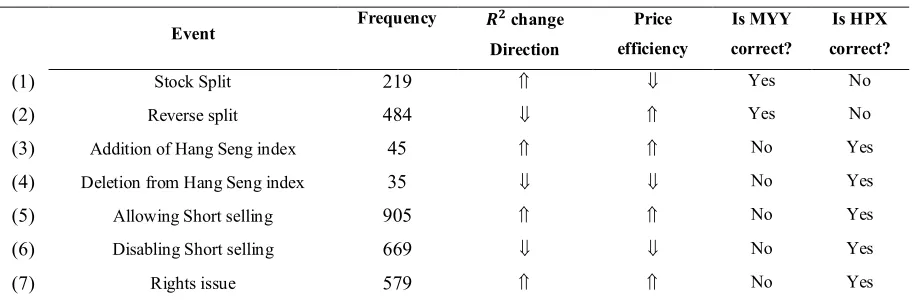
Moreover, the results in Table 1 indicate that the said dilemma indeed exists: The and price
efficiency movements are not consistent within these seven events. Neither MYY nor HPX can
explain what happens around these events. We therefore suggest that researchers should be careful
when adopting to represent either the price inefficiency or the price efficiency, at least under
the event study context.
We try to reconcile the seemingly discordant results in two ways: first, we identify an endogeneity
problem of the timing for the events, which leads to an over-estimated change. After controlling
for the endogenous timing of the events, only 4 out of the above 7 corporate events have robust
changes. Second, we provide the following behavioral explanation: The increase (decrease)
exhibited above may simply be due to the inflow (outflow) of the investors who are more “indexed”
traders.
First, none of the above seven events are purely exogenous. Firms may choose to proceed with
these events at different market conditions. For example, more firms may tend to split their shares
when market goes up, and they are more likely to consolidate (reverse split) the shares when the
market goes down. Another example is, the Hong Kong Stock Exchange puts more firms in the
shortable list in the bull market, but more firms are removed from the list in the bear market. It is
obvious that the seven events are endogenous decisions, depending on the market condition. Based
on these facts, we use a probit model and figure out that the -increase events (split, addition to
Hang Seng Index, allowing short selling and rights issuing) are more likely to occur when the
market return goes up and the market return volatility is low, and the -decrease events (reverse
split, deletion from Hang Seng Index, banned short selling) are more likely to occur when the
market return goes down and the market return volatility is high. Subsequently, in the post-event
window of the -increase events, market returns and volatility reverse, and we observe lower
market returns and significantly higher market volatility. In parallel to that, in the post-event
window of the -decrease events, we observe higher market returns and lower market volatility.
The market change is unlikely to be the results of the events, rather, it comes from the endogenous
timing of the events. The consequence of the endogeneity problem is that, the changes might
be significantly over-estimated. We decompose the changes and find out that a large fraction
of the change comes from the market volatility change, rather than any firm-specific factors. After
we control for the market change, we find no significant changes around allowing/banning
short selling, or around rights offerings. So, our following discussions are based on the events of
stock split/consolidation, addition to/deletion from Hang Seng Index.
In order to control for possible endogeneity issues, one standard methodology is to choose a control
group as benchmark, and use methods like difference-in-difference regressions (DID). However,
we argue that, despite of the popularity of DID, it is not impeccable in the procedure of selecting
the control stocks. While controlling for the market change, it is possible that some control groups
group, and figure out that around some events, the control stocks exhibit significant changes
due to some unknown reasons. Therefore, the DID procedure actually uses some biased bench
mark. Our method avoids this potential drawback of DID.
In our explanation about the changes, we argue that the investor composition around the
above-mentioned events. In the case of stock splits, lowered price would result in a larger investor base,
and more retail investors are attracted into trading the split stock. According to Nofsinger (2014),
retail investors tend to be more active when index return goes dup, implying that retail investors
are more “indexed” investors, compared with other investors. Using Chinese stock market data,
Cai, He, He and Zhai (2018) actually find out that the retail investors’ participation positively
commoves with the market on an event study basis, which gives direct supports to our paper.
Therefore, when firms split (consolidate, or reverse split) their shares, their investor base increases
(decreases), and more small retail investors enter (leave) the stock, accompanied by the increase
(decrease) of .
Another event is the addition to/deletion from the Hang Seng Index. The vast popularity of Hang
Seng index-linked investment products, such as mutual funds, futures, and options, suggests that
the index is a preferred habitat for some investors and a natural category for many more. When a
stock is added to the Hang Seng index, it enters a category (habitat) used by many investors and is
buffeted by fund flows in and out of that category (habitat). If arbitrage is limited, these fund flows
raise the correlation of the included stock’s return with the returns of other stocks in the Hang Seng
Index, and thus, become more (less) synchronous of the index, leading to a higher (lower) .
Moreover, according to Chen, Singal and Noronha (2005), addition to major stock index leads to
a higher level of investor awareness, which also attracts more retail investors. The tends to
increase (decrease), correspondingly.
In short, our above stories argue that the change may reflect the change of investor composition,
which may not necessarily be related to price efficiency. If our above stories about different types
of corporate events and their potential impact on are true, we would observe that the trading
and indeed find a positive co-movement beween and trading volume. This result provides
consistent evidence supporting the investor composition hypothesis of .
The rest of the paper is arranged as follows. Section 2 reviews the literature. Section 3 shows the
data, and basic information of Hong Kong Stock market. Section 4 discusses the empirical results,
and section 5 concludes.
2. Literature Review 2.1
Whether is a proxy of price efficiency or noise? Ever since MYY, evidences have been
mounting on both sides of the discussion. On the one hand, following French and Roll (1986) and
Roll (1988), firm-specification fluctuation reflects more than just public news, and they credit
private arbitrage for much stock price fluctuation. Higher firm-specific variation in higher-income
countries might reflect arbitrageurs’ falling costs or rising trading revenues. As discussed in Morck,
Yeung and Yu (2013), tends to be low after emerging markets lower inward foreign portfolio
investment barriers (Li et al. 2004); receive increased equity investment inflows from the United
States (Bae, Bailey and Mao 2006); announce stock market liberalizations (Bae, Bailey and Mao
2006); or allow cross-listings or closed-end country funds into the United States, the United
Kingdom (Bae, Bailey and Mao2006), or Hong Kong (Gul, Kim and Qiu 2010). These findings
also fit the pattern if foreign arbitrageurs raise the intensity and sophistication of informed trading.
On the other hand, another stream of literature shows that higher is correlated with higher price
efficiency. For example, Gassen, Skaife and Veenman (2017) find that much of the differences in
both within and across countries is driven the differences in liquidity, subverting findings in
prior research suggesting that stocks’ low s result from transparent information environments.
HPX provide evidence consistent with greater pronounced overreaction-driven price momentum
among low- stocks. Dasgupta, Gan and Gao (2010) provide both theory and evidence that
can increase when transparency improves. Chan and Chan (2014) investigate the SEOs as events
Some seemingly contradicted empirical findings can be reconciled if we scrutinize the cost of
information production industry. In a dynamic model with discrete fixed costs of information
gathering and processing, Veldkamp (2006) uses a dynamic model with discrete fixed costs of
information production and argues that competition biases information suppliers toward producing
information useful for estimating the fundamental values of many firms because this has more
buyers than information about one stock. Higher fixed costs of information production extenuate
this, leading to even less production of information about individual firms. Thus, where arbitrage
fixed costs are higher, more investors trade en masse on the basis of the same information about
the same subset of stocks, rendering returns more synchronous. For example, Piotroski and
Roulstone (2004) find that stocks followed by more analysts comove more in the United States.
Chan and Hameed (2006) find similar results in emerging markets. All these findings can be
understood within the context of Veldkamp (2006) that analysists’ forecasts contain information
about industry or economy-levels. However, Veldkamp (2006)’s model is still silent on other firm
specific event studies which are unrelated with information production cost (e.g., stock splits).
Two papers consider the relationship between and liquidity, which are similar to our paper’s
arguments. Chan, Hameed and Kang (2013) discuss the “relative synchronicity” hypothesis which
predicts that stock return co-movement, or the measure, positively affects the liquidity of a
stock, as market makers learn more information from the market if the stock has more correlated
fundamentals. They provide evidence that stock price synchronicity affects stock liquidity
positively. Also, they find that improvement in liquidity following additions to the S&P 500 Index
is related to the stock's increase in return co-movement. In short, Chan, Hameed and Kang (2013)
argue that increase would lead to an improved liquidity. However, unlike the addition to index
events, other events in our paper, such as the stock split/reverse split events are not related with
any fundamental changes. Therefore, other theories of the positive correlation between and
liquidity are needed. Our empirical results that are positively correlated with trading volume,
are consistent with theirs, but we provide an alternative explanation that this may be the evidence
2.2 Stock split
Why do firms bother to take actions to split, or to consolidate (reverse split) its outstanding shares?
The trading range hypothesis (see Copeland, 1979, Lakonishok and Lev, 1987) argues that the
management would like to bring the stock price into a certain optimal range and hence the stability
and liquidity of the stock will improve after a split due to an increase in the ownership base. Merton
(1987) argues that a larger investor base will result in a higher firm value by reducing cost of
capital, ceteris paribus. Empirical studies find supportive evidence that firms that take actions to
expand their shareholder base indeed benefit from a low cost of capital (e.g., Grullon, Kanatas,
and Weston, 2004, among others). Existing literature further ascertains that a larger investor base
would lower the price informativeness. For example, Peress (2010) argues that the extent to which
investors are encouraged to acquire firm-specific information depends on the size of shareholder
base. The intuition is that the enlarged investor base increases risk sharing by spreading the risk
among a large number of investors. As investors’ expected losses decrease, they have less
incentives to gather information with respect to the uncertainty about firm payoff. In other words,
information production in general is negatively related to the degree of risk sharing. Empirically,
Guo, Zhou and Cai (2008) use Tokyo Stock Exchange data and find out that the stock splits tend
to increase the trading activity, to enhance the market liquidity, to reduce the information
asymmetry, and to lower the probability of informed trading. Using 5,104 NYSE/AMEX/Nasdaq
stock splits from 1994 to 2007, Chang et al (2015) find that the adjusted Probability of INformed
Trading (adjPIN, see Duarte and Young, 2009) decreases significantly after stock splits, also
supporting the prediction that stock splits will result in lower price efficiency.
2.3 Addition to Index
The act of adding a stock to the major index should not change investors’ perceptions of the
covariance of the included stock’s fundamental value with other stocks’ fundamental values. The
stated goal of an index is to represent the market’s economy, not to signal a view about future cash
flows. However, deletions from the index are another matter. Stocks are usually removed from the
index because a firm is merging, being taken over, or nearing bankruptcy. There might be some
The major stock index in Hong Kong Stock market is the Hang Sang index. The traditional wisdom,
derived from economies without frictions and with rational investors, holds that the price
synchronicity with the market should not change, since addition to the Hang Seng index does not
change the cash flows of the firm. On the other hand, as argued in Barberis, Shleifer and Wurgler
(2005), in economics with frictions or with irrational investors, and in which there are limits to
arbitrage, comovement in prices is delinked from comovement in fundamentals. This suggests a
second broad class of “friction-based” and “sentiment-based” theories of comovement. Barberis,
Shleifer and Wurgler (2005) examine three specific views of comovement that can be described
in these terms. The first is the category view, analyzed by Barberis and Shleifer (2003). They argue
that, to simplify portfolio decisions, many investors first group assets into categories such as
small-cap stocks, oil industry stocks, or junk bonds, and then allocate funds at the level of these categories
rather than at the individual asset level. If some of the investors using categories are noise traders
with correlated sentiment, and if their trading affects prices, then as they move funds from one
category to another, their coordinated demand induces common factors in the returns of assets that
happen to be classified into the same category, even when these assets’ cash flows are uncorrelated.
Another kind of comovement is the habitat view, starting from the observation that many investors
choose to trade only a subset of all available securities. Such preferred habitats could arise because
of transaction costs, international trading restrictions, or lack of information. As these investors’
risk aversion, sentiment, or liquidity needs change, they alter their exposure to the securities in
their habitat, thereby inducing a common factor in the returns of these securities. This view of
comovement predicts that there will be a common factor in the returns of securities that are held
and traded by a specific subset of investors, such as individual investors.
In both cases, when a stock is added to the Hang Seng index, it enters a category (habitat) used by
many investors and is buffeted by fund flows in and out of that category (habitat). If arbitrage is
limited, these fund flows raise the correlation of the included stock’s return with the returns of
other stocks in the Hang Seng Index, and thus, become more (less) synchronous of the index,
2.3 Short selling ban
Short selling bans have been widely studied starting from Miller (1977), who argues that
short-selling bans drive up the price because holders of negative information are kept out of the market.
Harrison and Kreps (1978) follow Miller (1977) and construct a model to show that when the
short-selling constraints are binding, a stock can be overvalued. Diamond and Verrecchia (1987)
predict that a short sale ban widens the bid-ask spread, thereby suggesting a negative liquidity
effect. Correspondingly, Marsh and Payne (2012) find a deterioration in liquidity, trade, and
market quality in the shorting ban in the 2008 financial crisis period in London. Beber and Pagano
(2013) find that a ban causes a deterioration of liquidity and a slower speed of price discovery.
Boehmer, Jones, and Zhang (2013) find that large American stocks experience a decline of trades,
wider bid-ask spreads, and lower liquidity conditions from August to October 2008. All these
above studies confirm that the negative liquidity effect remained true in the urgent and somewhat
discretionary shorting bans during the 2008 crisis. However, some other papers provide different
opinions: Zhang and Ikeda (2017) and Cai, Ko, Li and Xia (2018) use the case of Hong Kong
Stock Exchange and find out that the liquidity may get better after short selling is banned (and
liquidity worsens after the lift of short selling ban). Cai, Ko, Li and Xia (2018) argue that this is
due to the fact that retail investors leave the market when short selling is allowed. According to
the above results, the impact of short selling ban on liquidity is ambiguous.
2.3 Rights offerings
Rights offerings are one of the major ways for Seasoned Equity Offerings (SEOs), but they are
also minimally studied (Holderness and Pontiff, 2016). In a rights offering, existing shareholders
are given the right, but not the obligation, to purchase newly issued securities which are
proportional to their fractional ownership in the firm. In comparison to rights offerings, another
way of SEO, known as public placement, refers to selling the new shares to the public. However,
unlike public placements, rights offerings may cause value-destructive effects. For example, Wu
and Wang (2002) find negative cumulative abnormal returns after rights offerings. However,
existing evidence, e.g., Balachandran et al (2013), argues that high quality firms tend to issue rights
offerings. How different investors will respond to rights offerings? This question remains unclear
3. Hong Kong Stock market and the data
In this paper, we choose Hong Kong Stock Market for at least the following reasons. First, Hong
Kong stock market provides a good case where a variety of corporate events can be found,
including stock splits, reverse splits, addition to/deletion from Hang Seng Index, etc. More
importantly, Hong Kong has a unique mechanism of short selling. Hong Kong Stock Exchange
(HKEx) allows short-selling of stocks if they are on the designated list. The list is adjusted
quarterly, therefore, we can have a series of events where some stocks are added to the list while
others are deleted from the list. This mechanism differs from any other events of short selling
around the world, in the sense that, in other markets (U.K, U.S, etc.) the short selling bans are most
likely the passive results due to the threat from financial crisis. In the U.S. market, the Regulation
SHO pilot program is an exception, which removed short-selling price tests for randomly-selected
stocks (“pilot stocks”) in May 2005, before removing such tests for all stocks in July 2007.
However, the SHO pilot program occurs at one time slot, which is essentially one single event,
which is not an ideal setting. Moreover, Hong Kong has many cases of rights offerings, which are
relatively rare in U.S. stock market.
In this paper, the information of the events about stock split, reverse split and rights offerings are
provided by HKEx. The sample period is from January 1996 to December, 2016. 559 reverse split
events and 236 split events are identified, and 765 rights offerings are identified. The Hang Seng
Index addition/deletion events are from Hang Seng Indexes Company Limited website4. The
sample period is from January 1995 to December, 2017. There are 49 deletion events, and 66
addition events. The short-selling status change data are from HKEx5. The sample period is from
January 1996 to December, 2008. There are 812 deletion events and 1150 addition events. The
individual stock information is from Datastream. We use the local code (LOC) item from
Datastream to match the events and the individual stock data. For an above event, we use the
[-120 trading days, announcement date] as the pre-event window, and [effective date, [-120 trading
days] as the post-event window. Moreover, in order to remain in our sample, we require that there
are no fewer than 60 observations in either the pre- or post-event window. The final number of
events used in our sample is shown in Table 1.
4https://www.hsi.com.hk/HSI-Net/HSI-Net
4. Empirical Results 4.1 The change of
We start with the direct comparison for the between the pre- and post-windows for the seven
events. Using the 120-day window around the events, we run the following market model
∈ { , } = + + , t=1, 2,…, (1)
where is the continuously compounded return for stock-event i on day t, if t is in window j (pre-
or post-event window), is the Hang Seng index return on day t, and is the error term. is
the total number of observations for stock-event i in window j={pre, post}. The is then
=
+
(2)
where is the beta value estimated from equation (1), is the market return variation measure
for stock-event i, from window j, and more specifically, = ∑ ( − ) , and
is the sum of squared residuals for stock-event i, from window j. For simplicity’s sake, we omit
the subscripts when there is no confusion. For each stock-event, we have one pre-event window
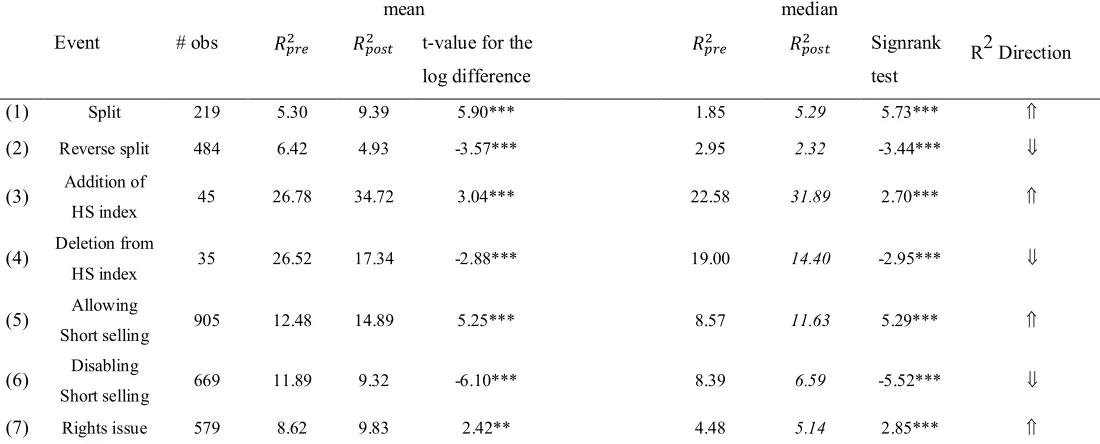
, and a post-event window one. Table 2 shows the direct comparison between the mean and
median of the for pre- and post-event windows.
(Insert Table 2)
We can see from Table 2 that, consistent with the existing literature, we do fine significant
increases in mean or median after stock splits, addition to Hang Seng Index, allowing short selling
and rights offerings. Correspondingly, the decreases significantly after the events of reverse
splits, deletion from Hang Seng Index, and banning short selling. The results are highly consistent
4.2 Endogenous timing of the events
It is not surprising that the above seven events are not strictly exogenous. In the literature, the
standard way to get rid of the endogeneity problem in an event study is to select a control group
and run a difference-in-difference regression (DID). In this paper, we use an alternative method
that can directly calibrate the subsequent impact from the market. To begin with, we first test the
endogeneity of the seven events by directly running the following probit regression:
( ) = + + + (3)
where Prob(1) is a dummy variable which equals 1 if event i leads to increase, including stock split, addition to Hang Seng index, allowing short selling, and rights offerings, and 0 if event i
leads to decrease, including stock consolidation, deletion from Hang Seng Index and disabling
short selling. is the average daily Hang Seng Index return for stock-event i in the
pre-event window; and is the Hang Seng Index return standard deviation for stock-event i in
the pre-event window. is the error term. The results are shown in Table 3.
(Insert Table 3)
Equation (3) embeds the null hypothesis that the events themselves are purely exogenous, and they
are not subject to the impact of the prevailing market condition. However, the results from Panel
A, Table 3 shows that, firms are more likely to split their shares, to be added to Hang Seng Index,
to be allowed to short selling, and to conduct rights offerings when the market return is higher and
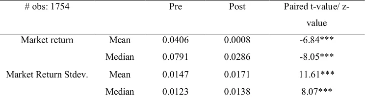
the market volatility is lower. The results are significant. We further examine the comparison of
market return and volatility between the pre-event and post-event window. The results are shown
in Panels B and C of Table 3. We can see that there are reversals in both return and volatility. After
the increase (decrease) events, the market returns are significantly lower (higher), and the
market volatilities are significantly higher (lower). It is very unlikely that the individual stock
events would significantly impact the market, therefore, the reason of this return/volatility reversal
may come from the timing of the events. However, as a result, the endogeneity of events will lead
4.3 Decomposition of change
In our paper, we directly decompose the change and examine the magnitude of the endogeneity
problem.
We know from earlier discussion that the market-model is constructed as follows:
=
+
(4)
where is the beta value estimated from regressing the individual stock return on the market
return, V is the market return variation measure, more specifically, = ∑ ( − ) ,
where is the market return on day t, t=1, 2,…,T, and SSE is the sum of squared residuals. For
simplicity’s sake, we omit all the subscripts.
After a log-linearization, the change is approximately (see appendix for a detailed explanation
of the procedure):
= + − ∗ − (1 − ∗)
(5)
where the tilde expression in equation (5) is defined as follows: for a variable x, = ∗∗, or the
percentage deviation of about ∗, where ∗ is the steady state value of x. In equation (5), we use
the pre-event window as the steady state. The results of the decomposition are shown in Table 4.
(Insert Table 4 here)
In Panel A of Table 4, we can see that, the increase events lead to 15.39% higher . The steady
state ∗=10%, = −20.82%, which leads to a reduction . = 35.86%, therefore ∗
is close to zero and can be neglected. (1 − ∗) = (1 − 10%)4.19%=3.77%. The above
decomposition shows that, the majority of increase is from the market return variation . We
can decompose the decrease in Panel B of Table 4 analogously, and about half of the
variation plays an important role in explaining the change, and the change due to the
firm-specific event is over-estimated.
4.4 The design of
The standard methodology to control the endogeneity problem in an event is the
difference-in-difference regression (DID). However, DID is not impeccable, in the sense that, first, DID is not
able to directly calibrate the impact from the market, and second, while removing the market wide
factors, the sample-specific properties of the control group will be attributed to the test group, so
that some extra errors may occur. In our paper, we adopt a new methodology that fixes the market
impact in the estimation of the change. We name this fixed version of the “fixed- ”, or
, for short. For stock i, , , is defined as follows:
, , =
, , =
, ,
, , + ,
, =
V is the market return variation measure, more specifically, = ∑ ( − ) , where
is the market return on day t, t=1, 2,…,T, and SSE is the sum of squared residuals. The logic of
is, in the post-event window, we use the pre-event market variation to replace the post-event
value, so that there is no market variation difference. By using this alternative method, we are able
to (1) calibrate the magnitude of the endogeneity problem, and (2) to prevent any
control-sample-specific errors, which is explained in Table 5.
(Insert Table 5)
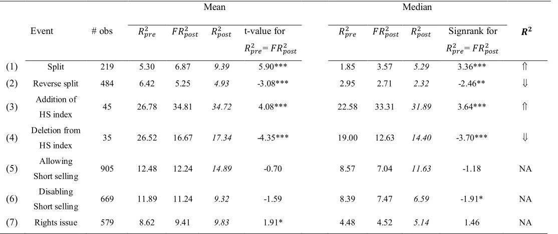
Panel A of Table 5 shows the comparison around the seven events between the standard and
fixed- ( ). We can see that, in most of the increase events, the standard post-event ,
i.e., tends to be over-estimated. For example, in the stock split case, the standard is
to that, for the decrease events, the tends to be under-estimated. For example, in the
reverse split case, the is 4.93%, while the is only 5.25%. Based on the fixed- , we
re-examine the change around the seven events, and figure out that allowing/banning short
selling and rights offerings do not result in significant change in the fixed- at 5% level. The
observed the change (see Table 2) is therefore from the change in market volatility. In
comparison to that, the stock split/reverse split, addition to/deletion from Hang Seng Index events
still have significant impact on the . Therefore, in the rest of the papers, we will focus on the
mechanism of these four events.
Panel B of Table 5 shows the comparison around between the standard and fixed- ( )
for a control group. In finding out the control group, we match the price, market value and trading
volume for a stock-event in the test group from the same industry6. We can see that, the match is
effective, in the sense that the selected control group stocks show similar magnitudes of . Also,
for 5 of the 7 events, there are no significant changes in fixed- around the events. However, for
banning short selling and rights offerings events, there are significant differences in the
fixed-around the events, due to some unknown reasons. If standard DID is applied, these changes would
be attributed to the attributed to the test group. The results from Panel B of Table 5 provide
evidence for the potential drawbacks of DID, and our methodology is free of this issue.
4.5 A behavioral explanation of the change
We have shown that the stock split and addition to Hang Seng Index would lead to a significant
increase in , while the reverse split and deletion from Hang Seng Index would lead to a
significant decrease. Instead of explaining the findings from the perspective of price efficiency or
inefficiency, we tackle this question from the angle of investor composition.
First, when firms split their shares, the investor base increases and more retail investors come and
trade the stock. Retail investors tend to be overconfident, which is learned through past success.
The more successes people experience, the more they will attribute it to their own ability.
Nofsinger (2014) states that, during bull markets when index return goes up, individual investors
will attribute too much of their success to their own abilities, which makes them overconfident. As
a consequence, overconfident behaviors will be more pronounced in bull markets (See also Gervais
and Odean, 2001, and Daniel, Hirshleifer and Subrahmanyam, 2002). Chuang and Susmel (2011)
find that retail investors trade more aggressively following market gains than institutional investors.
This overconfidence would result in the fact that individual investors’ fund flows are positively
correlated with the market movement. We therefore would observe a higher comovement (higher
) after the stock split. The reverse split works analogously. Cai, He, He and Zhai (2008) indeed
find that the retail investor participation is positively correlated with the , which directly
supports out findings.
Another event is the addition to/deletion from the Hang Seng Index. The vast popularity of Hang
Seng index-linked investment products, such as mutual funds, futures, and options, suggests that
the index is a preferred habitat for some investors and a natural category for many more. When a
stock is added to the Hang Seng index, it enters a category (habitat) used by many investors and is
buffeted by fund flows in and out of that category (habitat). If arbitrage is limited, these fund flows
raise the correlation of the included stock’s return with the returns of other stocks in the Hang Seng
Index, and thus, become more (less) synchronous of the index, leading to a higher (lower) .
The above arguments imply that, the increase or decrease after these events might be the result
from the fact that some market-trend chasing investors (retail investors or category/habitat traders)
enter or quit the market. However, it is empirically hard to directly test the influx or outflow of the
investors. What we choose are the following tests that may indirectly related to the investor
composition hypothesis.
H1: After the stock split and addition to Hang Seng Index, the entering of trend-chasing retail
investors and category traders may increase the beta and/or decrease the sum of squared residuals
H2: After the reverse split and deletion Hang Seng Index, the withdrawal of trend-chasing retail
investors and category traders may decrease the beta and/or increase the sum of squared residuals
(SSE).
(Insert Table 6)
Table 6 shows the beta and SSE change around the events. Unlike the traditional wisdom that retail
investors are noise trades and they tend to increase the errors in the market mode, we find that
there are some mild evidences support the opposite direct of the traditional wisdom, in that when
stock splits, retail investors come and trade, but the underlying stock’s beta increases, and SSE
drops (although insignificant). The reverse split shows consistent results, that a beta decrease
(although insignificant) and SSE increase are found after the reverse split. These findings shows
consistent results as in Cai, He, He and Zhai (2018). As to the Hang Seng Index addition/deletion,
we find that after addition of HSI, beta increases and SSE tends to decrease. After deletion from
HSI, beta decreases and SSE tends to increase. Overall, H1 and H2 are mildly supported.
Another potential way to show the relationship between the and investor composition is
through trading volume. Since we argue that the change is from the influx/outflow of
trend-chasing investors, it is therefore true that
H3: Trading volume is positively correlated with the .
(Insert Table 7)
Table 7 shows the results of the following regressions:
∈ , , = + , + (1)
∈ , , = + , + (2)
Ψ∈ , , = + , + , + , ∗ , + (3)
where ∈ , , is the mean dollar trading volume of event i, if i is an increase event
(stock split and addition to Hang Seng Index), for window j = pre, post; ∈ , , is the
mean dollar trading volume of event i, if i is an decrease event (stock reverse split and deletion
from Hang Seng Index) for window j = pre, post. ∈ , , = log ∈ , ,
∈ , ,
, and
∈ , , = log
∈ , ,
∈ , ,
, where ∈ , , is the of stock-event i, if i is an
increase event (stock split and addition to Hang Seng Index), for window j = pre, post, and
∈ , , are defined analogously. , is a dummy variable which equals 1 if j=post, and
0 otherwise. , is the mean dollar trading volume of event i in window j. The models are
estimated using seemingly unrelated regression.
We can see from models (1) and (2) of Table 7 that, after the increase events, the trading
volume inceases, while after the decrease events, the trading volume decreases. Moreover, in
models (3) and (4) of Table 7, the marginal impacts of trading volume on are both significantly
positive. This supports H3 that the is indeed commoving positively with trading volume, which
is consistent with the investor composition hypothesis of .
4 Conclusion
This paper explores the change around 7 corporate events, namely stock splits, revers splits,
addition to Hang Seng index, deletion from Hang Seng index, allowing short selling, banning
short selling, as well as rights offerings. We adopt an alternative methodology to DID, and this
alternative methodology directly decompose the change of . We find that after controlling the
endogeneity of events, only four events lead to significant changes in . Specifically, stock
splits and addition to HSI tend to increase the , while reverse split and deletion from HSI tend
to decrease the . This finding arouses a clear conflict about the relationship between the
and price efficiency. We argue that it might be the case that the change is due to the investor
composition: increase (decrease) is the result of the inflow (outflow) of the trend-chasing
Reference
Bae K-H, Bailey W, Mao C. 2006. Stock market liberalization and the information environment.
Journal of International Money and Finance 25(3):404–28
Barberis, N., Shleifer, A., 2003. Style investing. Journal of Financial Economics 68, 161–199.
Barberis, Nicholas, Andrei Shleifer, Jeffrey Wurgler (2005) Comovement, Journal of Financial
Economics, 75 283-317
Beber, A. and Marco Pagano, 2013, Short-selling Bans around the World: Evidence from the
2007-2009 Crisis, Journal of Finance 68, 343-381.
Boehmer, E., C. Jones, and X. Zhang, 2010, Shackling Short Sellers: The 2008 Shorting Ban,
Working Paper.
Bris, A., Goetzmann, W. N., and Zhu, N. (2007). Efficiency and the bear: Short sales and
markets around the world. Journal of Finance, 62(3), 1029–1079.
Cai, Jinghan, Jia He, Jibao He and Weili Zhai (2018) Individual investors and , working paper
Cai, Jinghan, Chiu Yu Ko, Yuming Li and Le Xia (2018) Hide and seek: Uninformed traders and
short sales constraints, Annals of Economics and Finance, forthcoming
Cai, Jinghan and Le Xia, (2014) When meets the short sales constraints, Economic Letters,
125(3) 336-339
Chan, Kalok, and Yue-Cheong Chan, 2014, Price informativeness and stock return synchronicity:
Evidence from the pricing of seasoned equity offerings, Journal of Financial Economics,
114(1)36-53
Chan K, A. Hameed, (2006) Stock price synchronicity and analyst coverage in emerging
markets. Journal of Financial Economics, 80(1):115–47
Chan K, A. Hameed, and Wenjing Kang, 2013, Stock price synchronicity and liquidity, Journal
of Financial Markets, 16 (3)414-438
Chen, C.X, and S.G. Rhee, 2010, Short Sales and Speed of Price Adjustment: Evidence form the
Hong Kong Stock Market, Journal of Banking and Finance 34, 471-483.
Chen, Honghui, Gregory Noronha Vijay Singal (2005). The Price Response to S&P 500 Index
Additions and Deletions: Evidence of Asymmetry and a New Explanation, 59 (4)1901-1930
Chuang, W.I. and Rauli Susmel (2011) Who is the more overconfident trader? Individual vs.
Chang, E.C., Tse-Chun Lina Xiaorong Ma, (2015) The Tradeoff between Risk Sharing and
Information Production in Financial Markets: Evidence from Stock Splits, Working paper
Copeland, T.E., 1979. Liquidity changes following stock splits. Journal of Finance 34, 115–141.
Daniel, K., D. Hirshleifer, A. Subrahmanyam (1998) Investor psychology and security market
under- and overreactions. Journal of Finance 53, 1839-1886.
Daniel, Kent, David Hirshleifer and Avanidhar Subrahmanyam (2002), overconfidence,
arbitrage, and equilibrium asset pricing, Journal of Finance 56(3), 921-965
Dasgupta, Sudipto, Jie Gan, and Ning Gao (2010), Transparency, price informativeness, and
stock return synchronicity: Theory and evidence, Journal of Financial and Quantitative
Analysis 45, 1189-1220.
Diamond, D.W. and R.E. Verrecchia, 1987, Constraints on Short-Selling and Asset Price
Adjustment to Private Information, Journal of Financial Economics 18, 277-311.
Duarte, J., & Young, L. (2009). Why is pin priced? Journal of Financial Economics, 91(2), 119–
138.
Durnev, Artyom, Randall Morck, Bernard Yeung, and Paul Zarowin (2003), Does greater
firm-specific return variation mean more or less informed stock pricing? Journal of Accounting
Research 41, 797-836.
Durnev, Artyom, Randall Morck, and Bernard Yeung (2004), Does firm-specific information in
stock prices guide capital budgeting? Journal of Finance 59, 65-105.
French, K.R. and Roll, R. (1986) Stock Return Variances: The Arrival of Information and
Reaction of Traders. Journal of Financial Economics, 17, 5-26
Gassen, Joachim, Hollis Skaife and David Veenman (2017) Illiquidity and the measure of stock
price synchronicity, working paper
Gervais, S., and Odean, T., (2001) Learning to be overconfident. Review of Financial Studies 14,
1-27.
Grullon, G, G. Kanatas, and J. Weston, (2004) Advertising, Breadth of Ownership, and
Liquidity, with Gustavo Grullon and George Kanatas. Review of Financial Studies 17
(Spring 2004) 439-46.
Gul F, Kim J-B, Qiu A. 2010. Ownership concentration, foreign shareholding, audit quality, and
stock price synchronicity: evidence from China Journal of Financial Economics 95(3):425–
Guo, Fang, Kaiguo Zhou and Jinghan Cai (2008) Stock splits, liquidity, and information
asymmetry—An empirical study on Tokyo Stock Exchange, Journal of Japanese and
International Economies, 22, 417-438
Harrison, J. M. and D.M. Kreps, 1978, Speculative Investor Behavior in a Stock Market with
Heterogeneous Expectations, Quarterly Journal of Economics 92, 323-336.
Holderness, Clifford and Jeffrey Pontiff (2016) Shareholder nonparticipation in valuable rights
offerings: New findings for an old puzzle, Journal of Financial Economics, 120(2) 252-268
Hou, Kewei, Lin Peng, and Wei Xiong (2013) Is R2 a measure of market inefficiency? Working
paper, 2013
Jin, Li and Stewart C. Myers (2006), R2 around the world: new theory and new tests, Journal of
Financial Economics 79(2), 257-292.
Kang, Shuo and Stephen Gong (2017), Does High Stock Return Synchronicity Indicate High or
Low Price Informativeness? Evidence from a Regulatory Experiment, International Review
of Finance
Kelly, Patrick (2014), Information efficiency and firm-specific return variation, Working paper,
Arizona State University.
Lakonishok, J., Lev, B., 1987. Stock splits and stock dividends: Why, who, and when. Journal of
Finance 42, 913–932.
Li K, Morck R, Yang F, Yeung B. 2004. Firm-specific variation and openness in emerging
markets. Review of Economics and Statistics 86(3):658–69
Marsh, I, and R. Payne, 2012, Banning Short Sales and Market Quality: The UK’s Experience,
Journal of Banking and Finance 36, 1975-1986.
Merton, R., 1987. A simple model of capital market equilibrium with incomplete information.
Journal of Finance 42, 483–511.
Miller, E., 1977, Risk, Uncertainty, and Divergence of Opinion, Journal of Finance 32,
1151-1168.
Morck, Randall, Bernard Yeung, and Wayne Yu (2000), The information content of stock
markets: Why do emerging markets have synchronous stock Price movements? Journal of
Financial Economics 58, 215-260.
Morck, Randall, Bernard Yeung, and Wayne Yu (2013), R2 and the economy, Annual Review of
Peress, Joel, 2010, The Tradeoff between Risk Sharing and Information Production in Financial
Markets
Piotroski J, Roulstone D. 2004. The influence of analysts, institutional investors, and insiders on
the incorporation of market, industry, and firm-specific information into stock prices.
Accounting Review, 79(4):1119–51
Roll, Richard (1988), R2, Journal of Finance 43, 541-566.
Teoh, Siew Hong, Yong Yang and Yinglei Zhang (2007), R-squared: Noise or firm-specific
information, Working paper, University of California, Irvine.
Veldkamp L. 2006. Information markets and the comovement of asset prices. Review of
Economic Studies 73(3):823–45
Wu, Xueping and Zheng Wang (2002) Why Do Firms Choose Value-Destroying Rights
Offerings? Theory and Evidence from Hong Kong. Working paper.
Wurgler J. 2000. Financial markets and allocation of capital. Journal of Financial Economics
58(1/2):187–214
Zhang, Yan and Shin Ikeda (2016) Effects of short sale ban on financial liquidity in crisis and
non-crisis periods: a propensity score-matching approach, Applied Economics, 49 (28)
Appendix: Log-linearization of the
We start with this market model
= + + , t=1, 2,…,T (1)
where is the continuously compounded return for stock i on day t, is the market return on
day t, and is the error term. The is then
=
+
(2)
where is the beta value estimated from equation (1), V is the market return variation measure,
more specifically, = ∑ ( − ) , and SSE is the sum of squared residuals.
Take natural log on both sides of (2), we have:
log ( ) = log( ) + log ( ) − log ( + )
(3)
Take Taylor first order expansion of (3)
log ( ∗) + − ∗
∗ = log(
∗) + −
∗
∗ + log(
∗) + −
∗
∗
− log( ∗ ∗+ ∗) + + − (
∗ ∗+ ∗)
∗ ∗+ ∗
(4)
Since log ( ∗) = log( ∗) + log( ∗) − log( ∗ ∗+ ∗)
(4) can be simplified to:
− ∗
∗ =
− ∗
∗ +
− ∗
∗ −
+ − ( ∗ ∗+ ∗)
∗ ∗+ ∗
(4′)
For notational ease, define the tilde expression of variable = ∗∗, or the percentage deviation
of about ∗, which is the steady state value of x. So, equation (4′) can be expressed as:
= + − −
∗ ∗
∗ ∗+ ∗−
− ∗
∗ ∗+ ∗
= + −
∗ ∗
∗ ∗+ ∗
− ∗ ∗
∗ ∗ −
∗
∗ ∗+ ∗
− ∗
∗
So, we have
= + − ∗ −
∗ ∗
∗ ∗ − (1 −
∗) −
∗
∗
= + − ∗ − (1 − ∗)
(5)
Table 1: Summary of the Events, , and Price efficiency
Event Frequency change
Direction
Price
efficiency
Is MYY
correct?
Is HPX
correct?
(1) Stock Split 219 Yes No
(2) Reverse split 484 Yes No
(3) Addition of Hang Seng index 45 No Yes
(4) Deletion from Hang Seng index 35 No Yes
(5) Allowing Short selling 905 No Yes
(6) Disabling Short selling 669 No Yes
(7) Rights issue 579 No Yes
Note: Contents in “price efficiency” column are derived from the literature. Literature review section gives more
∈ { , }= + + , t=1, 2,…, (1)
where is the continuously compounded return for stock-event i on day t, if t is in window j (pre- or post-event window), is the Hang Seng index return on day t, and is the error term. is the total number of observations for stock-event i in window j={pre, post}. The is then
= (2)
where is the beta value estimated from equation (1), is the market return variation measure for stock-event i, from window j, and more specifically, =
∑ ( − ) , and is the sum of squared residuals for stock-event i, from window j.
mean median
Event # obs t-value for the
log difference
Signrank
test
R2 Direction
(1) Split 219 5.30 9.39 5.90*** 1.85 5.29 5.73***
(2) Reverse split 484 6.42 4.93 -3.57*** 2.95 2.32 -3.44***
(3) Addition of
HS index 45 26.78 34.72 3.04*** 22.58 31.89 2.70***
(4) Deletion from
HS index 35 26.52 17.34 -2.88*** 19.00 14.40 -2.95***
(5) Allowing
Short selling 905 12.48 14.89 5.25*** 8.57 11.63 5.29***
(6) Disabling
Short selling 669 11.89 9.32 -6.10*** 8.39 6.59 -5.52***
(7) Rights issue 579 8.62 9.83 2.42** 4.48 5.14 2.85***
Note: Table 4 shows the direct comparison for means and medians of the mean daily dollar volume in windows around the events. *, **, and *** represent
Table 3: Endogenous timing of events
Panel A of Table 3 is based on the following probit model
( ) = + + +
where Prob(1) is a dummy variable which equals 1 if event i leads to increase, including stock split, addition to
Hang Seng index, allowing short selling, and rights issue, and 0 if event i leads to decrease, including stock
consolidation, deletion from Hang Seng Index and disabling short selling. The sample contains only pre-event
window in Panel A, Table 3.
Panels B and C of Table 3 shows the market condition change in the pre- and post-120-trading-day window of
increase events and decrease events, respectively.
Panel A: Market condition and events
(1) (2) (3)
Market return 1.305*** 0.733***
[11.45] [5.30]
Market Return Stdev. -34.50*** -24.40***
[-12.56] [-7.30]
constant 0.215*** 0.785*** 0.617***
[9.19] [15.37] [10.29]
N 3002 3000 3000
chi2 136.2 160.8 189.2
p 0.000 0.000 0.000
*, **, and *** represent significance level of 10%, 5%, and 1%, respectively.
Panel B: Market change in the pre- and post-event window of increase events
# obs: 1754 Pre Post Paired t-value/
z-value
Market return Mean 0.0406 0.0008 -6.84***
Median 0.0791 0.0286 -8.05***
Market Return Stdev. Mean 0.0147 0.0171 11.61***
Median 0.0123 0.0138 8.07***
# obs: 1243 Pre Post Paired t-value/
z-value
Market return Mean -0.0502 0.0404 9.16***
Median 0.0038 0.0680 8.02***
Market Return Stdev. Mean 0.0187 0.0172 -6.96***
Median 0.0170 0.0146 -9.36***
*, **, and *** represent significance level of 10%, 5%, and 1%, respectively.
Table 4: Decomposition of before and after the events
In this table, we first calculate the mean , , V, and SSE for the pre- and post event windows for the
increase and decrease events, respectively.
:
pre 0.100 0.877 0.032 0.243
post 0.115 0.694 0.043 0.232
change 15.39% -20.82% 35.86% -4.19%
:
pre 0.088 0.615 0.051 0.293
post 0.070 0.551 0.044 0.312
, , =
, , =
, ,
, , + ,
, =
where we use the [-120 day, announcement date] as the pre-event window, and [effective date, 120 days] as the post-event window.
Panel A: Test group
Mean Median
Event # obs t-value for
=
Signrank for
=
(1) Split 219 5.30 6.87 9.39 5.90*** 1.85 3.57 5.29 3.36***
(2) Reverse split 484 6.42 5.25 4.93 -3.08*** 2.95 2.71 2.32 -2.46**
(3) Addition of
HS index 45 26.78 34.81 34.72 4.08*** 22.58 33.31 31.89 3.64***
(4) Deletion from
HS index 35 26.52 16.67 17.34 -4.35*** 19.00 12.63 14.40 -3.70***
(5) Allowing
Short selling 905 12.48 12.24 14.89 -0.70 8.57 7.04 11.63 -1.18 NA
(6) Disabling
Short selling 669 11.89 11.24 9.32 -1.59 8.39 7.47 6.59 -1.91* NA
(7) Rights issue 579 8.62 9.41 9.83 1.91* 4.48 4.52 5.14 1.46 NA
Event # obs t-value for
=
Signrank for
=
(1) Split 219 8.02 7.89 9.89 -0.18 3.37 4.36 5.29 0.57
(2) Reverse split 484 5.40 5.53 5.06 0.38 2.14 2.09 2.25 -0.09
(3) Addition of
HS index 45 21.34 20.44 20.35 -0.64 17.34 17.39 15.52 -0.54
(4) Deletion from
HS index 35 15.77 14.99 15.05 -0.41 9.62 7.53 8.23 -0.60
(5) Allowing
Short selling 905 10.35 7.75 10.48 -8.54*** 5.94 3.39 5.78 -8.76***
(6) Disabling
Short selling 669 8.68 7.72 6.34 -2.89*** 5.11 3.40 3.20 -3.63***
(7) Rights issue 579 7.73 7.44 7.87 0.70 2.82 2.48 2.68 -0.21
Table 6: The change of beta and SSE
This table shows the beta and the sum of squared residuals change around the increase and
decrease events.
SSE
: Before After t-value Before After t-value
Stock split 0.62 0.75 2.92*** 0.348 0.318 -1.03
Addition to HSI 0.82 0.87 1.23 0.0894 0.0802 -0.80
Both 0.65 0.77 3.10*** 0.303 0.276 -1.09
: Before After Diff Before After Diff
Reverse split 0.57 0.56 -0.33 0.354 0.430 2.87***
Deletion from HSI 0.71 0.59 -2.17** 0.0156 0.0210 0.64
Both 0.58 0.57 -0.65 0.338 0.409 2.90***
Table 7: and Trading volume
Table 7 shows the results of the following regressions:
∈ , , = + , + (1)
∈ , , = + , + (2)
Ψ∈ , , = + , + , + , ∗ , + (3)
Ψ∈ , , = + , + , + , ∗ , + (4)
where ∈ , , is the mean dollar trading volume of event i, if i is an increase event (stock split and
addition to Hang Seng Index), for window j = pre, post; ∈ , , is the mean dollar trading volume of event
i, if i is an decrease event (stock reverse split and deletion from Hang Seng Index) for window j = pre, post.
∈ , , = log
∈ , ,
∈ , ,
, and ∈ , , = log ∈ , ,
∈ , ,
, where ∈ , , is the
of stock-event i, if i is an increase event (stock split and addition to Hang Seng Index), for window j = pre, post,
and ∈ , , are defined analogously. , is a dummy variable which equals 1 if j=post, and 0 otherwise.
, is the mean dollar trading volume of event i in window j. The models are estimated using seemingly unrelated
regression. t-values are in brackets.
(1) (2) (3) (4)
Dependent variable ∈ , ∈ , ∈ , ∈ ,
( , ∈ , / ∈ , ) 0.759*** -0.612
[6.75] [-1.56]
( , ∈ , / ∈ ,) -0.850*** 1.314***
[-7.66] [3.40]
( , ∗ , ∈ , ) 0.101**
[2.18]
( , ∗ , ∈ , ) -0.191***
[-3.76]
( , ∈ , ) 0.390***
[16.03]
( , ∈ , ) 0.461***
[19.70]
Constant 7.623*** 8.037* -6.754*** -7.239***
[134.7] [141.2] [35.02] [-37.04]
[20.01] [19.67]
χ χ
Test for equality for: β = β 79.36*** β = β 10.48***
ρ = ρ 13.92***
θ = θ 13.54***
# of observations 2116 2116 2090 2090