Charlotte Bonte1, Frederik Vercauteren1 imec-Cosic, Dept. Electrical Engineering, KU Leuven
Abstract. Logistic regression is a popular technique used in machine learning to construct classification models. Since the construction of such models is based on computing with large datasets, it is an appealing idea to outsource this computation to a cloud service. The privacy-sensitive nature of the input data requires appropriate privacy preserving mea-sures before outsourcing it. Homomorphic encryption enables one to com-pute on encrypted data directly, without decryption and can be used to mitigate the privacy concerns raised by using a cloud service. In this pa-per, we propose an algorithm (and its implementation) to train a logistic regression model on a homomorphically encrypted dataset. The core of our algorithm consists of a new iterative method that can be seen as a simplified form of the fixed Hessian method, but with a much lower multiplicative complexity. We test the new method on two interesting real life applications: the first application is in medicine and constructs a model to predict the probability for a patient to have cancer, given ge-nomic data as input; the second application is in finance and the model predicts the probability of a credit card transaction to be fraudulent. The method produces accurate results for both applications, comparable to running standard algorithms on plaintext data. This article introduces a new simple iterative algorithm to train a logistic regression model that is tailored to be applied on a homomorphically encrypted dataset. This algorithm can be used as a privacy-preserving technique to build a bi-nary classification model and can be applied in a wide range of problems that can be modelled with logistic regression. Our implementation results show that our method can handle the large datasets used in logistic re-gression training.
1
Background
1.1 Introduction
validation is done by evaluating the model in the given covariates and comparing the output with the known outcome. When the classification of the model equals the outcome for most of the test data, the model is considered to be valuable and it can be used to predict the probability of an outcome by simply evaluating the model for new measurements of the covariates.
Logistic regression is popular because it provides a simple and powerful method to solve a wide range of problems. In medicine, logistic regression is used to predict the risk of developing a certain disease based on observed char-acteristics of the patient. In politics, it is used to predict the voting behaviour of a person based on personal data such as age, income, sex, state of residence, previous votes. In finance, logistic regression is used to predict the likelihood of a homeowner defaulting on a mortgage or a credit card transaction being fraudulent.
As all machine learning tools, logistic regression needs sufficient training data to construct a useful model. As the above examples show, the values for the covariates and the corresponding outcomes are typically highly sensitive, which implies that the owners of this data (either people or companies) are reluctant to have their data included in the training set. In this paper, we solve this problem by describing a method for privacy preserving logistic regression training using somewhat homomorphic encryption. Homomorphic encryption enables computations on encrypted data without needing to decrypt the data first. As such, our method can be used to send encrypted data to a central server, which will then perform logistic regression training on this encrypted input data. This also allows to combine data from different data owners since the server will learn nothing about the underlying data.
1.2 Related work
Private logistic regression with the aid of homomorphic encryption has already been considered in [NLV11,BLN14], but in a rather limited form: both papers assume that the logistic model has already been trained and is publicly available. This publicly known model is then evaluated on homomorphically encrypted data in order to perform classification of this data without compromising the privacy of the patients. Our work complements these works by executing the training phase for the logistic regression model in a privacy-preserving manner. This is a much more challenging problem than the classification of new data, since this requires the application of an iterative method and a solution for the nonlinearity in the minimization function.
use these coefficients to construct the cost function for which the trusted client needs to determine the minimum in plaintext space. Their technique is based on a polynomial approximation of the logarithmic function in the cost function and the trusted client applies the gradient descent algorithm as iterative method to perform the minimization of the cost function resulting from the homomorphic computations. Our method does not require the data owners to perform any computations (bar the encryption of their data) and determines the model pa-rameters by executing the minimization directly on encrypted data. Again this is a much more challenging problem.
In [XWBB16] Xie et al. construct PrivLogit which performs logistic regression in a privacy-preserving but distributed manner. As before, they require the data owners to perform computations on their data before encryption to compute parts of a matrix used in the logistic regression. Our solution starts from the encrypted raw dataset, not from values that were precomputed by the centers that collect the data. In our solution all computations that are needed to create the model parameters, are performed homomorphically.
Independently and in parallel with our research, Kim et al. [KSW+18] inves-tigated the same problem of performing the training phase of logistic regression in the encrypted domain. Their method uses a different approach than ours: firstly, they use a different minimization method (gradient descent) compared to ours (a simplification of the fixed Hessian method), a different approxima-tion of the sigmoid funcapproxima-tion and a different homomorphic encrypapproxima-tion scheme. Their solution is based on a small adaptation of the input values, which reduces the number of homomorphic multiplications needed in the computation of the model. We assumed the dataset would be already encrypted and therefore adap-tations to the input would be impossible. Furthermore, they tested their method on datasets that contain a smaller number of covariates than the datasets used in this article.
1.3 Contributions
2
Technical Background
2.1 Logistic regression
Logistic regression can be used to predict the probability that a dependent vari-able belongs to a class, e.g. healthy or sick, given a set of covariates, e.g. some genomic data. In this article, we will consider binary logistic regression, where the dependent variable can belong to only two possible classes, which are la-belled{±1}. Binary logistic regression is often used for binary classification by setting a threshold for a given class up front and comparing the output of the regression with this threshold. The logistic regression model is given by:
Pr(y=±1|x,β) =σ(yβTx) = 1
1 +e(−yβTx), (1) where the vector β = (β0, . . . , βd) are the model parameters,y the class label (in our case{±1}) and the vectorx= (1, x1, . . . , xd)∈Rd+1 the covariates.
Because logistic regression predicts probabilities rather than classes, we can generate the model using the log likelihood function. The training of the model starts with a training dataset (X,y) = [(x1, y1), . . . ,(xN, yN)], consisting ofN training vectors xi = (1, xi,1, . . . , xi,d) ∈ Rd+1 and corresponding observed
classyi ∈ {−1,1}. The goal is to find the parameter vectorβ that maximizes the log likelihood function:
l(β) =− n X
i=1
log 1 +e(−yiβTxi). (2)
When the parameters β are determined, they can be used to classify new data vectorsxnew= (1, xnew
1 , . . . , xnewd ) ∈ R
d+1 by setting
ynew= (
1 ifp(y= 1|xnew,β)≥τ
−1 ifp(y= 1|xnew,β)< τ
in which 0< τ <1 is a variable threshold which typically equals 12.
2.2 Datasets
As mentioned before, we will test our method in the context of two real life use cases, one in genomics and the other in finance.
The financial data was provided by an undisclosed bank that provided anonymized data with the goal of predicting fraudulent transactions. Relevant data fields that were selected are: type of transaction, effective amount of the transaction, cur-rency, origin and destination, fees and interests, etc. This data has been subject to preprocessing by firstly representing the non-numerical values with labels and secondly computing the minimum and maximum for each of the covariates and using these to normalise the data by computing x−xmin
xmax−xmin. The resulting
finan-cial dataset consists of 20 000 records with 32 covariates, containing floating point values between 0 and 1.
2.3 The FV scheme
Our solution is based on the somewhat homomorphic encryption scheme of Fan and Vercauteren [FV12], which can be used to compute a limited number of additions and multiplications on encrypted data. The security of this encryption scheme is based on the hardness of the ring learning with error problem (RLWE) introduced by Lyubashevsky et al. in [LPR13]. The core objects in the FV scheme are elements of the polynomial ring R = Z[X]/(f(X)), where typically one chooses f(X) = XD+ 1 for D = 2n (in our case D = 4096). For an integer modulusM ∈Zwe denote withRM the quotient ringR/(M R).
The plaintext space of the FV scheme is the ringRtfort >1 a small integer modulus and the ciphertext space isRq×Rq for an integer modulusqt. For
a∈Rq, we denote by [a]q the element in R obtained by applying [·]q to all its coefficientsai, with [ai]q =ai modqgiven by a representative in −2q,q2. The FV scheme uses two probability distributions onRq: one is denoted byχkeyand is used to sample the secret key of the scheme, the other is denotedχerrand will be used to sample error polynomials during encryption. The exact security level of the FV scheme is based on these probability distributions, the degreeD and the ciphertext modulusqand can be determined using an online tool developed by Albrecht et al. [Alb04].
Given parametersD,q,tand the distributionsχkeyandχerr, the core oper-ations are then as follows:
– KeyGen: the private key consists of an elements←χkeyand the public key
pk= (b, a) is computed asa←Rq uniformly at random andb= [−(as+e)]q withe←χerr.
– Encrypt(pk, m): givenm∈Rt, sample error polynomialse1, e2∈χerr and
u∈χkey and computec0=∆m+bu+e1andc1=au+e2with∆=bq/tc, the largest integer smaller than qt. The ciphertext is thenc= (c0, c1).
– Decrypt(sk,c): compute ˜m= [c0+c1s]q, divide the coefficients of ˜mby∆ and round and reduce the result intoRt.
Computing the sum of two ciphertexts simply amounts to adding the corre-sponding polynomials in the ciphertexts. Multiplication, however, requires a bit more work and we refer to [FV12] for the precise details.
ciphertext. This also shows that if the noiseegrows too large, decryption will no longer result in the original message, and the scheme will no longer be correct. Since the noise present in the resulting ciphertext will grow with each opera-tion we perform homomorphically, it is important to choose parameters that guarantee correctness of the scheme. Knowing the computations that need to be performed up front enables us to estimate the size of the noise in the resulting ciphertext, which permits the selection of suitable parameters.
2.4 w-NIBNAF
In order to use the FV scheme, we need to transform the input data into poly-nomials of the plaintext spaceRt. To achieve this, our solution makes use of the
w-NIBNAF encoding, because this encoding improves the performance of the homomorphic scheme. Thew-NIBNAF encoding is introduced in [BBB+17] and expands a given numberθ with respect to a non-integral base 1< bw<2. By replacing the basebw by the variableX, the method encodes any real numberθ as a Laurent polynomial:
θ=arXr+ar−1Xr−1+· · ·+a1X+a0−a−1Xd−1−a−2Xd−2− · · · −a−sXd−s. A final step then maps this Laurent polynomial into the plaintext spaceRtand we refer the reader to [BBB+17] for the precise details.
Thew-NIBNAF encoding is constructed such that the encoding of a number will satisfy two conditions: the encoding has coefficients in the set {−1,0,1} and each set of w consecutive coefficients will have no more than one non-zero coefficient. Both conditions ensure that the encoded numbers are represented by very sparse polynomials with coefficients in the set {−1,0,1}, which can be used to bound the size of the coefficients of the result of computations on these representations. In particular, this encoding results in a smaller plaintext modulus t, which improves the performance of the homomorphic encryption scheme. Since larger values for w increase the sparseness of the encodings and hence reduce the size of t even more, one would like to select the value for w
to be as large as possible. However, similar to encryption one has to consider a correctness requirement for the encoding. More specifically, decoding of the final polynomial should result in the correct answer, hence the base bw and consequently also the value ofwshould be chosen with care.
3
Privacy preserving training of the model
3.1 Newton-Raphson method
gradient of the log likelihood functionl(β), i.e. the vector of its partial derivatives [∂l/∂β0, ∂l/∂β1, . . . , ∂l/∂βd] is given by:
∇βl(β) =
X
i
(1−σ(yiβTxi))yixi.
In order to estimate the parameters β, this equation will be solved numerically by applying the Newton-Raphson method, which is a method to numerically determine the zeros of a function. The iterative formula of the Newton-Raphson method to calculate the root of a univariate functionf(x) is given by:
xk+1=xk−
f(xk)
f0(x k)
, (3)
with f0(x) the derivative of f(x). Since we now compute with a multivariate objective function l(β), the (k+ 1)th iteration for the parameter vector β is given by:
βk+1=βk−H−1(βk)∇βl(βk), (4)
with ∇βl(β) as defined above and H(β) = ∇2βl(β) the Hessian of l(β), being
the matrix of its second partial derivativesHi,j=∂2l/∂βi∂βj, given by:
H(β) =−X i
(1−σ(yiβTxi))σ(yiβTxi)(yixi)2.
3.2 Homomorphic logistic regression
The downside of Newton’s method is that exact evaluation of the Hessian and its inverse are quite expensive in computational terms. In addition, the goal is to estimate the parameters of the logistic regression model in a privacy-preserving manner using homomorphic encryption, which will further increase the compu-tational challenges. Therefore, we will adapt the method in order to make it possible to compute it efficiently in the encrypted domain.
The first step in the simplification process is to approximate the Hessian ma-trix with a fixed mama-trix instead of updating it every iteration. This technique is called the fixed Hessian Newton method. In [BL88], B¨ohning and Lindsay inves-tigate the convergence of the Newton-Raphson method and show it converges if the Hessian H(β) is replaced by a fixed symmetric negative definite matrix
B (independent ofβ) such thatH(β)≥B for all feasible parameter valuesβ, where “≥” denotes the Loewner ordering. The Loewner ordering is defined for symmetric matrices A, B and denoted as A ≥B iff their difference A−B is non-negative definite. Given suchB, the Newton-Raphson iteration simplifies to
βk+1=βk−B−1∇βl(βk).
Furthermore, they suggest a lower bound specifically for the Hessian of the logis-tic regression problem, which is defined as ¯H=−1
4X
it is fixed throughout all iterations and it only needs to be computed once as desired. Since the Hessian is fixed, so is its inverse, which means it only needs to be computed once.
In the second step, we will need to simplify this approximation even more, since inverting a square matrix whose dimensions equal the number of covariates (and thus can be quite large), is nearly impossible in the encrypted domain. To this end, we replace the matrix ¯H by a diagonal matrix for which the method still converges. The entries of the diagonal matrix are simply the sums of the rows of the matrix ¯H, so our new approximation ˜H of the Hessian becomes:
˜ H = Pd
i=0¯h0,i 0 . . . 0
0 Pd
i=0h¯1,i. . . 0 ..
. ... . .. ... 0 0 . . .Pd
i=0¯hd,i .
To be able to use this approximation as lower bound for the above fixed Hessian method we need to assure ourselves it satisfies the conditionH(β)≥H˜. As mentioned before we already know from [BL88] thatH(β)≥ −1
4 X
TX, so it is sufficient to show that −41XTX ≥H˜, which we now prove more generally.
Lemma 1. Let A∈Rn×n be a symmetric matrix with all entries non-positive,
and let B be the diagonal matrix with diagonal entries Bk,k = P n
i=1Ak,i for
k= 1, . . . , n, thenA≥B.
Proof. By definition of the matrixB, we have thatC=A−Bhas the following entries: fori6=j we haveCi,j =Ai,j andCi,i=−P
n
k=1,k6=iAi,k. In particular, the diagonal elements of C are minus the sum of the off-diagonal elements on the i-th row. We can bound the eigenvalues λi of C by Gerschgorin’s circle theorem [Ger31], which states that for every eigenvalue λofC, there exists an indexi such that
|λ−Ci,i| ≤ X
j6=i
|Cij| i∈ {1,2, . . . , n}.
Note that by construction of C we have that Ci,i = Pj6=i|Cij|, and so every eigenvalue λ satisfies |λ−Ci,i| < Ci,i for some i. In particular, sinceCi,i ≥0, we conclude thatλ≥0 for all eigenvaluesλand thus thatA≥B.
Our approximation ˜H for the Hessian also simplifies the computation of the inverse of the matrix, since we simply need to invert each diagonal element sep-arately. The inverse will be again computed using the Newton-Raphson method: assume we want to invert the numbera, then the functionf(x) will be equal to
1
expected to be found by the Newton-Raphson algorithm. By choosing the initial value of our Newton-Raphson iteration close to the constructed estimation of the inverse, we can already find an acceptable approximation of the inverse by performing only one iteration of the method.
In the third and final step, we simplify the non-linearity coming from the sig-moid function. Here, we simply use the Taylor series: extensive experiments with plaintext data showed that approximating σ(yiβTxi) by 12 +
yiβTxi
4 is enough to obtain good results.
The combination of the above techniques finally results in our simplified fixed Hessian (SFH) method given in Algorithm 1.
Algorithm 1β←simplified fixed Hessian(X, Y, u0, κ)
1: Input:X(N, d+ 1): training data with in each row the values for the covariates for one record and starting with a column of ones to account for the constant coefficient
2: Y(N,1): labels of the training data
3: u0: start value for the Newton-Raphson iteration that computes the inverse 4: κ: the required number of iterations
5: Output:β: the parameters of the logistic regression model 6:
7: β= 0.001∗ones(d+ 1,1) 8: sum = zeros(N,1); 9: fori= 1 :N do 10: forj= 1 :d+ 1do 11: sum(i)+ =X(i, j) 12: end for
13: end for
14: forj= 1 :d+ 1do 15: temp=0;
16: fori= 1 :N do
17: temp+ =X(i, j)sum(i); 18: end for
19: H˜(j)(j) =−1 4temp;
20: H˜−1(j)(j) = 2u0−H˜(j)(j)u20; 21: end for
22: fork= 1 :κdo 23: fori= 1 :N do 24: g+ = (1
2− 1
4Y(i)X(i,:)β)Y(i)X(i,:); 25: end for
26: β=β−H˜−1 g; 27: end for
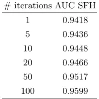
Table 1: Performance for the financial dataset with 31 covariates and 700 training records and 19 300 testing records.
# iterations AUC SFH
1 0.9418
5 0.9436
10 0.9448
20 0.9466
50 0.9517
100 0.9599
requires multiple iterations. We will therefore restrict our experiments to one single iteration.
4
Results
4.1 Accuracy of the SFH method
Table 2 shows the confusion matrix of a general binary classifier. From the
Table 2: Comparing actual and predicted classes
actual class
-1 1
predicted -1 true negative (TN) false negative (FN)
class 1 false positive (FP) true positive (TP)
confusion matrix, we can compute the true positive rate (TPR) and the false positive rate (FPR) which are given by
TPR = #TP
#TP + #FN and FPR =
#FP
#FP + #TN. (5)
By computing the TPR and FPR for varying thresholds 0≤τ≤1, we can con-struct the receiver operating characteristic curve or ROC-curve. The ROC-curve is constructed by plotting the (FPR,TPR) pairs for each possible value of the thresholdτ. In the ideal situation there would exists a point with (FPR,TPR) = (0,1), which would imply that there exists a threshold for which the model clas-sifies all test data correctly.
data and later on encrypted data. For well chosen system parameters, there will be no difference between accuracy for unencrypted vs. encrypted data since all computations on encrypted data are exact.
The first step is performed by comparing our SFH method with the standard logistic regression functionality of Matlab. This is done by applying our method with all its approximations to the plaintext data and comparing the result to the result of the “glmfit” function in Matlab. The function b = glmfit(X, y,distr) returns a vector b of coefficient estimates for a generalized linear model of the responses y on the predictors in X, using distribution distr. Generalized linear models unify various statistical models, such as linear regression, logistic regres-sion and Poisson regresregres-sion, by allowing the linear model to be related to the response variable via a link function. We use the “binomial” distribution, which corresponds to the “logit” link function andya binary vector indicating success or failure to compute the parameters of the logistic regression model with “glm-fit”.
0 0.2 0.4 0.6 0.8 1
0 0.2 0.4 0.6 0.8 1
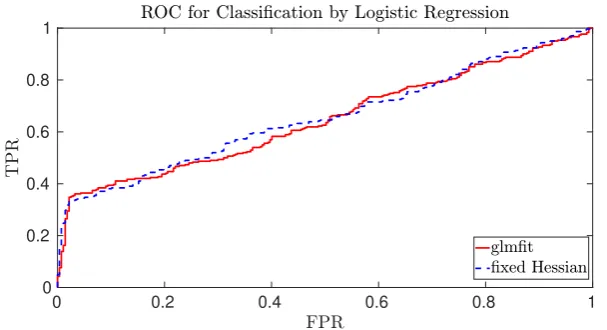
Fig. 1: ROC curve for the cancer detection scenario of iDASH with 1000 training records and 581 testing records, all with 20 covariates.
0 0.2 0.4 0.6 0.8 1 0
0.2 0.4 0.6 0.8 1
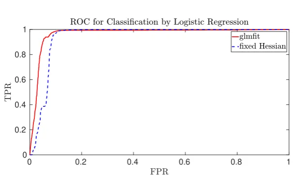
Fig. 2: ROC curve for the financial fraud detection with 1000 training records and 19 000 testing records, all with 31 covariates.
be to end up with a true positive rate of 1 and false positive rate of 0, we see from Figure 1 that for the genomics dataset both models are performing rather poorly. The financial fraud use case is, however, much more amenable to binary classification as shown in Figure 2. The main conclusion is that our SFH method performs almost as well as standard methods such as those provided by Matlab.
4.2 Implementation details and performance
Our implementation uses the FV-NFLlib software library [Cry16] which imple-ments the FV homomorphic encryption scheme. The system parameters need to be selected taking into account the following three constraints:
1. the security of the somewhat homomorphic FV scheme, 2. the correctness of the somewhat homomorphic FV scheme, 3. the correctness of the w-NIBNAF encoding.
The security of a given set of system parameters can be estimated using the work of Albrecht, Player and Scott [APS15] and the open source learning with error (LWE) hardness estimator implemented by Albrecht [Alb04]. This program esti-mates the security of the LWE problem based on the following three parameters: the degree D of the polynomial ring, the ciphertext modulusq and α=
√ 2πσ
q whereσis the standard deviation of the error distributionχerr. The security es-timation is based on the best known attacks for the learning with error problem. Our system parameters are chosen to be q= 2186, D = 4096 and σ= 20 (and thusα=
√ 2πσ
q ) which results in a security of 78 bits.
this noise under the correctness bound and in particular, we obtain an upper boundtmaxof the plaintext modulus. Similarly, to ensure correct decoding, the coefficients of the polynomial encoding the result must remain smaller than the size of the plaintext modulus t. This condition results in a lower bound on the plaintext modulus tmin.
It turns out that these bounds are incompatible for the chosen parameters, so we have to rely on the Chinese Remainder Theorem to decompose the plaintext space into smaller parts that can be handled correctly. The plaintext modulus
t is chosen as a product of small prime numbers t1, t2, . . . , tn with ∀i ∈ {1, . . . , n} : ti ≤tmax and t =Q
n
i=1 ti ≥tmin, where tmax is determined by the correctness of the FV scheme andtminby the correctness of thew-NIBNAF decoding. The CRT then gives the following ring isomorphism:
Rt→Rt1×. . .×Rtn:g(X)7→(g(X) modt1, . . . , g(X) modtn). and instead of performing the training algorithm directly over Rt, we compute with each of the Rti’s by reducing the w-NIBNAF encodings modulo ti. The resulting choices for the plaintext spaces are given in Table 3.
Table 3: The parameters defining plaintext encoding
w t
genomic data (1) 71 5179·5189·5197
financial data (2) 150 2237·2239
Since we are using the Chinese Remainder Theorem, each record will be encrypted using two (for the financial fraud case) or three (for the genomics case) ciphertexts. As such, a time-memory trade off is possible depending on the requirements of the application. One can choose to save computing time by executing the algorithm for the different ciphertexts in parallel; or one can choose to save memory by computing the result for each plaintext space Rti consecutively and overwriting the intermediate values of the computations in the process.
The memory required for each ciphertext is easy to estimate: a ciphertext consists of 2 polynomials ofRq =Zq[X]/(XD+1), so its size is given by 2Dlog2q which is≈186kB for the chosen parameter set. Due to the use of the CRT, we require T (with T = 2 or T = 3) ciphertexts to encrypt each record, so the general formula for the encrypted dataset size is given by:
T(d+ 1)N2Dlog2q bits,
with T the number of prime factors used to split the plaintext modulus t and
Table 4: Performance for the genomic dataset with a fixed number of covariates equal to 20. The number of testing records is for each row equal to the total number of input records (1581) minus the number of training records.
# training records computation time AUC SFH AUC glmfit
500 22 min 0.6348 0.6287
600 26 min 0.6298 0.6362
800 35 min 0.6452 0.6360
1000 44 min 0.6561 0.6446
Table 5: Performance for the genomic dataset with a fixed number of training records equal to 500 and the number of testing records equal to 1081.
# covariates computation time AUC SFH AUC glmfit
5 7 min 0.65 0.6324
10 12 min 0.6545 0.6131
15 17 min 0.6446 0.6241
20 22 min 0.6348 0.6272
compute the matrix ˜H by first computing ¯H and subsequently summing each row, the complexity would beO(N d2). However, the formula of thek-th diagonal element of ˜H is given by −41Pd+1
j=1 PN
i=1xk,ixj,i
, which can be rewritten as −1
4 PN
i=1xk,i P d+1 j=1xj,i
. This formula shows that it is more efficient to first sum all the rows of X and then perform a matrix vector multiplication with complexityO(N d).
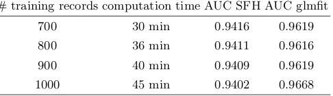
Table 6: Performance for the financial dataset with a fixed number of covariates equal to 31. The number of testing records is for each row equal to the total number of input records (20 000) minus the number of training records.
# training records computation time AUC SFH AUC glmfit
700 30 min 0.9416 0.9619
800 36 min 0.9411 0.9616
900 40 min 0.9409 0.9619
1000 45 min 0.9402 0.9668
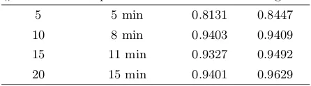
Table 7: Performance for the financial dataset with a fixed number of records equal to 500 and the number of testing records equal to 19 500.
# covariates computation time AUC SFH AUC glmfit
5 5 min 0.8131 0.8447
10 8 min 0.9403 0.9409
15 11 min 0.9327 0.9492
20 15 min 0.9401 0.9629
computations in the implementation.
In Table 4 and Table 5 we see that often the AUC value of the SFH model is slightly higher than the AUC value of the glmfit model. However, as mentioned before both models perform poorly on this dataset. Since our SFH model contains many approximations we expect it to perform slightly worse than the “glmfit” model. Only slightly worse because Figure 1 and Figure 2 already showed that the SFH models classifies the data almost as well as the “glmfit” model. This is consistent with the results for the financial dataset shown in Table 6 and Table 7, which we consider more relevant than the results of the genomic dataset due to the fact that both models perform better on this dataset.
5
Discussion
The experiments of this article show promising results for the simple iterative method we propose as an algorithm to compute the logistic regression model. A first natural question is whether this technique is generalizable to other machine learning problems. In [B¨oh92], B¨ohning describes how to adapt the lower bound method to make it applicable to multinomial logistic regression, it is likely this adaption will also apply to our SFH technique and hence our SFH technique can most likely also be applied to construct a multinomial logistic regression model. In the case of neural networks we can refer to [BCIV17]; in order to construct the neural network one needs to rank all the possibilities and only keep the best performing neurons for the next layer. Constructing this ranking homomorphi-cally is not straightforward and not considered at all in our algorithm, hence neural networks will require more complicated algorithms.
6
Conclusions
The simple, but effective, iterative method presented in this paper allows one to train a logistic regression model on homomorphically encrypted input data. Our method can be used to outsource the training phase of logistic regression to a cloud service in a privacy preserving manner. We demonstrated the performance of our logistic training algorithm on two real life applications using different numeric data types. In both cases, the accuracy of our method is only slightly worse than standard algorithms to train logistic regression models. Finally, the time complexity of our method grows linearly in the number of covariates and the number of training input data points.
References
[AHTPW16] Yoshinori Aono, Takuya Hayashi, Le Trieu Phong, and Lihua Wang. Scal-able and secure logistic regression via homomorphic encryption. In Pro-ceedings of the Sixth ACM Conference on Data and Application Security
and Privacy, CODASPY ’16, pages 142–144, New York, NY, USA, 2016.
ACM.
[Alb04] Martin Albrecht. Complexity estimates for solving LWE, 2000–2004. [APS15] Martin R. Albrecht, Rachel Player, and Sam Scott. On the concrete
hardness of learning with errors. J. Mathematical Cryptology, 9(3):169– 203, 2015.
[BBB+17] Charlotte Bonte, Carl Bootland, Joppe W. Bos, Wouter Castryck, Ilia Iliashenko, and Frederik Vercauteren. Faster homomorphic function eval-uation using non-integral base encoding. In Wieland Fischer and Naofumi Homma, editors,Cryptographic Hardware and Embedded Systems – CHES 2017, pages 579–600, Cham, 2017. Springer International Publishing. [BCIV17] Joppe W. Bos, Wouter Castryck, Ilia Iliashenko, and Frederik
Ver-cauteren. Privacy-friendly forecasting for the smart grid using homomor-phic encryption and the group method of data handling. In Marc Joye and Abderrahmane Nitaj, editors,Progress in Cryptology - AFRICACRYPT 2017, pages 184–201, Cham, 2017. Springer International Publishing. [BEHZ16] Jean-Claude Bajard, Julien Eynard, Anwar Hasan, and Vincent Zucca.
A full rns variant of fv like somewhat homomorphic encryption schemes.
IACR Cryptology ePrint Archive, 2017:22, 2016.
[BL88] Dankmar B¨ohning and Bruce G Lindsay. Monotonicity of quadratic-approximation algorithms. Annals of the Institute of Statistical
Mathe-matics, 40(4):641–663, 1988.
[BLN14] Joppe W Bos, Kristin Lauter, and Michael Naehrig. Private predictive analysis on encrypted medical data. Journal of biomedical informatics, 50:234–243, 2014.
[B¨oh92] Dankmar B¨ohning. Multinomial logistic regression algorithm. Annals of
the Institute of Statistical Mathematics, 44(1):197–200, 1992.
[CIV17] Wouter Castryck, Ilia Iliashenko, and Frederik Vercauteren. Homomor-phic sim2d operations: Single instruction much more data. IACR
Cryp-tology ePrint Archive, 2017:22, 2017.
[FV12] Junfeng Fan and Frederik Vercauteren. Somewhat practical fully homo-morphic encryption. IACR Cryptology ePrint Archive, 2012:144, 2012. [Ger31] Semyon Aranovich Gershgorin. Uber die abgrenzung der eigenwerte einer
matrix. Bulletin de l’Acad´emie des Sciences de l’URSS. Classe des
sci-ences math´ematiques et na, (6):749–754, 1931.
[KSW+18] Miran Kim, Yongsoo Song, Shuang Wang, Yuhou Xia, and Xiaoqian Jiang. Secure logistic regression based on homomorphic encryption.IACR
Cryptology ePrint Archive, 2018:14, 2018.
[LPR13] Vadim Lyubashevsky, Chris Peikert, and Oded Regev. On Ideal Lattices and Learning with Errors over Rings. J. ACM, 60(6):Art. 43, 35, 2013. [NLV11] Michael Naehrig, Kristin Lauter, and Vinod Vaikuntanathan. Can
homo-morphic encryption be practical? InProceedings of the 3rd ACM
Work-shop on Cloud Computing Security WorkWork-shop, CCSW ’11, pages 113–124,
New York, NY, USA, 2011. ACM.