Data
Angela J¨aschke1 and Frederik Armknecht1
University of Mannheim, Germany
Abstract. In the context of Fully Homomorphic Encryption, which al-lows computations on encrypted data, Machine Learning has been one of the most popular applications in the recent past. All of these works, however, have focused on supervised learning, where there is a labeled training set that is used to configure the model. In this work, we take the first step into the realm of unsupervised learning, which is an important area in Machine Learning and has many real-world applications, by ad-dressing the clustering problem. To this end, we show how to implement theK-Means-Algorithm. This algorithm poses several challenges in the FHE context, including a division, which we tackle by using a natural encoding that allows division and may be of independent interest. While this theoretically solves the problem, performance in practice is not op-timal, so we then propose some changes to the clustering algorithm to make it executable under more conventional encodings. We show that our new algorithm achieves a clustering accuracy comparable to the original
K-Means-Algorithm, but has less than 5% of its runtime.
Keywords: Machine Learning, Clustering, Fully Homomorphic Encryption
1
Introduction
1.1 Motivation
Fully Homomorphic Encryption (FHE) schemes can in theory perform arbitrary computations on encrypted data. Since the discovery of FHE, many applica-tions have been proposed, ranging from medical over financial to advertising scenarios. The underlying idea is mostly the same: Suppose Alice has some con-fidential data X which she would like to utilize, and Bob has an algorithm A which he could apply to Alice’s data for money. However, conventionally, either Alice would have to give her confidential data to Bob, or run the algorithm her-self, for which she may not have the know-how or computational power. FHE allows Alice to encrypt her data to C := Enc(X) and send it to Bob. Bob can convert his algorithm Ainto a functionA0 over the ciphertext space and apply
it to the encrypted data, resulting in R:=A0(C). He can then send this result
whole time, Bob learns nothing about the data entries. Note that the function-ality where Bob’s algorithm is also kept secret from Alice is not traditionally guaranteed by FHE, but can in practice be achieved via a property calledcircuit privacy, in the sense that Alice learns nothing except the resultA(X).
One of the most popular applications of FHE has been Machine Learning, with many works focusing on Neural Networks and different variants of regression (see Related Work in Section 2). To our knowledge, all works in this line are concerned withsupervised learning. This means that there is a training set with known outcomes, and the algorithm tries to build a model that matches the desired outputs to the inputs as well as possible. When the training phase is done, the algorithm can be applied to new instances to predict unknown outcomes.
However, there is a second branch in Machine Learning that has not been touched by FHE research:Unsupervised learning. For these kinds of algorithms, there are no labeled training examples, there is simply a dataset on which some kind of analysis shall be performed. An example of this is clustering, where the aim is to group data entries that are similar in some way. The number of clusters might be a parameter that the user enters, or it may be automatically selected by the algorithm. Clustering has numerous applications like genome sequence analysis, market research, medical imaging or social network analysis, to name a few, some of which inherently involve sensitive data – making a privacy-preserving evaluation with FHE even more interesting.
1.2 Contribution
In this work, we approach this unexplored branch of Machine Learning and show how to implement the K-Means-Algorithm, an important clustering algorithm, on encrypted data. We discuss the problems that arise when trying to evaluate theK-Means-Algorithm on encrypted data, and show how to solve them. To this end, we first present a natural encoding that allows the execution of the algorithm as it is (including the usually challenging division by an encrypted value), but is not optimal in terms of performance. We then present a modification to theK -Means-Algorithm that performs comparably in terms of clustering accuracy, but is much more FHE-friendly in that it avoids division by an encrypted value. We include another modification that trades accuracy for efficiency in the involved comparison operation, and compare the runtimes of these approaches.
2
Related Work
Machine Learning as an application of FHE was first proposed in [35], and subsequently there have been numerous works on the subject, to our knowledge all concerned with supervised learning. The most popular of these applications seem to be (Deep) Neural Networks (see [26], [21], [10], [36], and [7]) and (Linear) Regression (e.g., [32], [17], [4] or [22]), though there is also some work on other algorithm classes like decision trees and random forests ([41]), or logistic regres-sion ([6],[30],[29] and [5]). In contrast, our work is concerned with the clustering problem from unsupervised Machine Learning.
The K-Means-Algorithm has been a subject of interest in the context of privacy-preserving computations for some time, but to our knowledge all pre-vious works like [9], [25], [24], [31] and [42] require interaction between several parties, e.g. via Multiparty Computation (MPC). For a more comprehensive overview of theK-Means-Algorithm in the context of MPC, we refer the reader to [34]. While this interactivity may certainly be a feasible requirement in many situations, and indeed MPC is likely to be faster than FHE in these cases, we feel that there are several reasons why a non-interactive solution as we present it is an important contribution.
1. Client Economics: In MPC, the computation is split between different parties, each performing some computations in each round and combining the results. In FHE computations, the entire computation is performed by the service provider – even if this computation on encrypted data is more ex-pensive than the total MPC computation, the client reduces his effort to zero this way, making this solution more attractive to him and thus generating a demand for it.
2. Function Privacy: To see this, imagine the K-Means-Algorithm in this paper as a placeholder for a more complex proprietary algorithm that the service provider executes on the client’s data as a service. This algorithm could utilize building blocks from theK-Means-Algorithm that we present in this paper, or involve theK-Means-Algorithm as a whole in the context of pipelining several algorithms together, or be something completely new. In this case, the service provider would want to prevent the user from learning the details of this algorithm, as it is his business secret. While FHE per se does not guarantee this functionality, all schemes today fulfill the require-ment ofcircuit privacyneeded to achieve it. Thus it seems that for this case, FHE would be the preferred solution.
3. Future Efficiency Gain: The field of MPC is much older than that of FHE, and efficiency for the latter has increased by a factor of 104 in the
last six years alone. To argue that MPC is faster and thus FHE solutions are superfluous seems premature at this point, and our contributions are not specific to any one implementation, but work on all FHE schemes that support a{0,1} plaintext space.
● ●● ● ● ● ● ● ● ● ● ● ● ● ● ● ● ● ● ● ● ● ● ● ● ● ● ● ● ● ● ● ● ● ● ● ●● ● ● ● ●●● ● ● ● ● ● ● ● ● ● ● ● ● ● ● ● ● ● ● ● ●● ● ● ● ●● ● ● ● ● ● ● ● ● ● ●● ● ● ● ● ● ● ● ● ● ● ● ● ● ● ● ● ● ● ● ● ● ● ● ● ● ● ● ● ● ●● ●● ● ● ● ● ● ● ● ● ● ● ● ● ●●● ● ● ● ● ● ● ● ● ● ● ● ● ● ●● ● ● ● ● ● ● ● ●● ● ● ● ● ● ● ●● ● ● ● ● ● ● ● ● ● ● ● ● ● ● ● ● ●● ● ● ● ● ● ● ● ● ● ●● ● ● ● ● ● ● ● ● ● ● ●● ●●●● ● ●● ● ● ● ● ● ● ● ●● ● ● ● ● ● ● ● ● ● ● ● ● ● ● ● ● ● ● ● ● ● ● ● ● ● ● ● ● ● ● ● ● ● ● ● ● ● ● ● ● ● ● ●● ● ● ● ● ● ● ● ● ●● ● ● ●● ● ●● ●● ● ● ● ● ● ● ● ● ● ● ● ● ● ● ● ● ● ● ● ● ● ● ● ● ● ● ● ● ● ● ● ● ● ● ● ●●● ● ● ● ● ● ● ● ● ● ● ● ● ● ● ● ● ● ● ● ● ● ● ● ● ● ● ● ● ● ● ● ● ● ●● ● ● ● ● ● ● ● ● ● ● ● ● ● ● ● ● ● ● ● ● ● ● ● ● ● ● ● ● ● ● ● ● ● ● ● ● ● ● ● ● ● ● ● ● ● ●
0 5 10 15 20
0
5
10
15
20
Data and initial centroids
x
y
0 5 10 15 20
0 5 10 15 20 First assignment x y
0 5 10 15 20
0
5
10
15
20
First centroid movement
x
y
0 5 10 15 20
0 5 10 15 20 Second assignment x y
0 5 10 15 20
0
5
10
15
20
Second centroid movement
x
y
0 5 10 15 20
0 5 10 15 20 Third assignment x y
0 5 10 15 20
0
5
10
15
20
Third centroid movement
y
0 5 10 15 20
0 5 10 15 20 Final assignment y
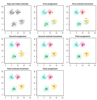
Fig. 1.An illustration of theK-Means-Algorithm.
3
Preliminaries
In this section, we cover underlying concepts like the K-Means-Algorithm, en-coding issues, our choice of implementation library, and the datasets we use.
3.1 The K-Means Algorithm
TheK-Means-Algorithm is one of the most well-known clustering algorithms in unsupervised learning. Published in [33], it is considered an important bench-mark algorithm and is frequently the subject of current research to this day.
nearest regarding Euclidean distance, and assigns the data entry to that centroid. When this has been done for all data entries, the second step begins: During the
Move Centroidsstep, the cluster centroids are moved by setting each centroid as the average of all data entries that were assigned to it in the previous step. These two steps are repeated for a set number of timesTor until the centroids do not change anymore. We use the first method. A visualization of theK -Means-Algorithm can be seen in Figure 1.
The exact workings of theK-Means-Algorithm are presented in Algorithm 1, where operations like addition and division are performed component-wise if applied to vectors.
Algorithm 1:TheK-Means-Algorithm
Input:Data setX={x1, . . . , xm}//xi∈R` for some ` Input:Number of clustersK
Input:Number of iterationsT
// Initialization
1 Randomly reorderX;
2 Set centroidsck=xkfork= 1 toK;
// Keep track of centroid assignments
3 Generatem-dimensional vectorA;
// Keep track of denominators in average computation
4 GenerateK-dimensional vectord= (d1, . . . , dK);
5 forj= 1toT do
// Cluster Assignment
6 fori= 1tomdo
7 ∆=∞;
8 fork= 1toKdo
9 ∆˜:=||xi−ck||2;
// Check if current cluster is closer than previous closest
10 if∆ < ∆˜ then
// If so, update∆ and assign data entry to current cluster
11 ∆= ˜∆;
12 Ai=k;
13 end
14 end
15 end
// Move Centroids
16 fork= 1toKdo
17 ck= 0;
18 dk= 0;
19 end
20 fori= 1tomdo
// Add the data entry to its assigned centroid
21 c
Ai+=xi;
// Increase the appropriate denominator
22 dAi+= 1
23 end
24 fork= 1toKdo
// Divide centroid by number of assigned data entries to get average
25 ck=ck/dk;
26 end
27 end
The output of the algorithm is the values of the centroids, or the cluster assignment for the data entries (which can easily be computed from the former). We opt for the first approach. Accuracy can either be measured in terms of correctly classified data entries, which assumes that the correct classification is known (there might not even exist a unique best solution), or via the so-called cost function, which measures the (average) distance of the data entries to their assigned cluster centroids. We opt for the first approach because our datasets are benchmarking sets for which the labels are indeed provided, and it allows better comparability between the different algorithms. To aid the reader, we present a brief recap of the variables that we use:
– K: Number of clusters. – ck: Cluster centroid k. – m: Number of data points. – X={x1, . . . , xm}: The dataset. – `: The dimension of the data.
– dk: Denominator of centroidkin the average computation (i.e., the number of data entries assigned to that cluster).
– T: Number of rounds to run the algorithm. – ∆: A number to hold distances (later: a vector).
– A: The cluster assignment vector (m-dimensional), later a boolean matrix (m×K).
3.2 Encoding
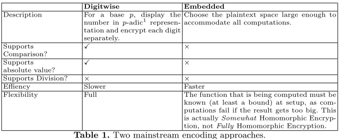
FHE schemes generally have finite fields as a plaintext space, and any rational numbers (which can be scaled to integers) must be embedded into this plaintext space. There are two main approaches in literature, which we quickly compare side by side in Table 1. Note that for absolute value computation and comparison, we need to use the digitwise encoding.
Digitwise Embedded
Description For a base p, display the
number inp-adic1
represen-tation and encrypt each digit separately.
Choose the plaintext space large enough to accommodate all computations.
Supports Comparison?
X ×
Supports
absolute value? X
×
Supports Division? × ×
Effiency Slower Faster
Flexibility Full The function that is being computed must be
known (at least a bound) at setup, as com-putations fail if the result gets too big. This
is actuallySomewhatHomomorphic
Encryp-tion, notFullyHomomorphic Encryption.
Table 1.Two mainstream encoding approaches.
1
3.3 FHE Library Choice
In [27], it was shown that among all bases p for digitwise p-adic encoding in FHE computations, the choicep= 2 is best in terms of the number of additions and multiplications to be performed on the ciphertexts. Hence, we use an FHE scheme with a plaintext space of {0,1}. The currently fastest FHE implemen-tation TFHE ([38]), which works on this plaintext space {0,1}, states “Since the running time per gate seems to be the bottleneck of fully homomorphic en-cryption, an optimal circuit for TFHE is most likely a circuit with the smallest possible number of gates, and to a lesser extent, the possibility to evaluate them in parallel.”. Thus, this library is a perfect choice for us, and we will use the binary encoding for signed integers and tweaks presented in [26] for maximum efficiency. Our code for the implementations of all presented algorithms using the TFHE library is available upon request.
3.4 Datasets
To evaluate performance, we use four datasets from the FCPS dataset [39] to monitor performance:
– The Hepta dataset consists of 212 data points of 3 dimensions. There are 7 clearly defined clusters.
– The Lsun dataset is 2-dimensional with 400 entries and 3 classes. The clusters have different variances and sizes.
– The Tetra dataset is comprised of 400 entries in 3 dimensions. There are 4 clusters, which almost touch.
– The Wingnut dataset has only 2 clusters, which are side-by-side rectangles in 2-dimensional space. There are 1016 entries.
For accuracy measurements, each version of the algorithm was run 1000 times for number of iterations T = 5,10, ...,45,50 on each dataset. For runtimes on encrypted data, we used the Lsun dataset.
4
Approach 1: Implementing the Exact
K
-Means-Algorithm
4.1 FHE Challenges
Fully homomorphic encryption schemes can easily compute additions and mul-tiplications on the underlying plaintext space, and most also offer subtraction. Using these operations as building blocks, more complex functionalities can be obtained. However, there are three elements in the K-Means-Algorithm that pose challenges, as it is not immediately clear how to obtain them from these building blocks. We list these (with the line numbers referring to the pseudocode of Algorithm 1) and quickly explain how we solve them.
– The distance metric (Line 9,∆(x, y) =||x−y||2:=pPi(xi−yi)2): To our knowledge, taking the square root of encrypted data has not been imple-mented yet. In Section 4.2, we will argue that the Euclidean norm is an arbi-trary choice in this context and solve this problem by using theL1-distance
∆(x, y) =||x−y||1:=Pi(|xi−yi|) instead of the Euclidean distance. – Comparison (Line 10, ˜∆ < ∆) in finding the centroid with the smallest
distance to the data entry: This has been constructed from bit multiplications and additions in [26] for bitwise encoding, so we view this issue as solved. A more detailed explanation can be found in Appendix A.2.
– Division (Line 25,ck =ck/dk) in computing the new centroid value as the average of the assigned data points: In FHE computations, division by an encrypted value is usually not possible (whereas division by an unencrypted value is no problem). We present a way of implementing the division with a new encoding in Section 4.3, and propose a modified version of the Algorithm in Section 5 that only needs division by a constant.
4.2 The Distance Metric
Traditionally, the distance measure used with the K-Means Algorithm is the Euclidean Distance ∆(x, y) = ||x−y||2 :=pPi(xi−yi)2, also known as the
L2-Norm, as it is analytically smooth and thus reasonably well-behaved.
How-ever, in the context of K-Means Clustering, smoothness is irrelevant, and we may look to other distance metrics. Concretely, we consider theL1-Norm2(also
known as the Manhattan-Metric)∆(x, y) := P
i(|xi−yi|). This has a consid-erable advantage over the Euclidean distance: Firstly, we do not need to take a square root, which to our knowledge has not yet been achieved on encrypted data. Secondly, of course one could apply the standard trick and not take the root, working instead with the sum of squared distances – however, this would mean a considerable efficiency loss. To see this, first note that multiplying two numbers takes significantly longer than taking the absolute value. Also, recall that multiplying two numbers of equal bitlength results in a number of twice that bitlength. These much longer numbers then have to be summed up, and al-ready the summation step is a bottleneck of the whole computation on encrypted data even when working with short numbers in theL1 norm. The result of the
2
[1] in fact argues that for high-dimensional spaces, theL1-Norm is more meaningful
summation is an input to the algorithm that finds the minimum (Algorithm 3 on page 15), which also takes a significant amount of time and would likely more than double in runtime if the input length doubled.
Taking the absolute value can easily be achieved through a digit-wise encod-ing like the binary encodencod-ing which we use: We can use the MSB as the conditional (it is 1 if the number is negative and 0 if it is positive) and use a multiplexer3
gate applied to the value and its negative. The concrete algorithm can be seen in Algorithm 5 in Appendix A.1. Thus, using theL1-Norm is not only justified
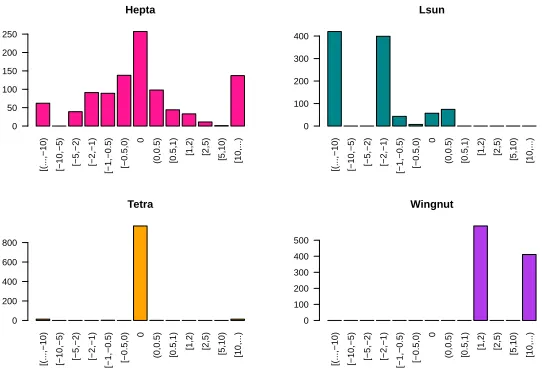
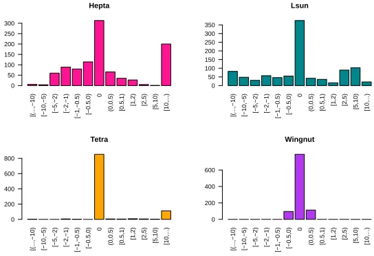
by the arbitrariness of the Euclidean Norm, but is also much more efficient. We compare the clustering accuracy in Figure 2.
[(...,−10) [−10,−5) [−5,−2) [−2,−1) [−1,−0.5) [−0.5,0)
0
(0,0.5) [0.5,1) [1,2) [2,5) [5,10) [10,...)
Hepta
0 50 100 150 200 250
[(...,−10) [−10,−5) [−5,−2) [−2,−1) [−1,−0.5) [−0.5,0)
0
(0,0.5) [0.5,1) [1,2) [2,5) [5,10) [10,...)
Lsun
0 100 200 300 400
[(...,−10) [−10,−5) [−5,−2) [−2,−1) [−1,−0.5) [−0.5,0)
0
(0,0.5) [0.5,1) [1,2) [2,5) [5,10) [10,...)
Tetra
0 200 400 600 800
[(...,−10) [−10,−5) [−5,−2) [−2,−1) [−1,−0.5) [−0.5,0)
0
(0,0.5) [0.5,1) [1,2) [2,5) [5,10) [10,...)
Wingnut
0 100 200 300 400 500
Fig. 2.Difference in percent of data points mislabeled forL1-norm compared to the L2-norm (% mislabeledL1)-(% mislabeledL2)
.
For both versions of the distance metric, we calculated the percentage of wrongly labeled data points for 1000 runs, which we can do because the datasets we use come with the correct labels. We then plotted histograms of the difference (in percent mislabeled) between the L1-norm and the L2-norm for each run.
Thus, a value of 0.5 means that theL1 norm version misclassified 0.5% more
data entries than theL2-version, and−2 means that theL1version misclassified
2% less data entries than theL2-version. Each subplot corresponds to one of the
four datasets we used.
We see that indeed, it is impossible to say which metric is better – for the Hepta dataset, the performance is very balanced, for the Lsun dataset, theL1
-3
MUX(c, a, b) = (
a, c= 1
norm performs much better, for the Tetra dataset, they nearly always perform exactly the same, and for the Wingnut dataset, the L2-norm is consistently
better.
4.3 Fractional Encoding
Suppose we have routines to perform addition, multiplication and comparison on numbers that are encoded bitwise – we denote these routines withAdd(a, b),
Mult(a, b) and Comp(a, b), where the latter returns 1 (encrypted) ifa < band 0 otherwise. The idea is to express the number we wish to encode as a fraction and encode the numerator and denominator separately. Concretely, to encode a number a, we choose the denominator ad randomly in a certain range (like
ad∈[2k,2k+1) for somek) and compute the nominatoran asan=ba·ade. We then encode both separately, so we havea= (an, ad).
If we then want to perform computations (including division) on values en-coded in this way, we can express the operations using the subroutines from the binary encoding through the regular computation rules for fractions:
– a+b:FracAdd((an, ad),(bn, bd))
= Add(Mult(an, bd),Mult(ad, bn)),Mult(ad, bd)
– a·b:FracMult((an, ad),(bn, bd)) = Mult(an, bn),Mult(ad, bd)
– a/b:FracDiv((an, ad),(bn, bd)) = Mult(an, bd),Mult(ad, bn)
– a≤b:FracComp((an, ad),(bn, bd)) :
This is slightly more involved. Note that the MSB determines the sign of the number (1 if it is negative and 0 otherwise). Let
c:= Sign(ad)⊕Sign(bd), and let
MUX(c, a, b) =
(
a, c= 1
b, c= 0 be the multiplexer gate.
Then we set
d:=MUX(c,Mult(an, bd),Mult(ad, bn)) and
e:=MUX(c,Mult(ad, bn),Mult(an, bd)) and output the result asComp(e, d).
To make this comparison operation clearer, consider the following: We basi-cally want to compare an
ad and
bn
bd, so we instead ask whether
an·bd≤bn·ad.
However, if the sign of exactly one of the denominators is negative, this changes the direction of the inequality operator, so that we would need to compute
instead. Thus, we assign the values conditionally through the multiplexer gate before comparing them: If theXORof the sign bits is 0, we compare
(e:=an·bd)≤(d:=bn·ad),
and if it is 1, i.e., exactly one of the denominators is negative, we compare (e:=bn·ad)≤(d:=an·bd).
Controlling the Bitlength Notice that every single one of these operations requires a multiplication of some sort, which means that the bitlengths of the nominators and denominators doubles with each operation, as there is no can-cellation when the data is encrypted. However, note that in bitwise encoding, deleting the lastk least significant bits corresponds to dividing by 2k and trun-cating. Doing this for both nominator and denominator yields roughly the same result as before, but with lower bitlengths. As an example, suppose that we have encoded our integers with 15 bits, and after multiplication we thus have 30 bits in nominator and denominator, e.g. 651049779/1053588274≈0.617936. Then dividing both nominator and denominator by 215 and truncating yields
19868/32152, which evaluates to 0.617939≈0.617936. The accuracy can be set through the original encoding bitlength (15 here).
4.4 Evaluation
While this new encoding theoretically allows us to perform theK-Means-Algorithm and solves the division problem in FHE, we now discuss the practical perfor-mance in terms of accuracy and runtime.
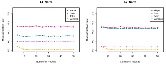
Accuracy To see how the exact algorithm performs, we use the four datasets from Section 3.4. We ran the exact algorithm 1000 times for number of itera-tionsT= 5,10, ...,45,50, and for sake of completeness we include both distance metrics. The results in this section were obtained by running the algorithms in unencrypted form. We first examine the effect ofT on the exact version of the algorithm by looking at the average (over the 1000 runs) misclassification rate for both metrics. The result can be seen in Figure 3.
We can see that the rate levels off after about 15 rounds in all cases, so there is no reason to iterate further.
10 20 30 40 50
0.0
0.1
0.2
0.3
0.4
L1−Norm
Number of Rounds
Misclassification Rate
●
● ● ● ●
● ● ● ● ● ●
Hepta Lsun Tetra Wingnut
10 20 30 40 50
0.0
0.1
0.2
0.3
0.4
L2−Norm
Number of Rounds
Misclassification Rate
●
● ● ● ● ● ● ● ● ● ●
Hepta Lsun Tetra Wingnut
Fig. 3.Misclassification rate with increasing rounds for exact algorithms.
end with a 0 in the denominator. Both these cases result in completely arbitrary and unusable results. The reason why it is so hard to set the shortening parameter properly is that generally, nominator and denominator will not require the same number of bits. Concretely, this will only be the case when the value of the number being in encoded is in the interval (1/2,2), and even so, this interval is not closed under addition or multiplication, so this problem can arise even if plaintexts are scaled into this interval.
The problem is that because the data is encrypted, we cannot see the actual size of the underlying data, so the shortening parameter cannot be set dynam-ically – in fact, if it were possible to set it dynamdynam-ically, this would imply that the FHE scheme is insecure. Also, even setting the parameter roughly requires extensive knowledge about the encrypted data, which the data owner may not want to share with the computing party.
Runtime The second issue with this encoding is the runtime. Even though TFHE is the most efficient FHE library with which many computational tasks approach practically feasible runtimes, the fact that this encoding requires sev-eral multiplications on binary numbers for each elementary operation slows it down considerably. We compare the runtimes of all our algorithms in Section 7, and as we will see, running theK-Means-Algorithm on a real-world dataset with this Fractional Encoding would take almost 1.5 years on our computer.
4.5 Conclusion
5
Approach 2: The Stabilized
K
-Means-Algorithm
In this section, we present a modification of theK-Means algorithm that avoids the division in the MoveCentroid-step. Concretely, recall that conventional en-codings in FHE, like the binary one we will use, do not allow the computation of
c1/c2 wherec1 andc2 are ciphertexts, but it is possible to computec1/a where
a is some unencrypted number. Our algorithm uses this fact to exchange the ciphertext division in Line 25 of Algorithm 1 (page 5) for a constant division, resulting in a variant that can be computed with more established and efficient encodings than the one from Section 4.3. Note that this approach of approxi-mating or replacing a function that is hard to compute on encrypted data is not unusual in the FHE context – for example, [21] does this for several different functions in building a neural network on encrypted data.
We present this new algorithm in Section 5.2, and compare the accuracy of the returned results to the originalK-Means-Algorithm in Section 5.3.
5.1 Encoding
The dataset we use to evaluate our algorithms consists of rational numbers. To encode these so that we can encrypt them bit by bit, we scaled them with a fac-tor of 220and truncated to obtain an integer. We then used Two’s Complement
encoding to accommodate signed numbers, and switched to Sign-Magnitude En-coding for multiplication. Note that deleting the last 20 bits corresponds to dividing the number by 220 and truncating, so the scaling factor can remain
constant even after multiplication, where it would normally square.
5.2 The Algorithm
Recall that in the originalK-Means-Algorithm, theMoveCentroid-step consists of computing each centroid as the average of all data entries that have been assigned to it. More specifically, suppose that we have a (m×K)-dimensional cluster assignment matrixA, where
Aik=
(
1, Data entryxi is assigned to centroid ck 0 else.
Then computing the new centroid valueck consists of multiplying the data en-tries xi with the corresponding entry Aik and summing up the results before dividing by the sum over the respective columnk ofA:
ck = m
X
i=1
xi·Aik
m
X
i=1
Aik.
Algorithm 2:The StabilizedK-Means-Algorithm Input:Data setX={x1, . . . , xm}//xi∈R` for some ` Input:Number of clustersK
Input:Number of iterationsT
// Initialization
1 Randomly reorderX;
2 Set centroidsck=xkfork= 1 toK;
// Keep track of centroid assignments
3 Generate (m×K)-dimensional boolean matrixAset to 0;
4 forj= 1toT do
// Cluster Assignment
5 fori= 1tomdo
6 ∆=∞;
7 fork= 1toKdo
// Compute distances to all centroids
8 ∆k:=||xi−ck||1;
9 end
// Theith row of A has all0’s except at the column corresponding to the
centroid with the minimum distance
10 A[i,·]←FindMin(∆1, . . . , ∆K);
11 end
// Move Centroids
12 fork= 1toKdo
// Keep old centroid value
13 c¯k=ck;
14 ck= 0;
15 fori= 1tomdo
// IfAik== 1, addxi to ck, otherwise addc¯k to ck
16 ck+=MUX(Aik, xi,c¯k);
17 end
// Divide by number of termsm
18 ck=ck/m
19 end
20 end
Output:{c1, . . . , cK}
easily done with a multiplexer gate (or more specifically, by abuse of notation, a multiplexer gate applied to each bit of the two inputs) with the entryAik as the conditional boolean variable:
ck= m
X
i=1
MUX(Aik, xi,c¯k)
m.
The sum now always consists of m terms, so we can divide by the unen-crypted constant m. It is also now obvious why we call it the stabilized K -Means-Algorithm: We expect the centroids to move much more slowly, because the old centroid values stabilize the value in the computation (more so with fewer data entries that are assigned to a centroid). The details of this new algo-rithm can be found in Algoalgo-rithm 2, with the changes compared to the original
K-Means-Algorithm shaded.
Algorithm 3:FindMin(∆1, . . . , ∆K)
Input:Distances∆1, . . . , ∆Kof current data entryito all centroidsc1. . . , cK
Input:Rowiof Cluster Assignment matrixA, denotedA[i,·]
// Set all entries0 except the first
1 SetA[i,·] = [1,0, . . . ,0];
// Set the minimum to∆1
2 Setminval=∆1;
3 fork= 2toKdo
//C is a Boolean value,C= 1iff minval≤∆k
4 C=Compare(minval, ∆k);
5 forr= 1tok−1do
// Set all previous values to0 if new min is ∆k, don’t change if new min is
old min 6 A[i, r] =A[i, r]·C;
7 end
// SetA[i, k] to 1if ∆k is new min, 0otherwise
8 A[i, k] =¬C;
9 ifk6=Kthen
// Update the minval variable unless we’re done
10 minval=MUX(C,minval, ∆k);
11 end
12 end
Output:A[i,·]
with a new functionFindMin(∆1, . . . , ∆K) due the change in data structure of
A (from an integer vector to a boolean matrix) and for readability. This new function outputs
A[i,·]←FindMin(∆1, . . . , ∆K)
such that theithrow ofA,A[i,·], has all 0’s except at the column corresponding to the centroid with the minimum distance toxi. The idea is to run theCompare
circuit to obtain a Boolean value:
Compare(x, y) =
(
1, x < y,
0, x≥y.
We start by comparing the first two distances∆1and∆2and setting the Boolean
value asC:=Compare(∆1, ∆2). Then we can writeA[i,1] =CandA[i,2] =¬C
and keep track of the current minimum throughminval:=MUX(C, ∆1, ∆2). We
then compareminval to∆3etc. until we have reached ∆K. Note that we need to modify all entriesA[i, k] withksmaller than the current index by multiplying them with the current Boolean value, preserving the indices if the minimum doesn’t change through the comparison, and setting them to 0 if it does. The exact workings can be found in Algorithm 3.
To better see how this algorithm works, consider the following example: We now present an example of how theFindMinalgorithm from Section 5.2 works.
Example: Suppose we have
Then the distance vector, i.e., the distance betweenxiand the centroids, is
∆= (2,4,1,5).
We start with
Ai= [1,0,0,0] and
minval=∆1= 2.
Round 1: Compute
C=Compare(minval, ∆2) =Compare(2,4) = 1.
Set
Ai[1] =Ai[1]·C= 1·1 = 1 and
Ai[2] =¬C=¬1 = 0.
Set
minval=MUX(C,minval, ∆2) =MUX(1,2,4) = 2,
Ai is now
Ai= [1,0,0,0]. Round 2:
Compute
C=Compare(minval, ∆3) =Compare(2,1) = 0.
Set
Ai[1] =Ai[1]·C= 1·0 = 0, Ai[2] =Ai[2]·C= 0·0 = 0, and
Ai[3] =¬C=¬0 = 1. Set
minval=MUX(C,minval, ∆3) =MUX(0,2,1) = 1,
Ai is now
Ai= [0,0,1,0]. Round 3:
Compute
C=Compare(minval, ∆4) =Compare(1,5) = 1.
Set
and
Ai[4] =¬C=¬1 = 0. Ai is now
Ai= [0,0,1,0].
This means that centroid 3 (c3 = 4) has the smallest distance to xi = 5, which can be easily verified.
Note that if the encryption scheme is one where multiplicative depth is im-portant, it is easy to modifyFindMinto be depth-optimal: Instead of comparing
∆1and∆2, then comparing the result to∆3, then comparing that result to∆4
etc., we could instead compare∆1to∆2and∆3to∆4and then compare those
two results etc., reducing the multiplicative depth from linear in the number of clustersK to logarithmic.
Since depth is not important for our implementation choice TFHE (recall from Section 3.3 that the number of gates is the bottleneck), we implemented the function as described in Algorithm 3.
5.3 Evaluation
In this section, we will investigate the performance of our StabilizedK -Means-Algorithm compared to the traditionalK-Means-Algorithm.
Accuracy The results in this section were obtained by running the algorithms in unencrypted form. As we are interested in relative performance as opposed to absolute performance, we merely care about the difference in the output of the modified and exact algorithms on the same input (i.e., datasets and starting centroids), not so much about the output itself. Recall that we obtainedT = 15 as a good choice for number of rounds for the exact algorithm – however, as we have already explained above, the cluster centroids converge more slowly in the stabilized version, so we will likely need more iterations here.
We now compare the performance of the stabilized version to the exact ver-sion. We perform this comparison by examining the average (over the 1000 it-erations) difference in the misclassification rate. Thus, a value of 2 means that the stabilized version mislabeled 2% more instances than the exact version, and a difference of −1 means that the stabilized version miscassified 1% less data points than the exact version.
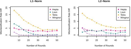
The results for both distance metrics can be seen in Figure 4. We see that while behavior varies slightly depending on the dataset, T = 40 iterations is a reasonable choice since the algorithms do not generally seem to converge further with more rounds. We will fix this parameter from here on, as it also exceeds the required amount of iterations for the exact version to converge.
10 20 30 40 50
0
5
10
15
20
L1−Norm
Number of Rounds
Misclassification Rate Diff
● ●
●
● ● ● ● ● ● ● ●
Hepta Lsun Tetra Wingnut
10 20 30 40 50
0
5
10
15
20
L2−Norm
Number of Rounds
Misclassification Rate Diff ● ● ●
● ● ● ●
● ● ● ●
Hepta Lsun Tetra Wingnut
Fig. 4.Average difference in misclassification rate between the stabilized and the exact algorithm (average % mislabeled stabilized) - (average % mislabeled exact).
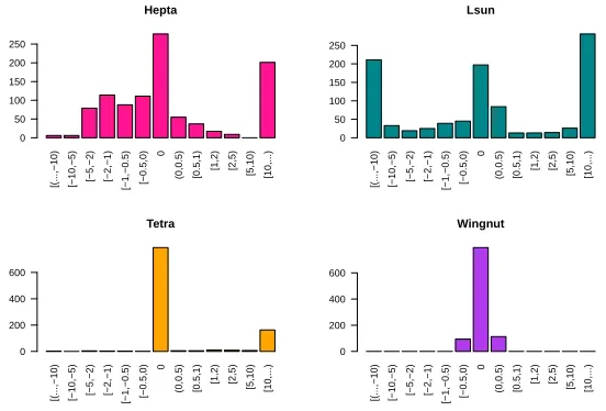
original algorithm, not with the intention of improving clustering accuracy, but rather to make it executable under an FHE scheme at all. This added function-ality naturally comes as a tradeoff, and we will now examine the magnitude of the loss in accuracy in Figure 5. The corresponding histogram for theL2-norm
can be found in Appendix B.1
[(...,−10) [−10,−5) [−5,−2) [−2,−1) [−1,−0.5) [−0.5,0)
0
(0,0.5) [0.5,1) [1,2) [2,5) [5,10) [10,...)
Hepta
0 50 100 150 200 250
[(...,−10) [−10,−5) [−5,−2) [−2,−1) [−1,−0.5) [−0.5,0)
0
(0,0.5) [0.5,1) [1,2) [2,5) [5,10) [10,...)
Lsun
0 100 200 300 400 500
[(...,−10) [−10,−5) [−5,−2) [−2,−1) [−1,−0.5) [−0.5,0)
0
(0,0.5) [0.5,1) [1,2) [2,5) [5,10) [10,...)
Tetra
0 200 400 600 800
[(...,−10) [−10,−5) [−5,−2) [−2,−1) [−1,−0.5) [−0.5,0)
0
(0,0.5) [0.5,1) [1,2) [2,5) [5,10) [10,...)
Wingnut
0 200 400 600 800
Fig. 5. Distribution of the difference in misclassification rate for stabilized vs. exact
K-Means-Algorithm (% mislabeled stabilized) - (% mislabeled exact)
,L1-norm.
stabilized version is actually slightly better than the original algorithm in about 30% of the cases. However, most of the time, we feel that there will be a slight performance decrease. The fact that there are some outliers where performance is drastically worse can easily be solved by running the algorithm several times in parallel, and only keeping the best run. This can be done under homomorphic encryption much like computing the minimum in Section 5.2, but will not be implemented in this paper.
Runtime While we will have a more detailed discussion of the runtime of all our algorithms in Section 7, we would like to already present the performance gain at this point: Recall that we estimated that running the exact algorithm from Section 4 would take almost 1.5 years. In contrast, our Stabilized Algorithm can be run in 25.93 days, or less than a month. This is less than 5% of the runtime of the exact version. Note that this is single-thread computation time on our computer, which could be greatly improved as detailed in Section 7 (though these improvements would apply to both algorithms, but we expect the ratio between the two algorithms to stay the same).
Conclusion In conclusion to this Section, we feel that by modifying the K -Means-Algorithm, we have traded a very small amount of accuracy for the ability to perform clustering on encrypted data in a more reasonable amount of time, which is a functionality that has not been achieved previously. The next section will deal with an idea to improve runtimes even more.
6
Approach 3: The Approximate Version
In this section, we present another modification which trades in a bit of accu-racy for slightly improved runtime: Since the Comparefunction is linear in the length of its inputs, speeding up this building block would make the entire com-putation more efficient. To do this, first recall that we encode our numbers in a bitwise fashion after having scaled them to integers. This means that we have access to the individual bits and can, for example, delete theS least significant bits, which corresponds to dividing the number by 2S and truncating. Let ˜X
denote this truncated version of a number X, and ˜Y that of a numberY. Then
Compare( ˜X,Y˜) =Compare(X, Y) if |X−Y| ≥2S, and may or may not return the correct result if |X −Y| < 2S. However, correspondingly, if the result is wrong, the centroid that is wrongly assigned to the data entry is no more than 2Sfurther from the data entry than the correct one. We propose to pick an initial
S and decrease it over the course of the algorithm, so that accuracy increases as we near the end. The exact workings of this approximate comparison, denoted
Algorithm 4:ApproxCompare(X, Y, S) Input:The two argumentsX, Y, encoded bitwise
Input:The accuracy factorS
// Corresponds to X˜=bX/2Sc
1 Remove lastSbits fromX, denote ˜X;
// Corresponds to Y˜ =bY /2Sc
2 Remove lastSbits fromY, denote ˜Y;
// Regular comparison function,C∈ {0,1}
3 C=Compare( ˜X,Y˜);
Output:C
6.1 Evaluation
In this section, we compare the performance of the stabilizedK-Means-Algorithm using this approximate comparison, denoted simply by “Approximate Version”, to the original and stabilizedK-Means-Algorithm on our data sets.
Accuracy Recall from Section 5.1 that we scaled the data with the factor 220
and truncated to obtain the input data. This means that for S = 5, a wrongly assigned centroid would be at most 25 further from the data entry than the
correct centroid on the scaled data - or no more than 2−15 on the original data
scale. We setS = min{7,(T /5)−1} where T is the number of iterations, and reduce S by one every 5 rounds. We again examine the average (over 1000 iterations) difference in the misclassification rate to both the exact algorithm and the stabilized algorithm.
10 20 30 40 50
0
5
10
15
20
L1−Norm
Number of Rounds
Misclassification Rate Diff
● ●
● ●
● ● ● ● ● ● ●
Hepta Lsun Tetra Wingnut
10 20 30 40 50
0
5
10
15
20
L2−Norm
Number of Rounds
Misclassification Rate Diff ● ● ●
● ●
● ● ● ● ● ●
Hepta Lsun Tetra Wingnut
Fig. 6.Average difference in misclassification rate between the approximate and the exact algorithm (average % mislabeled approximate) - (average % mislabeled exact)
The results for both distance metrics can be seen in Figures 6 and 7. We see that again, T = 40 iterations is a reasonable choice because the algorithms do not seem to converge further with more rounds.
10 20 30 40 50
0
1
2
3
4
5
6
L1−Norm
Number of Rounds
Misclassification Rate Diff
● ●
● ●
●
● ● ● ● ● ●
Hepta Lsun Tetra Wingnut
10 20 30 40 50
0
1
2
3
4
5
6
L2−Norm
Number of Rounds
Misclassification Rate Diff ● ●
● ● ● ● ● ●
● ● ●
Hepta Lsun Tetra Wingnut
Fig. 7. Average difference in misclassification rate for approximate vs. stabilized al-gorithm (average % mislabeled approximate) - (average % mislabeled stabilized).
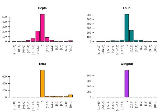
in Appendix B.1) and Figure 9 (for the approximate versus the stabilized K -Means-Algorithm, figures for theL2-norm in Appendix B.1).
[(...,−10) [−10,−5) [−5,−2) [−2,−1) [−1,−0.5) [−0.5,0)
0
(0,0.5) [0.5,1) [1,2) [2,5) [5,10) [10,...)
Hepta
0 50 100 150 200 250
[(...,−10) [−10,−5) [−5,−2) [−2,−1) [−1,−0.5) [−0.5,0)
0
(0,0.5) [0.5,1) [1,2) [2,5) [5,10) [10,...)
Lsun
0 50 100 150 200 250
[(...,−10) [−10,−5) [−5,−2) [−2,−1) [−1,−0.5) [−0.5,0)
0
(0,0.5) [0.5,1) [1,2) [2,5) [5,10) [10,...)
Tetra
0 200 400 600
[(...,−10) [−10,−5) [−5,−2) [−2,−1) [−1,−0.5) [−0.5,0)
0
(0,0.5) [0.5,1) [1,2) [2,5) [5,10) [10,...)
Wingnut
0 200 400 600
Fig. 8.Distribution of the difference in misclassification rate for approximate vs. exact
K-Means-Algorithm (% mislabeled approximate) - (% mislabeled exact)
,L1-norm.
We see that usually, the approximate version performs only slightly worse than the stabilized version. There is still the effect in the Lsun dataset that the approximate version outperforms the original K-Means-Algorithm in a signifi-cant amount of cases (though this effect mostly occurs for the L1-norm), but it
[(...,−10) [−10,−5) [−5,−2) [−2,−1) [−1,−0.5) [−0.5,0)
0
(0,0.5) [0.5,1) [1,2) [2,5) [5,10) [10,...)
Hepta
0 100 200 300 400 500
[(...,−10) [−10,−5) [−5,−2) [−2,−1) [−1,−0.5) [−0.5,0)
0
(0,0.5) [0.5,1) [1,2) [2,5) [5,10) [10,...)
Lsun
0 100 200 300 400 500 600
[(...,−10) [−10,−5) [−5,−2) [−2,−1) [−1,−0.5) [−0.5,0)
0
(0,0.5) [0.5,1) [1,2) [2,5) [5,10) [10,...)
Tetra
0 200 400 600
[(...,−10) [−10,−5) [−5,−2) [−2,−1) [−1,−0.5) [−0.5,0)
0
(0,0.5) [0.5,1) [1,2) [2,5) [5,10) [10,...)
Wingnut
0 200 400 600 800
Fig. 9.Distribution of the difference in misclassification rate for approximate vs. sta-bilizedK-Means-Algorithm (% mislabeled approx.) - (% mislabeled stab.)
,L1-norm.
Runtime We now examine how much gain in terms of runtime we have from this modification. Recall that it took about 1.5 years to run the exact algorithm, and 25.93 days to run the stabilized version. The approximate version runs in 25.79 days, which means a difference of about 210.7 minutes.
Obviously, the effect of the approximate comparison is not as big as an-ticipated. This is due to the bottleneck actually being the computation of the
L1-norm rather than theFindMin-procedure. Thus, for this specific application,
the approximate version may not be the best choice - however, for an algorithm that has a high number of comparisons relative to other operations, there can still be huge performance gains in terms of runtime. To see this, we ran just the comparison and approximate comparison functions with the same parameters as in our implementation of theK-Means-Algorithm (35 bits, 5 bits deleted for approximate comparison). The average (over 1000 runs each) runtime was 3.24 seconds for the regular comparison and 1.51 seconds for the approximate com-parison. We see that this does make a big difference, which is why we choose to present the modification even though the effect was outweighed by other bottle-necks in theK-Means-Algorithm computation.
7
Implementation Results
We now present the runtimes for the stabilized and approximate versions of the K-Means-Algorithm, along with the times for the exact version with the Fractional Encoding. Computations were done in a virtual machine with 20 GB of RAM and 4 virtual cores, running an Intel i7-3770 processor with 3.4 GHz. We used the TFHE library [38] without the SPQLIOS FMA-option, as our processor did not support this (runtimes might be faster when using this option).
The dataset we used was the Lsun dataset from [39], which consists of 400 rational data entries of 2 dimensions, andK= 3 clusters. We encoded the binary numbers with 35 bits and scaled to integers using 220(i.e., 20 bits were used for
the numbers after the decimal point). The timings we measured were for one round, and the approximate version used a deletion parameter ofS= 5. For the Fractional Encoding, the initial data was encoded with nominator in [211,212)
and denominator in roughly the same range, as the data is reasonable small. We also allotted 35 bits total for nominator and denominator each to allow a growth in required bitlength, and set the shortening parameter to 12, but shortened by 11 every once in a while (we derived this approach experimentally, see the discussion of the shortcoming of this approach in Section 4.4). The Fractional exact version was so slow that we ran it only on the first 10 data entries of the dataset - we will extrapolate the runtimes in Section 7.1.
7.1 Runtimes for the Entire Algorithm on a Single Core
In this subsection, we present the runtimes for the entireK-Means-Algorithm on encrypted data on our specific machine with single-thread computation. There is some extrapolation involved, as the measured runtimes were for one round (so we multiplied by the round number, which differs between the exact version and the other two, see Sections 5.3 and 6.1), and in the Fractional (exact) case, only for 10 data entries, so we multiplied that time by 40. Note that these times are with no parallelization, so there is much room for improvement as discussed in Section 7.2. The times can be found in Table 2.
Exact (Fractional) Stabilized Approximate
Runtime per Round 873.46 hours (36.39 days) 15.56 hours 15.47 hours
Rounds required 15 40 40
Total Runtime 545.91 days
≈17.95 months
25.93 days
≈0.85 months
25.79 days
≈0.85 months
Table 2.Single-thread runtimes (extrapolated) on our machine.
7.2 Further Speedup
At this point, we would like to address the subject of parallelism. At the moment (last accessed January 24th2018), the TFHE library only supplies single-thread computations - i.e., there is no parallelism. However, version 1.5 is expected soon, and this will allegedly support multithreading. We first explain why this would make an enormous difference for the runtime, and then quantify the involved timings.
Parallelism Looking at all our versions of the K-Means-Algorithm, it is easy to see that they are highly parallelizable: The Cluster Assignment step triv-ially so over the data entries (without any time needed for recombination of the individual results), and theMove Centroidssimilarly over the cluster centroids (the latter could also be parallelized over the data entries with a little recom-bination effort, which should still be negligible compared to the total running time). Since both steps are linear in the number K of centroids, the number
m of data entries, and the number T of round iterations, we thus present our runtimes in this subsection asper centroid, per data entry, per round, per core. This allows a more flexible estimate for when multithreading is supported, as the ability to actually use our 4 allotted cores would lead to only about 1/4 of the total runtimes presented in Section 7.1.
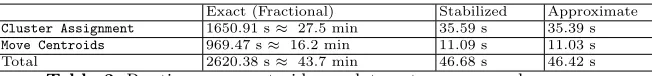
Round Runtimes We now present the runtime results for each of the three variants on encrypted data per centroid, per data entry, per round, per core in Table 3. We do not include runtimes for encoding/encryption and decryp-tion/decoding, as these would be performed on the user side, whereas the com-putation would be outsourced (encoding/encryption is ca. 1.5 seconds, and de-coding/decryption is around 5 ms). We see that the Fractional Encoding is ex-tremely slow, which motivated the Stabilized Algorithm in the first place.
Exact (Fractional) Stabilized Approximate
Cluster Assignment 1650.91 s≈ 27.5 min 35.59 s 35.39 s
Move Centroids 969.47 s≈ 16.2 min 11.09 s 11.03 s
Total 2620.38 s≈ 43.7 min 46.68 s 46.42 s
Table 3.Runtimes per centroid, per data entry, per round, per core.
References
1. Aggarwal, C.C., Hinneburg, A., Keim, D.A.: On the surprising behavior of distance metrics in high dimensional spaces. In: ICDT (2001)
3. Armknecht, F., Katzenbeisser, S., Peter, A.: Group homomorphic encryption: char-acterizations, impossibility results, and applications. DCC (2013)
4. Barnett, A., Santokhi, J., Simpson, M., Smart, N.P., Stainton-Bygrave, C., Vivek, S., Waller, A.: Image classification using non-linear support vector machines on encrypted data. IACR Cryptology ePrint Archive (2017/857)
5. Bonte, C., Vercauteren, F.: Privacy-preserving logistic regression training. IACR Cryptology ePrint Archive 233 (2018)
6. Bos, J.W., Lauter, K.E., Naehrig, M.: Private predictive analysis on encrypted medical data. Journal of Biomedical Informatics 50 (2014)
7. Bost, R., Popa, R.A., Tu, S., Goldwasser, S.: Machine learning classification over encrypted data. In: NDSS (2015)
8. Brakerski, Z., Gentry, C., Vaikuntanathan, V.: Fully homomorphic encryption without bootstrapping. ECCC 18 (2011)
9. Bunn, P., Ostrovsky, R.: Secure two-party k-means clustering. In: CCS (2007) 10. Chabanne, H., de Wargny, A., Milgram, J., Morel, C., Prouff, E.:
Privacy-preserving classification on deep neural network. IACR Cryptology ePrint Archive (2017/035)
11. Chen, H., Laine, K., Player, R.: Simple encrypted arithmetic library - SEAL v2.1. IACR Cryptology ePrint Archive 2017, 224 (2017)
12. Chillotti, I., Gama, N., Georgieva, M., Izabach`ene, M.: Faster fully homomorphic encryption: Bootstrapping in less than 0.1 seconds. In: ASIACRYPT (2016) 13. Coron, J., Lepoint, T., Tibouchi, M.: Scale-invariant fully homomorphic encryption
over the integers. In: PKC (2014)
14. Coron, J., Naccache, D., Tibouchi, M.: Public key compression and modulus switch-ing for fully homomorphic encryption over the integers. In: EUROCRYPT (2012) 15. van Dijk, M., Gentry, C., Halevi, S., Vaikuntanathan, V.: Fully homomorphic
en-cryption over the integers. In: EUROCRYPT (2010)
16. Ducas, L., Micciancio, D.: FHEW: bootstrapping homomorphic encryption in less than a second. In: EUROCRYPT (2015)
17. Esperan¸ca, P.M., Aslett, L.J.M., Holmes, C.C.: Encrypted accelerated least squares regression. In: Singh, A., Zhu, X.J. (eds.) AISTATS (2017)
18. Fan, J., Vercauteren, F.: Somewhat practical fully homomorphic encryption. IACR Cryptology ePrint Archive (2012/144)
19. Gentry, C.: A fully homomorphic encryption scheme. Ph.D. thesis, Stanford Uni-versity (2009)
20. Gentry, C., Sahai, A., Waters, B.: Homomorphic encryption from learning with errors: Conceptually-simpler, asymptotically-faster, attribute-based. In: CRYPTO (2013)
21. Gilad-Bachrach, R., Dowlin, N., Laine, K., Lauter, K.E., Naehrig, M., Wernsing, J.: Cryptonets: Applying neural networks to encrypted data with high throughput and accuracy. In: ICML (2016)
22. Graepel, T., Lauter, K.E., Naehrig, M.: ML confidential: Machine learning on en-crypted data. In: ICISC (2012)
23. Halevi, S., Shoup, V.: Algorithms in helib. In: CRYPTO (2014)
24. Jagannathan, G., Pillaipakkamnatt, K., Wright, R.N., Umano, D.: Communication-efficient privacy-preserving clustering. Trans. Data Privacy (2010)
25. Jagannathan, G., Wright, R.N.: Privacy-preserving distributed k-means clustering over arbitrarily partitioned data. In: SIGKDD (2005)
27. J¨aschke, A., Armknecht, F.: (finite) field work: Choosing the best encoding of numbers for fhe computation. In: CANS (2017)
28. Jha, S., Kruger, L., McDaniel, P.D.: Privacy preserving clustering. In: ESORICS (2005)
29. Kim, A., Song, Y., Kim, M., Lee, K., Cheon, J.H.: Logistic regression model train-ing based on the approximate homomorphic encryption. IACR Cryptology ePrint Archive (254) (2018)
30. Kim, M., Song, Y., Wang, S., Xia, Y., Jiang, X.: Secure logistic regression based on homomorphic encryption. IACR Cryptology ePrint Archive (074) (2018) 31. Liu, X., Jiang, Z.L., Yiu, S., Wang, X., Tan, C., Li, Y., Liu, Z., Jin, Y., Fang, J.:
Outsourcing two-party privacy preserving k-means clustering protocol in wireless sensor networks. In: MSN (2015)
32. Lu, W., Kawasaki, S., Sakuma, J.: Using fully homomorphic encryption for statis-tical analysis of categorical, ordinal and numerical data. IACR Cryptology ePrint Archive (2016/1163)
33. MacQueen, J., et al.: Some methods for classification and analysis of multivariate observations. In: Proceedings of the fifth Berkeley symposium on mathematical statistics and probability (1967)
34. Meskine, F., Bahloul, S.N.: Privacy preserving k-means clustering: a survey re-search. Int. Arab J. Inf. Technol. (2012)
35. Naehrig, M., Lauter, K.E., Vaikuntanathan, V.: Can homomorphic encryption be practical? In: CCSW (2011)
36. Phong, L.T., Aono, Y., Hayashi, T., Wang, L., Moriai, S.: Privacy-preserving deep learning via additively homomorphic encryption. IACR Cryptology ePrint Archive (2017/715)
37. Smart, N.P., Vercauteren, F.: Fully homomorphic encryption with relatively small key and ciphertext sizes. In: PKC (2010)
38. TFHE Library: https://tfhe.github.io/tfhe
39. Ultsch, A.: Clustering with som: U*c. In: Proc. Workshop on Self-Organizing Maps (2005)
40. Vaidya, J., Clifton, C.: Privacy-preservingk-means clustering over vertically par-titioned data. In: SIGKDD (2003)
41. Wu, D.J., Feng, T., Naehrig, M., Lauter, K.E.: Privately evaluating decision trees and random forests. PoPETs (4) (2016)
42. Xing, K., Hu, C., Yu, J., Cheng, X., Zhang, F.: Mutual privacy preserving $k$ -means clustering in social participatory sensing. IEEE Trans. Industrial Informatics (2017)
A
Function Building Blocks
In this section, we present some building blocks used in our algorithms.
A.1 Taking the Absolute Value
Algorithm 5:Absolute Value
Input:Valuea=an. . . a1a0in binary encoding // Set the conditional variable as the MSB 1 C=M SB(a) =an;
// Apply the MUX gate 2 d=M U X(C,−a, a);
// IfC= 1, i.e., a is negative, d=−a. If C= 0, i.e., a is positive, d=a. So
d=|a|.
Output:d
A.2 Comparison
While comparison is not natively supported by FHE schemes, it can be built from additions and multiplications. We will detail how to do this for Two’s Complement Encoding. We first show how to compare two natural numbers in Algorithm 6, and then use that as a building block to compare signed numbers.
Algorithm 6:NatComp(a, b) Input:Natural numbera=an. . . a1a0
Input:Natural numberb=bn. . . b1b0
// Set result to0
1 res= 0; 2 fori= 0tondo
// Set temp to0if ai6=bi and to 1if ai=bi
3 temp=XN OR(ai, bi);
// Iftemp= 1(inputs are equal), don’t change res. If temp= 0(inputs are
unequal), set res=bi
4 res=M U X(temp, res, bi);
5 end
//res= 1⇔a < b Output:res
The idea4 is that the variable res is set to 0 and then in each iteration of
the for-loop it denotes the result of the comparison on the previous bits. Thus, if the two bits at positioniare equal (ai=bi), the resultresof the comparison does not change. If they are unequal, the lower bits do not matter anymore and the result is set to res=bi. This works because ifbi = 1, that means ai = 0, so the numberai. . . a1a0is smaller thanbi. . . b1b0. Thus the outcome should be
1 =bi. If, on the other hand,bi = 0, then ai=1 and the numberai. . . a1a0 is
larger thanbi. . . b1b0, so the outcome is 0 =bi.
We now use this comparison of natural numbers as a building block when comparing signed numbers (concretely, in Two’s Complement encoding), as can be seen in Algorithm 7.
As can easily be verified, the formula in Line 2 evaluates tocifan =bn, i.e., the signs are equal – in this case, the result ofNatComp(a, b) is correct. Ifan = 0 andbn= 1, i.e.,bis negative andais positive, the formula evaluates to 0, which
4
Algorithm 7:Compare(a, b) Input:Signed numbera=an. . . a1a0
Input:Signed numberb=bn. . . b1b0
// Compare as if natural numbers, result is correct if signs are equal
1 c=NatComp(a, b);
// The sign bits arean andbn
2 res=an·(bn+ 1) + (an+bn+ 1)·c;
Output:res
is correct because b < a. Lastly, if an= 1 andbn = 0, i.e.,bis positive andais negative, the formula evaluates to 1, which is also correct becausea < b.
B
Supplemental Figures
This section presents some supplemental Figures.
B.1 Histograms for L2-Norm
We now present the counterparts of the performance histograms for theL2-norm.
Stabilized versus Exact Here, we present Figure 10, which compares the per-formance of the stabilized to the original algorithm, for theL2 distance metric.
The original figure for theL1-norm is Figure 5 on page 18.
[(...,−10) [−10,−5) [−5,−2) [−2,−1) [−1,−0.5) [−0.5,0)
0
(0,0.5) [0.5,1) [1,2) [2,5) [5,10) [10,...)
Hepta
0 50 100 150 200 250 300
[(...,−10) [−10,−5) [−5,−2) [−2,−1) [−1,−0.5) [−0.5,0)
0
(0,0.5) [0.5,1) [1,2) [2,5) [5,10) [10,...)
Lsun
0 50 100 150 200 250 300 350
[(...,−10) [−10,−5) [−5,−2) [−2,−1) [−1,−0.5) [−0.5,0)
0
(0,0.5) [0.5,1) [1,2) [2,5) [5,10) [10,...)
Tetra
0 200 400 600 800
[(...,−10) [−10,−5) [−5,−2) [−2,−1) [−1,−0.5) [−0.5,0)
0
(0,0.5) [0.5,1) [1,2) [2,5) [5,10) [10,...)
Wingnut
0 200 400 600
Fig. 10.Distribution of the difference in misclassification rate for stabilized vs. exact
K-Means-Algorithm (% mislabeled stabilized) - (% mislabeled exact)
Approximate versus Exact We now do the same thing for Figure 8, which compares the approximate to the exact version.
[(...,−10) [−10,−5) [−5,−2) [−2,−1) [−1,−0.5) [−0.5,0)
0
(0,0.5) [0.5,1) [1,2) [2,5) [5,10) [10,...)
Hepta
0 50 100 150 200 250
[(...,−10) [−10,−5) [−5,−2) [−2,−1) [−1,−0.5) [−0.5,0)
0
(0,0.5) [0.5,1) [1,2) [2,5) [5,10) [10,...)
Lsun
0 50 100 150 200 250
[(...,−10) [−10,−5) [−5,−2) [−2,−1) [−1,−0.5) [−0.5,0)
0
(0,0.5) [0.5,1) [1,2) [2,5) [5,10) [10,...)
Tetra
0 200 400 600
[(...,−10) [−10,−5) [−5,−2) [−2,−1) [−1,−0.5) [−0.5,0)
0
(0,0.5) [0.5,1) [1,2) [2,5) [5,10) [10,...)
Wingnut
0 200 400 600
Fig. 11.Distribution of the difference in misclassification rate for approximate vs. exact
K-Means-Algorithm (% mislabeled approximate) - (% mislabeled exact)
Approximate versus Stabilized Lastly, we also present the counterpart of Figure 9, comparing the approximate to the stabilized version, for theL2-norm
in Figure 12.
[(...,−10) [−10,−5) [−5,−2) [−2,−1) [−1,−0.5) [−0.5,0)
0
(0,0.5) [0.5,1) [1,2) [2,5) [5,10) [10,...)
Hepta
0 100 200 300 400 500 600
[(...,−10) [−10,−5) [−5,−2) [−2,−1) [−1,−0.5) [−0.5,0)
0
(0,0.5) [0.5,1) [1,2) [2,5) [5,10) [10,...)
Lsun
0 50 100 150 200 250 300
[(...,−10) [−10,−5) [−5,−2) [−2,−1) [−1,−0.5) [−0.5,0)
0
(0,0.5) [0.5,1) [1,2) [2,5) [5,10) [10,...)
Tetra
0 200 400 600
[(...,−10) [−10,−5) [−5,−2) [−2,−1) [−1,−0.5) [−0.5,0)
0
(0,0.5) [0.5,1) [1,2) [2,5) [5,10) [10,...)
Wingnut
0 200 400 600 800
Fig. 12. Distribution of the difference in misclassification rate for approximate vs. stabilized K-Means-Algorithm (% mislabeled approx.) - (% mislabeled stab.), L2