Computing supersingular isogenies on Kummer surfaces
Craig Costello
Microsoft Research, USA [email protected]
Abstract. We apply Scholten’s construction to give explicit isogenies between the Weil restriction of supersingular Montgomery curves with full rational 2-torsion over Fp2 and
corresponding abelian surfaces overFp. Subsequently, we show that isogeny-based public key cryptography can exploit the fast Kummer surface arithmetic that arises from the theory of theta functions. In particular, we show that chains of 2-isogenies between elliptic curves can instead be computed as chains of Richelot (2,2)-isogenies between Kummer surfaces. This gives rise to new possibilities for efficient supersingular isogeny-based cryptography.
Keywords: Supersingular isogenies, SIDH, Kummer surface, Richelot isogeny, Scholten’s construction.
1
Introduction
Public key cryptography based on supersingular isogenies is gaining increased popularity due to its conjectured quantum-resistance. In November 2017, an actively secure key encapsulation mechanism called SIKE [22], which is based on Jao and De Feo’s supersingular isogeny Diffie-Hellman (SIDH) protocol [23,16], was submitted to NIST in response to their call for quantum-resistant public key solutions [34]. When compared to other proposals of quantum-quantum-resistant key encapsulation mechanisms, SIKE currently offers an interesting bandwidth versus performance trade-off; its keys are appreciably smaller than its code- and lattice-based counterparts, but the times required for encapsulation and decapsulation are significantly higher. This performance drawback of supersingular isogeny-based cryptography is the main practical motivation for this paper.
This work. 15 years ago, Scholten [31] showed that if E is an elliptic curve defined over a quadratic extension field Lof a non-binary fieldK, and if its entire 2-torsion is L-rational, then a genus-2 curveC can be constructed overK such that its Jacobian JC is isogenous to the Weil
restriction ResLK(E). Fortuitously, supersingular isogeny-based cryptography currently uses ellip-tic curves that precisely meet these requirements. In parellip-ticular, state-of-the-art implementations (e.g., [14,15]) of SIDH fix a large prime field K = Fp with p = 2i3j−1 for i > j >100,
con-struct L = Fp2, and work in the supersingular isogeny class of elliptic curves over Fp2 whose
group structures are all isomorphic toZp+1×Zp+1. This necessarily means that all curves in the
supersingular isogeny class have full rational 2-torsion, can be written in Montgomery form, and that for any such curveE/Fp2, Scholten’s construction can be used to write down the curveC/Fp
whose JacobianJC is isogenous to the Weil restriction ofE with respect toFp2/Fp.
Fp2. In particular, rather than using V´elu’s formulas [35] to compute secret 2e-isogenies as chains
of 2- and/or 4-isogenies on elliptic curves overFp2 [16], we show that the same secret isogenies can
instead be computed as a chain of (2,2)-isogenies on Jacobian varieties overFp. While computing
isogenies on higher genus abelian varieties is, in general, much more complicated than V´elu’s formulas for elliptic curve isogenies, the special case of (2,2)-isogenies between genus-2 Jacobians dates back to the works of Richelot [29,30] from almost two centuries ago. Subsequently, the computation of Richelot isogenies is already well-documented in the literature (cf. [10,33]), and this allows us to tailor the explicit formulas to our scenario of computing chains of (2,2)-isogenies on supersingular Jacobians.
Crucial to the efficacy of this work is that we are able to compute (2,2)-isogenies on the Kum-mer surfaces associated to supersingular Jacobians, rather than in the full Jacobian groups. This allows us to leverage the fast Kummer surface arithmetic arising from the classical theory of theta functions, which was first proposed for computational purposes by the Chudnovsky brothers [12], and which was brought to life in cryptography by Gaudry [19]. In his article [19, Remark 3.5], Gaudry points out that the fast (pseudo-)doublings on Kummer surfaces are the result of pushing points back and forth through a (2,2)-isogenous variety, i.e., that the corresponding (2,2)-isogenies split the multiplication-by-2 map on the associated Kummer surface. This observation plays a key role in deriving efficient isogenies on fast Kummer surfaces.
Related work. This paper relies on the results of several
authors:-– The construction in Scholten’s unpublished manuscript [31] is at the heart of this work. It gives rise to Proposition 1 which paves the way for the rest of the paper.
– In 2014, Bernstein and Lange [6] revived Scholten’s work when they proposed using his con-struction in the context of (hyper)elliptic curve cryptography (H)ECC to convert keys back and forth between elliptic and hyperelliptic curves, in such a way so as to exploit advantageous properties of both settings. They were also the first to explicitly derive instances of the isoge-nies alluded to by Scholten, and to show that they can be efficient enough to be used in online cryptographic computations. The setting considered in [6] has the advantage of having a single elliptic-and-hyperelliptic curve pair that is fixed once-and-for-all (meaning the back-and-forth maps also remain fixed), while in our scenario we will need general-purpose maps that can handle any supersingular Montgomery curves efficiently at runtime. However, in the super-singular setting, we have the advantage that our Jacobians have a fixed embedding degree of k= 2, and we can therefore exploit the existence of an efficiently computabletrace map; this allows us to derive much simpler back-and-forth isogenies than those presented in [6].
– Renes and Smith [28] recently introduced qDSA: the quotient digital signature algorithm. In order to instantiate their scheme on fast Kummer surfaces, they deconstructed the pseudo-doubling map into the explicit (2,2)-isogenies alluded to by Gaudry [19, Remark 3.5]; this deconstruction (depicted in [28, Figure 1]) plays a key role in this paper. Indeed, it was their explicit treatment of the dual Kummer surface and subsequent illustration of simple (2, 2)-isogenies between fast Kummer surfaces that, in part, inspired the present work.
means that when we move to genus 2, we are able to work in the pre-existing SIDH infrastruc-ture and replace abelian surfaces with Kummer surfaces and points on abelian surfaces with points on these Kummer surfaces.
– One significant hurdle to overcome in order to exploit fast isogenies on our Kummer surfaces it that the (2,2)-isogeny that splits pseudo-doublings1 corresponds to a special kernel, and in SIDH computations we need isogenies that work identically for general kernel elements, or at least identically for all of the kernel elements that can arise in a large-degree supersingular isogeny routine. This was achieved in the elliptic curve case by De Feo, Jao and Plˆut [16], who use an isomorphism to move thegeneral Montgomery 2-torsion point (α,0) withα6= 0 to the special 2-torsion point (0,0). However, in our case, the kernels of Richelot isogenies are non-cyclic, and finding the isomorphism to move general kernels to special kernels is less obvious. Our overcoming this hurdle on Jacobians (see Section 4) is aided by the use of quadratic splittings introduced by Smith in his treatment of Richelot kernels [33, Chapter 8], and our overcoming this hurdle on fast Kummer surfaces (see Section 5) employs the technique of [16,
§4.3.2], which uses higher order torsion points (lying above the kernel) to avoid square root computations.
Roadmap. Section 2 provides background and sets notation. Section 3 defines the abelian surfaces corresponding to supersingular Montgomery curves (by way of Proposition 1), and gives the back-and-forth maps between these two objects. Section 4 then studies (2,2)-isogenies on supersingular abelian surfaces and, in particular, it shows how to replace even-power elliptic curve isogenies defined over Fp2 with chains of (2,2)-isogenies inside full Jacobians defined over Fp. This lays
the foundations to move to Kummer surfaces in Section 5, where the (2,2)-isogenies simplify and become much faster. Implications for isogeny-based cryptography are discussed in Section 6.
There are many constants, variables and formulas in this work, so the risk of typographical error is high. Thus, for readers wanting to verify or replicate this work, illustrative Magma source files can be found at
https://www.microsoft.com/en-us/download/details.aspx?id=57309.
Before going any further, we stress that this paper in no way changes the security picture of isogeny-based cryptography, and that using Kummer surfaces overFp instead of elliptic curves over Fp2
can be viewed as a mere implementation choice. The efficient back-and-forth maps in Section 3 show that any conceivable hard problem that can be posed in one setting can be efficiently ported over to the other setting.
Acknowledgements. Big thanks to Joost Renes for his help in ironing out some kinks on the Kummer surfaces, to Michael Naehrig for several helpful discussions during the preparation of this work, and to the anonymous reviewers for their useful comments.
2
Preliminaries
This section gives the necessary background for the remainder of the paper. We start with a brief summary of some jargon for non-experts. An abelian variety is a general term for a projective algebraic variety that possesses an algebraic group law. When we quotient an abelian variety by the map that takes elements to their inverses, we get the associated Kummer variety. There are two examples that are relevant in this paper. Anelliptic curve is an abelian variety of dimension 1, and its quotient by {±1} gives the associated Kummer line; if E is a short Weierstrass or Montgomery curve, then a geometric point P ∈ E can be parameterised on the Kummer line
1
E/{±1} by its x-coordinate, x(P), which is why it is often called thex-line. An abelian surface
is an abelian variety of dimension 2, and all such instances in this work occur as Jacobian groups of genus-2 hyperelliptic curves; if C is a genus-2 curve andJC is its Jacobian, then the quotient
JC/{±1} is called aKummer surface.
Supersingular Montgomery curves. State-of-the-art SIDH implementations (cf. [14,15]) cur-rently employ large prime fields of the form p = 2i3j−1 with i > j >100, so that, over Fp2,
the supersingular isogeny class consists entirely of curves whose abelian group structure is isomor-phic to Zp+1×Zp+1. This necessarily means that all of the curves in the isogeny class have full
Fp2-rational 2-torsion, and moreover, that they can be written in Montgomery form over Fp2 as
By2 =x3+Ax2+x. Rather than parameterising Montgomery curves in this way, we will make an arbitrary choice of one of the two rational 2-torsion points (α,0) withα /∈ {−1,0,1}(the other is (1/α,0)), and from hereon will useEαto denote the curve
Eα/K:y2=x(x−α)(x−1/α), (1)
thej-invariant of which is
j(Eα) = 256
(α4−α2+ 1)3 α4(α2−1)2 .
Note that thej-invariant is the same for Eα as it is for the curveδy2 =x(x−α)(x−1/α); this
is becauseδonly helps fix the quadratic twist, i.e., only fixes the curve up to ¯K-isomorphism. As mentioned in Section 1, point and isogeny arithmetic is independent ofδ, so our curves need only be defined up to twist.
Throughout the paper we will often be making implicit use of the following result, which is essentially due to Auer and Top [1].
Lemma 1. If Eα/Fp2: y2=x(x−α)(x−1/α) is supersingular, thenα∈(F×p2)
2, and α2−1 ∈
(F×p2)8.
Proof. The group structure ofEαimplies that at least one of the three 2-torsion points (0,0), (α,0)
and (1/α,0) must be in [2]E(Fp2), soα∈(F×p2)2by [1, Lemma 2.1]. Thus, there exists∈Fp2 such
that2=−α3, and it follows thatEis isomorphic over
Fp2to the curve ˜E:y2=x(x−1)(x+α2−1)
via (x, y)7→(−αx+ 1, y). Applying [1, Proposition 3.1] yields thatα2−1∈(
F×p2)8. ut
Abelian surfaces. Over a field K of characteristic not 2, every genus-2 curve is birationally equivalent to a curve of the form C: y2 = f(x), where f(x) ∈ K[x] is of degree 6 and has no repeated factors. In this work we will only encounter such curves wheref(x) splits completely in K[x], so we will often be writing them in the form
C/K:y2= (x−z1)(x−z2)(x−z3)(x−z4)(x−z5)(x−z6), (2)
where zi ∈K fori∈ {1, . . . ,6}, and where we writey2 instead ofδy2 for the same reason as for
the elliptic curve case above.
Denote the differencezi−zj by (ij). Following Igusa [21, p. 620], define the quantities
I2:=
X
(12)2(34)2(56)2,
I4:=
X
(12)2(23)2(31)2(45)2(56)2(64)2,
I6:=
X
(12)2(23)2(31)2(45)2(56)2(64)2(14)2(25)2(36)2,
I10:=
Y
(12)2, (3)
and they play an analogous role to thej-invariant of an elliptic curve: two curvesC andC0, with
respective Igusa-Clebsch invariants (I2, I4, I6, I10) and (I20, I40, I60, I100 ), are isomorphic over ¯Kif and only if
(I2:I4:I6:I10) = (I20:I
0
4:I
0
6:I
0
10)∈P(2,4,6,10)( ¯K),
i.e., if and only if there exists a λ ∈ K¯× such that (I20, I40, I60, I100 ) = (λ2I
2, λ4I4, λ6I6, λ10I10). Observe that, as in the elliptic curve case, the invariants here are independent of δ, i.e., are twist-independent. Fora, b, c, d∈K withad6=bcande∈K×, the map
κ(a,b,c,d): C→C0, (x, y)7→
ax+b
cx+d, ey (cx+d)3
(4)
is a K-rational isomorphism to the curve C0. Up to isomorphism and quadratic twist, and by abuse of notation, we can writeC0 asC0:y2=Q6
i=1(x−zi0), where z0i= (azi+b)/(czi+d). Let {`0, `1, `∞, `λ, `µ, `ν}={z1, . . . , z6}be some relabeling of the roots of the sextic in (2). Setting
a=`1−`∞, b=`0(`∞−`1), c=`1−`0, and d=`∞(`0−`1)
in (4) yields a mapκ(a,b,c,d): C→Cλ,µ,ν, where
Cλ,µ,ν:y2=x(x−1)(x−λ)(x−µ)(x−ν)
is the so-calledRosenhain formofC. Underκ(a,b,c,d), the points (`λ,0), (`µ,0) and (`ν,0) onCare
respectively sent to (λ,0), (µ,0) and (ν,0) onCλ,µ,ν, while the points (`0,0), (`1,0) and (`∞,0) are
respectively sent to (0,0), (1,0), andthe point at infinity onCλ,µ,ν. There are 6! = 720 possible
relabelings of the sixzi, and as such there are 720 possible (ordered) triples (λ, µ, ν) ofRosenhain
invariants. In this work we can and will identify the Jacobian variety, JC, of the curveC/Kwith
the degree zero divisor class group ofC, i.e., with Pic0K(C) = Div0K(C)/PrinK(C) (cf. [18, §7.8]).
In this way a point in the affine part of JC (see [18, p. 204]) is represented using the Mumford
representation of the corresponding divisorD∈Pic0K(C); ifD is reduced and non-zero, then the effective component of the support ofD either contains 1 or 2 (not necessarily unique) ¯K-rational points on C. In the first (so-called degenerate) case, if (x1, y1) is the only such point (and its multiplicity is 1) in the support of D, then (x1, y1)∈ C(K), and its Mumford representation is (x−x1, y1)∈ K[x]×K[x]. In the general case, when (x1, y1) and (x2, y2) with x1 6=x2 are the two ¯K-rational points onC in supp(D), then the corresponding Mumford representation is
(x2+u1x+u0, v1x+v0)∈K[x]×K[x],
where
u1=−x1−x2, u0=x1x2, v1=
y2−y1 x2−x1
, and v0=
y1x2−x1y2 x2−x1
. (5)
Note that, in general, the Mumford representation of a point inJC(K) can always be written in
K[x]×K[x], but this does not imply that the underlying points onC( ¯K) areK-rational. If (x2+u
1x+u0, v1x+v0) is a generic point inJC, then the map κ(a,b,c,d): C →C0 in (4) induces a map between their Jacobians, where, for elements with `1 = c2u0−cdu1 +d2 and `2 =ad−bcsuch that`1`2= 0, we have (6 x2+u1x+u0, v1x+v0)7→(x2+u01x+u00, v01x+v00), with
u01=`−11((ad+bc)u1−2acu0−2bd), u00=`
−1 1 a
2u
0−abu1+b2
,
v00=−e(`21`2)−1 ac2(u0u1v1−u21v0+u0v0)−c(2ad+bc)(u0v1−u1v0)−d(ad+ 2bc)v0+bd2v1
,
Weil restriction of scalars. The Weil restriction of scalars is the process of re-writing a system of equations over a finite extensionL/K as a system of equations in more variables overK – we refer to [18, §5.7] for a more general discussion. In this work it can be considered as merely a formality to increase dimension so that speaking of isogenies makes sense. The Weil restriction of our one-dimensional varieties Eα/Fp2 (with respect to the extension Fp2 =Fp(i) withi2+ 1) is
the two-dimensional variety
Wα:= Res
Fp2
Fp (Eα) =V
W0(x0, x1, y0, y1), W1(x0, x1, y0, y1)
,
where
W0= (α20+α21) α0(x02−x21)−2α1x0x1+δ0(y02−y21)−2y0y1δ1−x0(x20−3x21+ 1)
+α0(x20−x12) + 2α1x0x1 and
W1= (α20+α 2 1) α1(x
2 0−x
2
1) + 2α0x0x1+δ1(y02−y 2
1) + 2y0y1δ0−x1(3x20−x 2 1+ 1)
+α1(x21−x 2
0) + 2α0x0x1
are obtained by puttingx=x0+x1·i,y=y0+y1·ias well asα=α0+α1·iandδ=δ0+δ1·i (withx0, x1, y0, y1, α0, α1, δ0, δ1∈Fp) into (1). In terms of dimension, it now makes sense to speak
of isogenies betweenWα and the two-dimensional abelian surfaces described in the next section.
We make the disclaimer that oftentimes we will speak loosely and refer to isogenies and maps between Eα, intermediate curves, and abelian surfaces, but that from hereon it should be clear
that, technically speaking, these maps are only well-defined when speaking of the corresponding Weil restrictions of these elliptic curves with respect toFp2/Fp.
Power-of-2 elliptic curve isogenies in SIDH. Understanding how 2e-isogenies are computed in SIDH is key in understanding the directions we take in Section 4 and Section 5. Recall the three 2-torsion points onEαas (0,0), (α,0) and (1/α,0); in general, each of these corresponds to
a different 2-isogeny emanating fromEα. Following [16,§4.3.2] and [27,§4.2], when the kernel is
generated by the special point (0,0), applying V´elu’s formulas [35] to write down the isogeny allows us to (re)write the image curve in Montgomery form2. However, when the kernel is generated by one of the other two points, direct application of V´elu’s formulas makes writing the image curve in Montgomery form much less obvious. This was achieved in [16,27] by using an isomorphism to move these two kernel points to (0,0) on an isomorphic curve (which differs depending whether the kernel ish(α,0)iorh(1/α,0)i), prior to invoking V´elu.
In our case we follow an analogous path. From the work in [28], we have a very simple Kummer surface isogeny that corresponds to a special kernelO, and we use an isomorphism to move our two more general kernels, Υ and ˜Υ, prior to applying the isogeny (see sections 4 and 5 for the definitions ofO,Υ and ˜Υ).
We point out that this analogue is not a coincidence, and is made concrete in Lemma 2. Moreover, just like in the elliptic curve case where (0,0) cannot arise as the kernel of a repeated isogeny in SIDH (because it gives rise to the dual isogeny – see [16]), in our case it is O that corresponds to the dual so our kernel will, with the possible exception of the very first (2, 2)-isogeny, only ever correspond toΥ and ˜Υ.
3
Abelian surfaces isogenous to supersingular Montgomery curves
This section links supersingular Montgomery curves defined overFp2 with abelian surfaces defined
over Fp. We start with Proposition 1, which writes down the genus-2 curveCα/Fp arising from
Scholten’s construction; its proof is postponed until after we have derived the back-and-forth (2, 2)-isogenies between the given Weil restriction and abelian surface. We point out that the exposition
below is simplified by assuming3 p≡3 mod 4 so that
Fp2 =Fp(i) withi2+ 1 = 0, but treating
the complimentary or general case is analogous. The only impactful restriction made in addition to Scholten’s requirements is that of supersingularity. As mentioned in Section 1, this gives rise to simpler maps than those in [6] by way of the trace map, but several of our intermediate steps may still be useful beyond the supersingular scenario.
Proposition 1. Let p≡3 mod 4, letFp2 =Fp(i)withi2+ 1 = 0, and let
Eα/Fp2:y2=x(x−α)(x−1/α)
be supersingular with α 6∈ Fp. Write α= α0+α1·i with α0, α1 ∈ Fp. The Weil restriction of
scalars of Eα(Fp2)with respect toFp2/Fp is(2,2)-isogenous to the Jacobian, JCα, of
Cα/Fp:y2=f1(x)f2(x)f3(x), (7)
where
f1(x) =x2+2α0 α1
·x−1,
f2(x) =x2−2α0
α1
·x−1, and
f3(x) =x2−2α0(α
2
0+α21−1) α1(α2
0+α21+ 1)
·x−1.
Remark 1 (Singular quadratic splittings and split Jacobians).We immediately point out that the fi(x) in Proposition 1 are linearly dependent; namely,f3(x) = 1/(N+ 1)·f1(x) +N/(N+ 1)·f2(x),
whereN =NF
p2/Fp(α) =α 2 0+α
2
1. Oftentimes in the literature, this is referred to as the singular scenario, where the Jacobian of Cα is reducible, or split (e.g., [10, Theorem 14.1.1(ii)] and [33,
Proposition 8.3.1]). However, we stress that those results do not necessarily imply that this splitting occurs overFp; Cassels and Flynn assume that they are working in the algebraic closure [10, p. 154]
and Smith’s construction of the linear polynomials on [33, p. 119] also requires a field extension in the general case. Indeed, if all of the elliptic curves in our isogeny graph were (2,2)-isogenous to a Jacobian that is split overFp, this would have serious implications on the quantum security of
SIDH (see [11]). We conjecture that the Jacobian ofCαonly splits overFpwhen thej-invariant of
Eαis itself defined overFp, and note that adhering to the constructions in [10] and [33] (over the
algebraic closure) yields an isogeny between JCα(Fp2) and E 2
α(Fp2), which manifests JCα being
supersingular [26, Theorem 4.2].
Fixing roots of the sextic. Following Lemma 1, letγ, β∈Fp2 be such that
γ2=α and β2= (α2−1)/α, (8)
and write β = β0 +β1·i and γ = γ0+γ1 ·i for β0, β1, γ0, γ1 ∈ Fp. The curve Cα/Fp from
Proposition 1 will henceforth be written as
Cα/Fp:y2= (x−z1)(x−z2)(x−z3)(x−z4)(x−z5)(x−z6),
where
z1:= β0 β1
, z2:= γ0 γ1
, z3:=− γ0 γ1
, z4:=− β1 β0
, z5:=− γ1 γ0
, z6:= γ1 γ0
, (9)
and where we note at once that
z3=−z2, z4=−1/z1, z5=−1/z2, and z6= 1/z2.
Furthermore, observe that any combination of the choices of roots forγ andβ in (8) gives rise to the same values of thezi in (9).
Mapping fromEα(Fp2) to JCα(Fp). The (2,2)-isogeny from (the Weil restriction of)Eα(Fp2)
to the JacobianJCα(Fp) will be derived as the composition of maps between intermediate curves. We start by defining the curve
˜
Eα/Fp2 : y2= (x−r1)(x−r2)(x−r3),
with
r1:= (α−1/α)p−1, r2:=αp−1, and r3:= 1/αp−1.
Fix ˆβ such that ˆβ2 = r
3−r2 (it is easy to see that ˆβ always exists over Fp2), and define an
isomorphism betweenEα and ˜Eαas
ψ: Eα→E˜α, (x, y)7→
( ˆβ/β)2·x+r1,( ˆβ/β)3·y
.
Following [31, Lemma 2.1], define ˜Cα/Fp2 as the hyperelliptic curve
˜
Cα/Fp2:y2= (x2−r1)(x2−r2)(x2−r3),
where we have the map
ω: ˜Cα→E˜α, (x, y)7→(x2, y).
Observing that r1, r2 and r3 are all square inFp2, let W be the set of x-coordinates of the six
Weierstrass points of ˜Cα. A key step in Scholten’s construction is to choose a mapφthat, restricted
tox-coordinates, leavesφ(W) invariant under the action of Galois. WithFp2 =Fp(i), our choice
is
φ: ˜Cα(Fp2)→Cα(Fp2),
(x, y)7→ −i·x−1
x+ 1, y w
1−x−1
x+ 1
3!
,
wherew:=r3(1−r1)(r2−1)2andCα is the curve from Proposition 1. An important observation
here is that Cα is defined over Fp, while ˜Cα is defined over Fp2, and the map φ is between the
Fp2-rational points on these curves.
Composing the image of the pullback ω∗(see [18, Definition 8.3.1]) with φ(which is extended linearly intoJCα(Fp2) via the Abel-Jacobi map as in (5)), induces the map
ρ: ˜Eα(Fp2)→JCα(Fp2),
(˜x,y˜)7→(x2+u1x+u0, v1+v0),
where
u1= 2i·
x˜+ 1
˜ x−1
, u0=−1, v1=−4i· ˜ y(˜x+ 3)
w(˜x−1)2, v0= 4˜y w(˜x−1).
Since JCα is defined over Fp and is supersingular with embedding degree k = 2, we can use thetrace map T to move elements fromJCα(Fp2) intoJCα(Fp), i.e.,
T : JCα(Fp2)→JCα(Fp),
P 7→ X
σ∈Gal(Fp2/Fp) σ(P),
which for generic elements inJCα(Fp2), becomes
T : (x2+u1x+u0, v1x+v0)7→(x2+u1x+u0, v1x+v0)⊕J(x2+up1x+u
p
0, v
p
1x+v
p
0), where⊕J denotes the addition law inJCα(Fp2), explicit formulas for which are in [20,§5].
Finally, we can now define the map from (the Weil restriction of)Eα(Fp2) toJCα(Fp) as
η:Eα(Fp2)→JCα(Fp),
Mapping fromJCα(Fp) to Eα(Fp2). We start by writing downφ−1, the inverse ofφ, as
φ−1:Cα(Fp2)→C˜α(Fp2),
(x, y)7→
−x−i
x+i,−i· yw (x+i)3
.
Extendingφ−1 linearly to DivF
p(Cα) (and recalling our identification ofJCα(K) and Pic 0
K(Cα) –
see Section 2) induces a map ˆρ, defined for generic elements in the affine part ofJCα(Fp) as
ˆ
ρ: JCα(Fp)→E˜α(Fp2)×E˜α(Fp2),
P7→ (ω◦φ−1)(x1, y1)),(ω◦φ−1)(x2, y2),
where the Mumford representation of P ∈ JCα(Fp) is exactly as in (5), with (x1, y1),(x2, y2) ∈ Cα(Fp2).
We can now define the full map fromJCα(Fp) toEα(Fp2) as
ˆ
η:JCα(Fp)→Eα(Fp2),
P 7→ ψ−1◦ ⊕E˜◦ρˆ(P),
where⊕E˜: ˜Eα×E˜α→E˜α is the addition law on ˜Eα, and the inverse of the isomorphismψ is
ψ−1: ˜Eα→Eα, (x, y)7→
(β/βˆ)2·(x−r1),(β/βˆ)3·y
.
Kernels and group structures. LetOEα be the point at infinity onEα. The kernel of the map η:Eα(Fp2)→JCα(Fp) is
ker(η) =Eα[2] ={OEα,(0,0),(α,0),(1/α,0)},
which is isomorphic toZ2×Z2.
LetOJ be the identity inJCα. The kernel of the map ˆη:JCα(Fp)→Eα(Fp2) is
ker(ˆη) ={OJ,((x−z1)(x−z4),0),((x−z3)(x−z6),0),((x−z2)(x−z5),0)},
a maximal 2-Weil isotropic subgroup ofJCα[2], which is also isomorphic toZ2×Z2. It is readily verified that, up to isomorphism, we have (ˆη ◦ η) = [2]Eα, where [2]Eα is the multiplication-by-2 map onEα. Similarly, up to isomorphism, we have (η ◦ηˆ) = [2]J, where [2]J is the
multiplication-by-2 map onJCα. Thus,ηand ˆηare the (unique, up to isomorphism) dual isogenies of one another. As abelian groups, we have
Eα(Fp2)=∼Zp+1×Zp+1,
and
JCα(Fp)∼=Z2×Z2×Zp+12 ×Zp+12 . (10)
Proof (of Proposition 1). This follows from [31]. Eα is isomorphic to ˜Eα under ψ (indeed, ˜Eα
is a monic version of the second curve in [31, Lemma 3.1], when Eα is the first). Thus, under
ω: (x, y) 7→ (x2, y), ˜E
4
Richelot isogenies on supersingular abelian surfaces
This section studies Richelot (2,2)-isogenies whose domain is the Jacobian,JCα, of the curveCα defined in Proposition 1. This lays the foundations for the following section, where we will study these isogenies as they are pushed down onto a corresponding Kummer surfaceKα=JCα/{±1}. Readers should rest assured that, as is usual in the genus-2 landscape, the situation looks much more complicated on the full Jacobian (e.g., in (13)) than it does once we move to a well-specified Kummer surface.
In general, there are 15 Richelot isogenies emanating from JCα, but we will be restricting our focus to the three that correspond to the 2-isogenies onEα.
Kernels of (2,2)-isogenies as quadratic splittings. Recall the labeling of the rootsz1, . . . , z6∈
Fp of the sextic f(x)∈Fp[x] in (9). As an abelian group, the 2-torsion ofJCα, JCα[2], is isomor-phic to (Z/2Z)4; it consists of the zero element,OJ, together with the 15 points whose Mumford
representations are ((x−zi)(x−zj),0), wherei, j∈ {1, . . .6}andi6=j. We will useGi,jto denote
the quadratic polynomial (x−zi)(x−zj)∈Fp[x] and writePi,j∈JCα[2] for the non-zero 2-torsion point whose Mumford representation isPi,j= (Gi,j,0).
Following [33,§8.1], kernels of (2,2)-isogenies are called (2,2)-subgroups, and these correspond to the maximal 2-Weil isotropic subgroups ofJCα[2]. Smith [33,§8.2] formalises this connection by introducingquadratic splittings. In our case, a quadratic splitting is simply a choice of factorisation of the sextic polynomial f(x) in Proposition 1 into three quadratic factors in Fp[x]; one such
choice was already illustrated in (7). Henceforth, for any {i, j, k, l, m, n} = {1,2,3,4,5,6}, we use the notation (Gi,j, Gk,l, Gm,n) ∈ Fp[x]3 to denote the corresponding quadratic splitting of
f(x) = Gi,j ·Gk,l·Gm,n. There are 15 choices of splittings, and each corresponds to a unique
(2,2)-subgroup: the quadratic splitting (Gi,j, Gk,l, Gm,n) corresponds to the (2,2)-subgroup of
JCα[2] generated by any two of the three points in{Pi,j, Pk,l, Pm,n}(the third point is the sum of the other two). In this way, we see that (2,2)-subgroups are isomorphic to (Z/2Z)2.
(2,2)-subgroups corresponding to the Montgomery 2-torsion. Out of the 15 possible splittings described above, there are three splittings we are interested in; those where the subse-quent (2,2)-isogenies on JCα correspond to the three 2-isogenies on Eα. We make these splittings concrete in the following lemma.
Lemma 2. Let Eαˆ/Fp2,Eα0/Fp2 and Eα00/Fp2 be three Montgomery curves that are respectively
Fp2-isomorphic toEα/h(0,0)i,Eα/h(α,0)i, andEα/h(1/α,0)i, and letCαˆ/Fp,Cα0/FpandCα00/Fp
be the corresponding hyperelliptic curves (as in Proposition 1). Furthermore, fix the three quadratic splittingsO,Υ, andΥ˜, as
O= (O1, O2, O3) := (G2,3, G5,6, G1,4),
Υ = (Υ1, Υ2, Υ3) := (G4,5, G1,2, G3,6), and
˜
Υ = ( ˜Υ1,Υ˜2,Υ˜3) := (G1,6, G3,4, G2,5).
Then, up to isomorphism, the image curvesCO,CΥ andCΥ˜ of the Richelot(2,2)-isogenies (with
respective kernels corresponding toO,Υ andΥ˜) are such that
CO=Cαˆ, and {CΥ, CΥ˜}={Cα0, Cα00}.
Proof. Direct substitution of (9) gives
O1=x2− γ2
0 γ2 1
, O2=x2− γ2
1 γ2 0
, O3=x2+
β2 1−β02 β0β1
x−1, (11)
Υ1=x2+
β1γ0+γ1β0 β0γ0
x+β1γ1 β0γ0
, Υ2=x2−
β0γ1+γ0β1 β1γ1
x+β0γ0 β1γ1
, Υ3=x2+
γ02−γ12 γ0γ1
and
˜
Υ1=x2−
β0γ0+γ1β1 β1γ0
x+β0γ1 β1γ0
, Υ˜2=x2+
β0γ0+γ1β1 β0γ1
x+β1γ0 β0γ1
, Υ˜3=x2+
γ2 1−γ02
γ0γ1
x−1. In each case, if the splitting is written asS= x2+g
1,1x+g1,0, x2+g2,1x+g2,0, x2+g3,1x+g3,0
, then the curve with the corresponding (2,2)-isogenous Jacobian (cf. [10,§9.2]) is isomorphic to
CS:y2=h(x) =h1(x)h2(x)h3(x),
where
h1(x) = (g1,1−g2,1)x2+ 2 (g1,0−g2,0)x+g1,0g2,1−g2,0g1,1,
h2(x) = (g2,1−g3,1)x2+ 2 (g2,0−g3,0)x+g2,0g3,1−g3,0g2,1, and
h3(x) = (g3,1−g1,1)x2+ 2 (g3,0−g1,0)x+g3,0g1,1−g1,0g3,1. (12)
Now, following Section 2, and using (8), we first write ˆα= (α+ 1)/(1−α),α0= 2α(α+βγ)−1 and α00 = (2−α2+ 2βγ·i)/α2, and then write each of these constants in terms of its two
Fp
components (under the basis{1, i}forFp2/Fp as usual). We can then apply Proposition 1 to write
down Cαˆ,Cα0 andCα00. Using (3), lengthy but straightforward calculations show that the result follows from comparing the Igusa-Clebsch invariants of these three curves to those of the curves
CO,CΥ andCΥ˜ obtained above. ut
The explicit Richelot isogeny corresponding to O. Equation (12) writes down the curve whose Jacobian is (2,2)-isogenous to that of a given genus-2 curve; here the prescribed kernel can be any (2,2)-subgroup. To fully describe the isogeny, we also need to write down explicit formulas for pushing points in the domain Jacobian through the corresponding isogeny, which is the purpose of this subsection. However, we first note that we will only be needing explicit formulas for the special case when the kernel subgroup corresponds to a quadratic splitting of the form ofOin (11). To compute isogenies when the splitting is of the form ofΥ and/or ˜Υ, we will be (pre)composing the isogeny described in this subsection with the isomorphisms (that transform these splittings into splittings of the form of O) in the next subsection. For reasons analogous to Montgomery 2-isogenies in the elliptic curve case (see Section 2), proceeding in this way makes life easier when we move down to the Kummer surface in Section 5.
Bost and Mestre [8] derive explicit (2,2)-isogenies fromRichelot correspondences[33, Definition 8.4.7]. In general, correspondences are divisors on the productC×C0 of the two curvesCandC0, and the theory of correspondences relates such divisors to homomorphisms between their Jacobians (see [33, Chapter 3]). In this paper we focus on the particular case of the Richelot correspondence
VO:=V
O1(x1)O10(x2) +O2(x1)O20(x2), y1y2−O1(x1)O10(x2)(x1−x2)
onCα×CO. WithO1 andO2 as in (11), and withO01 andO20 as their derivatives, we get
VO=V
4x2(x21−2α20/α21−1), α2
1y1y2+ 2x2(4α20+ 4α0γ12+α21(1−x21))(x1−x2)
.
Following [33, §3.3], and viewingVO as a curve onCα×CO, we make use of the coverings
πVO
1 : VO→Cα, ((x1, y1),(x2, y2))7→(x1, y1)
and
πVO
and compose the pullbackπVO∗
1 with the pushforwardπ
VO
2∗ to obtain4the induced isogeny
ϕO: JCα →JCO,
defined on general elements ofJCα as
ϕO: (x2+u1x+u0, v1x+v0)7→(x2+u01x+u
0
0, v
0
1x+v
0
0), (13)
where
u01=−α1(u
2
1−1)(N+ 1) α0(N−1)
, u00=u21, v00 = 2M ·u1(α0(N−1)−u1α1(N+ 1))
v1α1(N+ 1)
, and
v01= 2M·(α1u1(N+ 1))
2−(N2−1)α
1α0u1−N(N+ 2α0+ 1)(N−2α0+ 1)) α0α1(N2−1)v1
,
withN =α2
0+α21and M = (u21−2α0/α1u1−1)(u21+ 2α0/α1u1−1), and with
CO:y2=0x x2−1x−1
x2−2x−1
,
where0=
4α0(N−1) α1(N+1),1=
2α0(N+1)+4N
α1(N−1) and2=
2α0(N+1)−4N α1(N−1) .
Isomorphisms of (2,2)-kernels. As mentioned in Section 2, we follow a similar path to that which was taken in the elliptic curve case and precompose the isogeny described above with isomorphisms that transform the (2,2)-kernels Υ and ˜Υ to be of the same form asO, but on an isomorphic curve.
Our situation is more complicated than the elliptic curve case because our kernels are non-cyclic, meaning that they cannot be defined using a single point in the Jacobian. But, in the scenario of chained (2,2)-isogeny computations on supersingular abelian surfaces, we are able to overcome this and still use individual 2-torsion pointsPi,jto distinguish between the three kernel
splittingsO, Υ, and ˜Υ. Ifn is the even integer (p+ 1)/4, and ifOJ is the identity on JCα, then [n]JCα is a (2,2)-subgroup (see (10)), and in our case is always one of
[n]JCα={OJ, (O1,0), (Υ1,0), ( ˜Υ1,0)},
or
[n]JCα={OJ, (O2,0), (Υ2,0), ( ˜Υ2,0)}.
In either case, ifP is a point of exact order 2` with` >1 inJCα, then we see that [2
`−1]P 6=O
J
reveals which of the three splittings O, Υ or ˜Υ, corresponds to our (2,2)-kernel. Moreover, as discussed at the end of Section 2, in SIDH our kernel will always correspond to one of Υ or ˜Υ, sinceOgenerates the dual of the previous isogeny.
Our task is now to define an isomorphism that moves the kernelsΥ and ˜Υ into a kernel of the same form as O, but on an isomorphic curve. For a given pointP = (x2+u
1x+u0, v1x+v0) in JCα, we define
ξP: JCα →JCα0
as the isomorphism of Jacobians corresponding toκa,b,c,d:Cα→Cα0 from (4), with
d= 1, c=−u0−1 + p
(u0−1)2+u21 u1
, b=− p
−u1(2c(u0−1)−u1) u1
, a=−b2u0+cu1 2c+u1
. (14)
4
When P = (x2+u
1x+u0,0) is a 2-torsion point, the induced isomorphism of Jacobians in (6) simplifies significantly. Straightforward calculations reveal that, whenP corresponds to the quadratic splittingΥ (i.e., whenP ∈ {Υ1, Υ2}), we have
ξ(Υ1,0)((Υ1,0)), ξ(Υ1,0)((Υ2,0)) =
ξ(Υ2,0)((Υ1,0)), ξ(Υ2,0)((Υ2,0))
=((x2−γ002/γ102),0), ((x2−γ102/γ002),0) ,
and
ξ(Υ1,0)((Υ3,0)) =ξ(Υ2,0)((Υ3,0)) =
x2+
β02 1 −β002
β0
0β10
x−1,0
,
for some γ00, γ10, β00, β10 ∈ Fp such that β0 = β00 +β10 ·i ∈ Fp2 and γ0 =γ00 +γ10 ·i ∈ Fp2 satisfy
γ02β02=γ04−1, which comes from the relation in (8). Thus, the (2,2)-subgroup corresponding to the splittingΥ onJCα is isomorphic (via either ξ(Υ1,0)orξ(Υ2,0)) to the splitting
O0=x2−γ002/γ0 2 1, x
2
−γ102/γ0 2 0, x
2
+ (β012−β0 2
0)/(β00β10)x−1
onJC0 α.
Crucially, the analogous statements apply when the pointPcorresponds to the quadratic split-ting ˜Υ (i.e., whenP∈ {Υ˜1,Υ˜2}), with the only difference being different values ofγ00, γ10, β00, β10 ∈Fp
and a different (but still isomorphic) image curveJC0 α. Finally, we fix
ϕP := (ϕO◦ξP)
as the (2,2)-isogeny of Jacobians whose kernel is the (2,2)-subgroup corresponding to Υ ifP ∈ {(Υ1,0),(Υ2,0)}, or corresponding to ˜Υ ifP ∈ {( ˜Υ1,0),( ˜Υ2,0)}. It is important to point out that ϕP is computed in the same way regardless of whetherP corresponds toΥ or to ˜Υ.
To summarise, we have so far derived all of the ingredients necessary to replace chained 2-isogenies on elliptic curves overFp2 with chained (2,2)-isogenies on Jacobians over Fp. However,
the combination of a relatively inefficient ϕP and point doublings in the full Jacobian is what
prompts us to now push this arithmetic down onto the corresponding fast Kummer surfaces.
Remark 2. It is not surprising that the isomorphism in (14) that transforms the (2,2)-kernels Υ and ˜Υ into a kernel of the form ofO(but on an isomorphic curve) seems to require square roots. Indeed, De Feo, Jao and Plˆut [16] encountered the same problem in their treatment of 2-isogenies between Montgomery curves, but noticed that the square roots were related to rational functions of torsion elements lying above their kernels, so were able to use these higher order points to avoid square roots and efficiently chain together 2-isogenies in the SIDH framework. We employ this same technique in the next section to avoid square roots during Kummer isogeny computations, and claim that (if there was any practical motivation to sort out these details) the square roots in (14) could also be circumvented by using points of order 4 lying above P ∈JCα. Indeed, the functions ofu0andu1in (14) being squares inFpis undoubtedly related to their being the output
of a point doubling inJCα. Finally, we point out that in the case of 2-isogenies on Montgomery elliptic curves, Renes [27,§4] recently removed the need for any higher order points, giving explicit formulas that depend only on the kernel element of order 2.
5
Richelot isogenies on supersingular Kummer surfaces
The efficacy of this work relies on our being able to pushϕP down onto specific choices of Kummer
Supersingular Kummer surfaces. Following the initial works of the Chudnovskys [12] and of Gaudry [19], a number of authors have exploited the fast Kummer surface arithmetic in the context of modern HECC (cf. [4,7,5]). We draw on the applicable techniques from that line of work in this paper, and in particular adopt the Chudnovskys’ [12]squared Kummer surface approach that was first exploited in high-speed HECC by Bernstein [4] and for fast factorisation by Cosset [13].
Choices of notations and parameterisations of Kummer surfaces have varied in the literature (see [28, Table 1]). We will aim to stick to that used in [28], but warn that our supersingular Kummer surfaces are special and will be defined as such. Kummer surfaces and their arithmetic are defined by fixing four fundamental theta constants, and the special squared Kummer surfaces used in this paper work entirely with their squares, denotedµ1,µ2,µ3 andµ4.
Following [7,§5.2], theµi can be computed from the Rosenhain form Cλ,µ,ν of the associated
genus-2 curve, as
µ4= 1, µ3=
r
λµ
ν , µ2=
s
µ(µ−1)(λ−ν)
ν(ν−1)(λ−µ), µ1=µ2µ3 ν
µ. (15)
In the supersingular scenario, with the sextic form of genus-2 curves as in (9), we will fix the transformation to Rosenhain form that sends the point (z1,0) to (0,0), the point (z2,0) to (1,0), the point (z4,0) to the unique point at infinity, the point (z3,0) to (λ,0), the point (z6,0) to (µ,0), and the point (z5,0) to (ν,0). We achieve this by takinga=z2−z4,b=−az1,c =z2−z1 and d=−cz4, i.e.,
κ(a,b,c,d):Cα→Cλ,µ,ν
(x, y)7→ β
0γ0+β1γ1 γ0β1−γ1β0
·
β
1x−β0 β0x+β1
, ey·
β
0β1γ1
(β1γ0−β0γ1)(β0x+β1)
3 !
,
withe2=ac(a−c)(a−νc)(a−µc)(a−λc), and where
λ:=−(β0γ1+β1γ0)(β0γ0+β1γ1)
(β0γ0−β1γ1)(β0γ1−β1γ0)
, µ:= (β0γ0+β1γ1)(β0γ0−β1γ1) (β0γ1+β1γ0)(β0γ1−β1γ0)
, ν:=−(β0γ0+β1γ1)
2
(β0γ1−β1γ0)2 .
Thus, we see thatν=λµ, meaning that (15) simplifies to
µ4:= 1, µ3:= 1, µ2:=
γ2 0−γ12 γ2
0+γ12
/
√
λ, µ1:=
γ2 0−γ21 γ2
0+γ21
·√λ.
Previous works in the realm of high-speed HECC do not have µ3 = 1 in addition to µ4 = 1 (because the chances of finding a secure such Kummer surface over a given field are very small), which is why we stated above that our Kummer surfaces are special. One bonus of havingµ3= 1 is a simplified description of the Kummer surface, and for a fixed5Kummer surface of this form, another is more efficient arithmetic for the pseudo-group operations.
Our special squared Kummer surface,KSqr, is defined as
KSqr: F·X
1X2X3X4= X12+X 2 2+X
3 3+X
2
4−G(X1+X2)(X3+X4)−H(X1X2+X3X4)
2
,
where
F := 4µ1µ2
(µ1+µ2+ 2)2(µ1+µ2−2)2 (µ1µ2−1)2
, G:=µ1+µ2, and H:= µ2
1+µ22−2 µ1µ2−1
.
Elements on KSqrare projective points (X
1:X2:X3:X4)∈P3 satisfying this equation, and
the zero element isOK= (µ1: µ2: 1 : 1).
5 When we move from Kummer to Kummer in SIDH, we will not be normalisingµ
Letτand ˜τbe the roots ofx2−Gx+ 1 in
Fp[x], and observe thatτ·τ˜= 1. OnKSqr, the three
(2,2)-subgroups corresponding to those defined in Section 4 are
O= (OK, O1, O2, O3) =
(µ1:µ2: 1 : 1),(1 : 1 :µ1:µ2),(1 : 1 : µ2:µ1),(µ2:µ1: 1 : 1)
,
Υ = (OK, Υ1, Υ2, Υ3) =
(µ1:µ2: 1 : 1),(1 : 0 : 0 :τ),(1 : 0 :τ: 0),(µ1−τ:µ2−τ: 0 : 0)
,
˜
Υ = (OK,Υ˜1,Υ˜2,Υ˜3) =
(µ1:µ2: 1 : 1),(1 : 0 : 0 : ˜τ),(1 : 0 : ˜τ: 0),(µ1−˜τ:µ2−˜τ: 0 : 0)
. (16)
Pseudo-doublings and ϕO on KSqr. Our (2,2)-isogenies and pseudo-doublings on KSqr will be comprised of three sub-operations. Define H: P3 →P3 as the 4-way Hadamard transform in P3, i.e.,
H: (`1:`2:`3:`4)7→(`1+`2+`3+`4: `1+`2−`3−`4: `1−`2+`3−`4: `1−`2−`3+`4),
together with the coordinate squaring operationS:P3→P3, as
S: (`1:`2:`3:`4)7→(`21:`22:`23:`24),
and the coordinate scaling operationC(d1:d2:d3:d4):P
3→
P3, as
C(d1:d2:d3:d4): (`1:`2:`3:`4)7→(`1/d1:`2/d2:`3/d3:`4/d4) = (π1`1:π2`2:π3`3:π4`4),
whereπi=d1d2d3d4/di fori∈ {1,2,3,4}. It follows thatHrequires at most 8 field additions,S
requires at most 4 field squarings, andC(d1:d2:d3:d4) requires at most 10 field multiplications if
theπi are not precomputed, and at most 4 field multiplications if they are.
Following [28, §4], define the dual squared Kummer surface as
ˆ
KOSqr: Fˆ·X1X2X3X4=
X12+X 2 2+X
3 3+X
2
4−Gˆ(X1+X2)(X3+X4)−Hˆ(X1X2+X3X4)
2
,
where
ˆ
F := 64µ21µ22(µ1+µ2+ 2)(µ1+µ2−2) (µ1µ2−1)2(µ1−µ2)2
, Gˆ:= 2
µ1+µ2 µ1−µ2
, and Hˆ := 2
µ1µ2+ 1 µ1µ2−1
.
In the previous section we derived formulas for computingϕO in the full Jacobian – see (13).
The corresponding isogeny on the Kummer surface is defined (with abuse of notation) as
ϕO: KSqr→Kˆ
Sqr
O ,
P 7→ C( ˆµ1: ˆµ2: ˆµ3: ˆµ4)◦ S ◦ H
(P),
where ˆµ1:= (µ1+µ2+ 2)/2, ˆµ2:= (µ1+µ2−2)/2, and ˆµ3:= ˆµ4:= (µ1−µ2)/2.
For the pseudo-doubling map, we compose ϕO with its dual, ˆϕO: ˆKSqr→ KSqr, which simply
replacesC( ˆµ1: ˆµ2: ˆµ3: ˆµ4) with C(µ1:µ2:µ3:µ4). The kernel of ϕO is the (2,2)-subgroup O in (16),
and the kernel of ˆϕO is the (2,2)-subgroup consisting of (ˆµ1: ˆµ2: ˆµ3: ˆµ4), (ˆµ2: ˆµ1: ˆµ4: ˆµ3), (ˆµ3: ˆµ4: ˆµ1: ˆµ2), and (ˆµ4: ˆµ3: ˆµ2: ˆµ1).
Isomorphisms and ϕP on KSqr. We now turn to defining the (2,2)-isogenies whose kernels areΥ and ˜Υ in (16).
Observe that there is a subtle difference between our description ϕO and ˆϕO above, and
those described in the journey around the hexagon in [28, Figure 1]. We define ϕO as ϕO = C( ˆµ1: ˆµ2: ˆµ3: ˆµ4)◦ S ◦ H
, swapping the order of the scaling and squaring morphisms in [28, Fig-ure 1], which instead takesϕO = S ◦ C(ˆν1: ˆν2: ˆν3: ˆν4)◦ H
, where ˆν2
i = ˆµi fori= 1,2,3,4 (this is
analogous for ˆϕO, but withνi2=µi). In their intended application to HECC, this ordering makes
our case, however, all of the Kummer parameters change each time we compute an isogeny, and the ordering here turns out to be crucial; we will never be computing theνi or ˆνi (or, at least,
not in time for their use in the pseudo-doublings that typically take place prior to the following isogeny computation in the SIDH framework).
Nevertheless, viewing the first two steps fromKSqraround the hexagon exactly as in [28, Figure 1] aids our derivation of the isomorphisms. The first step is the Hadamard isomorphism, which moves us from KSqrto KInt, and the next step is the scaling isomorphismC
(ˆν1: ˆν2: ˆν3: ˆν4), which
takes us fromKInt to ˆKCan
O ; hereK
Int is exactly as in [28] and ˆKCan
O corresponds to ˆK
Can in [28]. WritingOCanas the image ofO underCO◦ HwithCO:=C(ˆν1: ˆν2: ˆν3: ˆν4), and similarly forΥ and
˜
Υ, reveals that
OCan= (a:b:c:d),(a:−b:c:−d),(a:−b:−c:d),(a:b:−c:−d),
ΥCan= (a:b:c:d),(d:c:b:a),(c:d:a:b), (b:a:d:c), and
˜
ΥCan= (a:b:c:d),(d:−c:−b:a),(c:−d:a:−b),(b:a:−d:−c), (17)
where (a : b : c : d) = (ˆν1: ˆν2: ˆν3: ˆν4) is the neutral element on ˆKCanO . Note that ˆKCan is the
Kummer surface used by Gaudry, which is why the points in (17) match up with those in [19,
§3.4].
We now proceed analogously to the treatment in Section 4. WhenΥCan is the intended (2, 2)-kernel, we seek an isomorphism that will transformΥCan into a (2,2)-subgroup whose four ele-mentsact like the four elements in OCan, but on an isomorphic surface. At the same time, this isomorphism should also transform the two subgroups in{OCan,Υ˜Can} into two subgroups whose elements act like those in the two subgroups in{ΥCan,Υ˜Can}, but on an isomorphic surface. Here the term ‘act’ refers to the action of translation by the 2-torsion elements of the corresponding Kummer surfaces. In the case of the 2-torsion on ˆKCan
O , these actions (explained in [19,§3.4]) are
extremely simple: for example, translating (x: y: z: t)∈ KˆCan
O by the element (c :−d: a : −b)
gives the point (y: −x:t: −z).
We observe that when the (2,2)-kernel is ΥCan, its image under the Hadamard transform satisfies these constraints, but when the (2,2)-kernel is ˜ΥCan, we need to use a modified transform
˜
H : (x: y: z: t) 7→ H(−x: y: z: t). Looking closer, and using the relationship ττ˜ = 1 in (16), we see that we can instead replace the scaling CO with scalings CΥ and CΥ˜ that depend on the subgroup at hand, and to follow both by the original Hadamard transformH.
Importantly, the function for computing the constants for the coordinate scalings CΥ andCΥ˜ is independent of which subgroup we are in; the values of the torsion elements are what changes the values of the scaling constants, which is crucial for obtaining a uniform isogeny algorithm. As alluded to above, to avoid the computation of square roots, the formulas for computing the scaling constants also take as input a point of order 4 onKSqr.
Let Q ∈ KSqr be a point of order 4 such that P = [2]Q ∈ {Υ,Υ˜}; writing Q0 = H(Q) =
(Q01:Q02:Q03:Q04) andP0=H(P) = (P10:P20:P30:P40), then the coordinate scaling is
CQ,P: (X1:X2:X3:X4)7→(π1X1:π2X2:π3X3:π4X4),
where
π1=P20Q40, π2=P10Q04, and π3=π4=P20Q01,
whenP ∈ {Υ1,Υ˜1}(such that its last coordinate is non-zero), and where
π1=P20Q30, π2=P10Q03, and π3=π4=P20Q01,
whenP ∈ {Υ2,Υ˜2}(such that its second to last coordinate is non-zero).
the form ofΥ2and ˜Υ2. Thus, the function that computes the scaling constants can be determined at setup and fixed once-and-for-all in an implementation.
Let G ∈ {Υ,Υ˜} and let P ∈ G with P = [2]Q. We can now define the full (2,2)-isogeny with (2,2)-kernelG as
ϕP: KSqr→ KSqr/G,
R7→(S ◦ H ◦ CQ,P◦ H) (R). (18)
Note that all four elements of the (2,2)-kernel G map to the neutral element (µ01: µ02: 1 : 1) on
KSqr/G.
In Figure 1 we summarise the situation by making use of [28, Figure 1]. The arrows in the middle comprise half of their hexagon; this corresponds to ϕO, whose kernel is the subgroup O.
Note that our SIDH-style computations will never compute this isogeny, and that we will always be taking either the top or bottom path, depending on whether our (2,2)-kernel isΥ or ˜Υ.
KInt0
Υ ∼=
H // ˆ
KCan
Υ
S
(2,2)
/
/KˆSqr Υ =K
Sqr /Υ
KSqr
∼
=
H //
KInt CO
∼
= //
CΥ ∼
=
=
=
CΥ˜
∼
=
!
!
ˆ
KCan
O
(2,2)
S // ˆ
KSqrO =K
Sqr/O
KInt0 ˜ Υ
∼
=
H //
ˆ
KCan
˜ Υ
S
(2,2) // ˆ
KSqrΥ˜ =K Sqr/Υ˜
Fig. 1.An illustration of the two (2,2)-isogenies corresponding to the subgroupsΥ and ˜Υ, based on the diagram in [28, Figure 1]. HereCΥ is used to denote CQ,P when P ∈Υ, andCΥ˜ is used to indicateCQ,P whenP ∈Υ˜.
We point out that our use of the 4-torsion pointQabove the 2-torsion pointP means that we must modify the computational strategy to account for this; we refer to [16, §4.3.2], where this was done when 8-torsion points lying above 2-torsion kernel elements were incorporated into the computationalstrategies.
Operation counts. Even though our Kummer surfaces are defined by the projective tuple (µ1:µ2: 1 : 1), once we move into an SIDH computation (where we avoid inversions in the main loop), we cannot expect the surface constants to be normalised in this fashion, so in our context all multiplications by constants are counted as generic multiplications (the analogue in the elliptic curve case was treating the Montgomery coefficient inP1– see [14]). In the HECC context,
pseudo-doublings on fast Kummer surfaces incur 6 multiplications by curve constants, but this is because 2 of the constants were normalised; in our case, pseudo-doublings incur 4 multiplications during each of the scalings D(µ1:µ2:µ3:µ4) and D( ˆµ1: ˆµ2: ˆµ3: ˆµ4). This brings the operation count for a
a further 6 multiplications to obtain a projective tuple equivalent to (1/µ0
1: 1/µ02: 1/µ03: 1/µ04), and then 8 more additions and 6 more multiplications to compute a projective tuple whose coordinates are projectively equivalent to the inverses of the coordinates ofH(µ01: µ20: µ03:µ04). In total, the computation of the set of isogenous surface constants requires 19 multiplications, 4 squarings, and 28 additions. These counts are used in Table 1 in the next section.
6
Implications for isogeny-based cryptography
We discuss potential implications and practical considerations of the Kummer surface approach in the realm of SIDH. The takeaway message is that this paper is a first step towards exploring the use of Kummer surfaces in isogeny-based cryptography, and that more work needs to be done to determine whether they will be utilised in real-world implementations. For example, it is possible that our approach to computing the isogenyϕP is sub-optimal, and that faster methods will be
discovered, or that there are more specialised parameterisations of supersingular Kummer surfaces that provide even faster arithmetic.
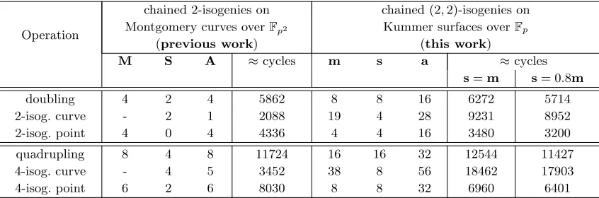
Efficiency of (2,2)-isogenies in SIDH. In Table 1, we compare (2,2)-isogenies on Kummer sur-faces with 2-isogenies on elliptic curves, by comparing the operation counts for isolated operations in both scenarios. On the elliptic curve side, the current state-of-the-art implementations actually use repeated 4-isogenies as they are slightly faster [16,14,27], so to take this into account we simply double the relevant operation counts for the (2,2)-isogenies reported above (recall from Lemma 2 that our (2,2)-isogenies correspond to 2-isogenies on the elliptic curves). Operation counts for the relevant 4-isogeny operations in the elliptic curve case are exactly as in the optimised version of the SIKE implementation [22], and for the relevant 2-isogeny operations are exactly as in [27, Table 1].
We use M, SandA to denote multiplications, squarings and additions inFp2, and use m, s
andato denote the same respective operations inFp. It is common to approximate the former in
terms of the latter by assuming Karatsuba-like routines forFp2 operations, but this can be rather
crude. To give a fairer comparison, we benchmarked these field operations directly using v3.0 of Microsoft’s SIDH library6: on a 3.4GHz Intel i7-6700 (Skylake) architecture, and over the 751-bit prime from [14], this benchmarking reportedM= 1004 cycles,S= 763 cycles, andA= 80 cycles, while m = 349 cycles and a = 43 cycles. The current library does not have a tailored squaring routine overFp, because the routines for Fp2 operations never call Fp squarings as a subroutine.
Thus, we give two cycle count approximations for the Kummer case: one that assumess=m(i.e., that theFpmultiplication routine is called to compute squarings), and one that assumess= 0.8m,
a common ratio used to approximate the speedup obtained by optimising tailored field squarings. We note that using cycle counts instead of Karatsuba approximations favours the elliptic curve setting over this work. For example, when using the above clock cycles as units, we haveM<3m, but a common approximation is thatM≈3m+ 5a3m.
The approximations in Table 1 suggest that the Kummer surface approach of computing Rich-elot isogenies overFpwill be competitive with the previous approaches that apply V´elu’s formulas
to the x-line of Montgomery elliptic curves over Fp2. The main operations of interest are
‘qua-drupling’ and ‘4-isog. point’, since these costs and their ratios are what determines the optimal strategy (see [16]), and they are computed many more times than the ‘4-isog. curve’ operation. Moreover, doubling the (2,2)-isogeny operation counts is only accurate in the case of the point operations; in terms of the curve operations, we would not need to compute the full set of the surface constants of the intermediate curve in back-to-back (2,2)-isogenies, so a more careful ap-proach to computing the image curve in this case would likely lead to counts close to half of those in this row (on our side). One caveat worth mentioning is that the special Kummer surfaces in this work will also have a fast ladder for computing scalar multiplications, as well as a fast three-point ladder that is typically used before any isogenies are computed in the SIDH framework.
6
Operation
chained 2-isogenies on chained (2,2)-isogenies on Montgomery curves overFp2 Kummer surfaces overFp
(previous work) (this work)
M S A ≈cycles m s a ≈cycles
s=m s= 0.8m
doubling 4 2 4 5862 8 8 16 6272 5714
2-isog. curve - 2 1 2088 19 4 28 9231 8952
2-isog. point 4 0 4 4336 4 4 16 3480 3200
quadrupling 8 4 8 11724 16 16 32 12544 11427
4-isog. curve - 4 5 3452 38 8 56 18462 17903
4-isog. point 6 2 6 8030 8 8 32 6960 6401
Table 1.Field arithmetic required for the three main isolated operations on one side of the SIDH frame-work, comparing chained 2-isogenies on Montgomery curves overFp2(previous work) with chained Richelot
isogenies on Kummer surfaces overFp(this work). Further explanation in text.
Of course, the only way to determine if the Kummer approach can outperform the elliptic curve approach is to present an optimised implementation of Kummer surface isogenies within the SIDH framework, e.g., one that factors in the cost ratios of pseudo-doublings and (2,2)-isogenies to derive optimal strategies for the full SIDH isogeny computation – see [16,§4.2]. We leave such an implementation as future work (perhaps until the motivation is heightened by odd-power Kummer isogenies that can be used on the other side of the SIDH protocol, as we discuss below), but also mention that Kummer arithmetic is especially amenable to aggressive vectorised implementations (see [5]).
Utilising Kummer surfaces in practice. We discuss two potential options for taking advantage of Kummer surface arithmetic in the SIDH framework, and the practical considerations of each. The first option is that the public parameters and wire transmissions are as usual, i.e., using (points on) elliptic curves, but that Kummer arithmetic is internally preferred by at least one party. The second assumes that Kummer arithmetic is preferred everywhere, and that the SIDH framework is defined to facilitate this.
Option 1 – Kummer arithmetic in private. Suppose Alice wants to compute her secret isogenies on Kummer surfaces while engaging in an SIDH protocol that is specified entirely using elliptic curves. In terms of the public parameters, her easiest option would be to convert them (offline and once-and-for-all) into Kummer parameters by first using the mapη:Eα→JCα in Section 3, and then applying the usual maps fromJCα to K
Sqr. While this process seems complicated at a first glance, a closer inspection of these maps reveals that an optimised conversion in this direction would only require a few dozen field multiplications; thex-coordinates of three co-linear points on Eα (see [14,22]) are all Alice needs to compute the corresponding Kummer surface and the three
Kummer points required to kick-start her computations. Indeed, the only additional information she needs to convert Bob’s public key down to the Kummer domain is the initial 2-torsion point (α,0) (assuming Bob sends her information for the curve coefficient instead), and this requires at most one square root inFp2, which is not a deal-breaker.
In the other direction, after computing her public key or shared secret on KSqr, Alice needs to lift this information back up toEα in order to comply with Bob. The maps lifting from KSqr
back up toJCλ,µ,ν are naturally more complicated than their inverses [19,13], but again the SIDH x-only framework simplifies the process significantly; we can recover thex-coordinate onEαgiven
In any case, equipped with the efficient maps in Section 3, we do not see any theoretical or practical obstacle preventing Alice from complying, should the efficiency of the Kummer warrant a small conversion overhead at either or both sides of the main isogeny computation.
Option 2 – Kummer arithmetic everywhere. If both sides of the SIDH protocol eventually warrant Kummer arithmetic (see below), then defining the public parameters to facilitate this is easy. The main issues we foresee involve maintaining the size of the public keys in the compressed setting.
Firstly, in the uncompressed scenario, transmitting elliptic curves and Kummer surfaces in the current framework has the same cost; Montgomery curves are specified up to twist with one element inFp2, and our supersingular Kummer surfaces are completely specified by two elements
of Fp (µ1 and µ2). Unambiguously specifying points on Montgomery curves amounts to sending one element of Fp2 and a sign bit; on the Kummer side, the elegant techniques in [28,§6] show
that Kummer points can be specified by two elements ofFp and two sign bits, meaning we lose at
most one bit per group element. Rather than sending any curve coefficients over the wire, recent works (including the SIKE proposal [22]) have instead specified public keys as three co-linear Montgomery x-coordinates, from which the underlying Montgomery curve can be recovered on the other side [14]. We have not yet investigated this analogue in the Kummer surface setting, but even if it does not work in a straightforward way, reverting back to the original form of public keys (from [16]) adds at most 4 bits to the public key sizes. To summarise, we would lose at most a few bits to specify uncompressed SIDH entirely using Kummer surfaces.
In terms of the shared secret, both parties would eventually arrive at a fast supersingular Kummer surface specified by (µ1: µ2: 1 : 1). While we have yet to investigate convenient Kummer surface invariants that could act as the shared secret, we remark that emperical evidence seems to suggest that the approach of computing λ, µ and ν = λµ from (15) and normalising the Igusa-Clebsch invariants inP(2,4,6,10)(Fp) makes the SIDH protocol commute. We leave further
investigation into appropriate invariants as future work.
In terms of optimal compression of public keys, applying the techniques in [2] directly to the Kummer setting seems less straightforward, but again we cannot see any reason preventing this possibility7. This too needs further investigation, but we point out that as a fallback, we could of course always map the problem of compression back to the elliptic curve setting (moving back to the first option above), and specify the compressed public keys accordingly.
Of course, there are several other possibilities that lie somewhere between the two options above, e.g., where the two parties send information in such a way that the overall cost of the protocol is minimised.
Beyond (2,2)-isogenies. The case for the Kummer approach in supersingular isogeny-based cryptography would be much stronger if it were able to be applied efficiently for both parties. There has been some explicit work done in the case of (3,3)- and (5,5)-isogenies (cf. [9,17]), but those situations appear much more complicated than the case of Richelot isogenies, and we leave their investigation as future work. One hope in this direction is the possibility of pushing odd degree`-isogeny maps from the elliptic curve setting to the Kummer setting by way of the maps in Section 3. This was difficult in the case of 2-isogenies because the maps themselves are (2, 2)-isogenies (e.g., their kernel is the 2-torsion onEα), but in the case of odd degree isogenies there
is nothing obvious preventing this approach.
References
1. R. Auer and J. Top. Legendre elliptic curves over finite fields.Journal of Number Theory, 95(2):303– 312, 2002.
2. R. Azarderakhsh, D. Jao, K. Kalach, B. Koziel, and C. Leonardi. Key compression for isogeny-based cryptosystems. In K. Emura, G. Hanaoka, and R. Zhang, editors,Proceedings of the 3rd ACM International Workshop on ASIA Public-Key Cryptography, AsiaPKC@AsiaCCS, Xi’an, China, May 30 - June 03, 2016, pages 1–10. ACM, 2016.
3. D. J. Bernstein. Curve25519: new Diffie-Hellman speed records. InInternational Workshop on Public Key Cryptography, pages 207–228. Springer, 2006.
4. D. J. Bernstein. Elliptic vs. Hyperelliptic, part I. Talk at ECC (slides athttp://cr.yp.to/talks/ 2006.09.20/slides.pdf), September 2006.
5. D. J. Bernstein, C. Chuengsatiansup, T. Lange, and P. Schwabe. Kummer strikes back: New DH speed records. In P. Sarkar and T. Iwata, editors,Advances in Cryptology - ASIACRYPT 2014 - 20th International Conference on the Theory and Application of Cryptology and Information Security, Kaoshiung, Taiwan, R.O.C., December 7-11, 2014. Proceedings, Part I, volume 8873 ofLecture Notes in Computer Science, pages 317–337. Springer, 2014.
6. D. J. Bernstein and T. Lange. Hyper-and-elliptic-curve cryptography. LMS Journal of Computation and Mathematics, 17(A):181–202, 2014.
7. J. W. Bos, C. Costello, H. Hisil, and K. E. Lauter. Fast cryptography in genus 2. J. Cryptology, 29(1):28–60, 2016.
8. J.-B. Bost and J.-F. Mestre. Moyenne arithm´etico-g´eom´etrique et p´eriodes des courbes de genre 1 et 2. Gaz. Math., 38:36–64, 1988.
9. N. Bruin, E. V. Flynn, and D. Testa. Descent via (3,3)-isogeny on Jacobians of genus 2 curves. Acta Arithmetica, 165:201–223, 2014.
10. J. W. S. Cassels and E. V. Flynn. Prolegomena to a middlebrow arithmetic of curves of genus 2, volume 230. Cambridge University Press, 1996.
11. A. M. Childs, D. Jao, and V. Soukharev. Constructing elliptic curve isogenies in quantum subexpo-nential time. J. Mathematical Cryptology, 8(1):1–29, 2014.
12. D. V. Chudnovsky and G. V. Chudnovsky. Sequences of numbers generated by addition in formal groups and new primality and factorization tests. Advances in Applied Mathematics, 7(4):385–434, 1986.
13. R. Cosset. Factorization with genus 2 curves. Math. Comput., 79(270):1191–1208, 2010.
14. C. Costello, P. Longa, and M. Naehrig. Efficient algorithms for supersingular isogeny Diffie-Hellman. In M. Robshaw and J. Katz, editors, Advances in Cryptology — CRYPTO 2016 — 36th Annual International Cryptology Conference, Santa Barbara, CA, USA, August 14-18, 2016, Proceedings, Part I, volume 9814 ofLecture Notes in Computer Science, pages 572–601. Springer, 2016.
15. A. Faz-Hern´andez, , J. L´opez, E. Ochoa-Jim´enez, and F. Rodr´ıguez-Henr´ıquez. A faster software implementation of the supersingular isogeny Diffie-Hellman key exchange protocol.IEEE Transactions on Computers, 67(11):1622–1636, 2017.
16. L. De Feo, D. Jao, and J. Plˆut. Towards quantum-resistant cryptosystems from supersingular elliptic curve isogenies. J. Mathematical Cryptology, 8(3):209–247, 2014.
17. E. V. Flynn. Descent via (5,5)-isogeny on Jacobians of genus 2 curves. Journal of Number Theory, 153:270–282, 2015.
18. S. D. Galbraith. Mathematics of public key cryptography. Cambridge University Press, 2012. 19. P. Gaudry. Fast genus 2 arithmetic based on Theta functions. J. Mathematical Cryptology, 1(3):243–
265, 2007.
20. H. Hisil and C. Costello. Jacobian coordinates on genus 2 curves. J. Cryptology, 30(2):572–600, 2017. 21. J. Igusa. Arithmetic variety of moduli for genus two. Annals of Mathematics, pages 612–649, 1960. 22. D. Jao, R. Azarderakhsh, M. Campagna, C. Costello, L. De Feo, B. Hess, A. Jalali, B. Koziel,
B. LaMacchia, P. Longa, M. Naehrig, J. Renes, V. Soukharev, and D. Urbanik. SIKE: Supersin-gular Isogeny Key Encapsulation. Manuscript available atsike.org/, 2017.
23. D. Jao and L. De Feo. Towards quantum-resistant cryptosystems from supersingular elliptic curve isogenies. In B. Yang, editor,Post-Quantum Cryptography - 4th International Workshop, PQCrypto 2011, Taipei, Taiwan, November 29 - December 2, 2011. Proceedings, volume 7071 of Lecture Notes in Computer Science, pages 19–34. Springer, 2011.
24. D. Lubicz and D. Robert. Arithmetic on abelian and Kummer varieties. Finite Fields and Their Applications, 39:130–158, 2016.
25. P. L. Montgomery. Speeding the Pollard and elliptic curve methods of factorization. Mathematics of computation, 48(177):243–264, 1987.
26. F. Oort. Subvarieties of moduli spaces. Inventiones mathematicae, 24(2):95–119, 1974.
![Fig. 1. An illustration of the two (2whendiagram in [28, Figure 1]. Here, 2)-isogenies corresponding to the subgroups Υ and Υ˜, based on the CΥ is used to denote CQ,P when P ∈ Υ, and C ˜Υ is used to indicate CQ,P P ∈ Υ˜.](https://thumb-us.123doks.com/thumbv2/123dok_us/7974856.1322417/17.612.117.492.293.397/illustration-whendiagram-figure-isogenies-corresponding-subgroups-denote-indicate.webp)