Extraction of Structural System Designs from Topologies via Morphological Analysis and Artificial Intelligence

(1)

Extraction of Structural System Designs from

Topologies via Morphological Analysis and Artificial

Intelligence

Achyuthan Jootoo1,†* and David Lattanzi2

1 _{PhD candidate, Department of Civil, Environmental, and Infrastructure Engineering, George Mason}

University, Fairfax, VA, USA, 22030; [email protected]

2 _{Assisstant Professor, Department of Civil, Environmental, and Infrastructure Engineering, George Mason}

University, Fairfax, VA, USA, 22030; [email protected] * Correspondence: [email protected]; Tel.: +1-571-447-2842

† Current address: Department of Civil, Environmental, and Infrastructure Engineering, George Mason University, Fairfax, VA, USA, 22030

Abstract:Structural system design is the process of giving form to a set of interconnected components 1

subjected to loads and design constraints while navigating a complex design space. While safe 2

designs are relatively easy to develop, optimal designs are not. Modern computational optimization 3

approaches employ population based metaheuristic algorithms to overcome challenges with the 4

system design optimization landscape. However, the choice of the initial population, or ground 5

structure, can have an outsized impact on the resulting optimization. This paper presents a new 6

method of generating such ground structures, using a combination of topology optimization (TO) 7

and a novel system extraction algorithm. Since TO generates monolithic structures, rather than 8

systems, its use for structural system design and optimization has been limited. In this paper, truss 9

systems are extracted from topologies through morphological analysis and artificial intelligence 10

techniques. This algorithm, and its assessment, constitutes the key contributions of this paper. The 11

structural systems obtained are compared with ground truth solutions to evaluate the performance 12

of the algorithms. The generated structures are also compared against benchmark designs from the 13

literature. The results indicate that the presented truss generation algorithm produces structures 14

comparable to those generated through metaheuristic optimization, while mitigating the need for 15

assumptions about initial ground structures. 16

Keywords:Structural Optimization; System Design; Artificial Intelligence; Morphological operations; 17

Topology Optimization; Structural Design. 18

1. Introduction 19

The conventional structural design process centers around the use of design requirements and 20

constraints to choose a single efficient structure from the large decision space of all possible designs, 21

all the while working with time and budget limitations. The structural design space has been shown to 22

be typically comprised of local optima, resulting in non-convex optimizations [1,2], and with solutions 23

often dependent upon specified initial conditions [3]. Compounding the problem, structures are 24

generally composed of a system of components, and so the performance and efficiency of any design 25

is governed by a combination of the system topology and the design of each component as well. Thus, 26

the design space for any set of design criteria can be extremely large. 27

Modern computational approaches for determining efficient structural designs often use a 28

metaheuristic, such as evolutionary computation, to obtain an optimal solution. Such metaheuristic 29

approaches are typically initialized via a ground structure approach, in which an assumed structural 30

system configuration serves as an initial sample population [4,5]. This paper presents a new method of 31

(2)

them, resulting in an optimal structure. [6] presented a method for discrete optimization of structural 37

assemblies using genetic algorithms. The structure was treated as a collection of nodes interconnected 38

via structural members. [7] used the ground structure approach for truss topology optimization. Similar 39

methods of structural optimization using the ground structure approach have been applied to diverse 40

problems [2–4] using various algorithms [5,8–11]. Further, with improved optimization heuristics and 41

higher computation capabilities, optimization has been performed for complex structures. However, 42

the key drawback to such approaches is that the final optimal design is dependent on the initial 43

structural systems selected for optimization [1,3] and a poorly chosen ground structure may lead to 44

suboptimal designs. 45

Topology optimization (TO), the process of finding the optimal layout (topology) of a structure, 46

requires fewer assumptions about the design domain compared to metaheuristic approaches. Two of 47

the most established TO approaches aredensity basedmethods andhard killmethods. Density based 48

methods discretize the design domain into a mesh and optimize the design by varying the density 49

of each element of the mesh based on an objective function. Fundamentally, this is a challenging 50

large-scale integer programming problem. In order to simplify the TO problem and express it as a 51

function of continuous design variables, an interpolation function with a penalization mechanism is 52

generally used. Different penalization and interpolation methods lead to different algorithms for TO 53

such as SIMP [12,13], Rational Approximation of Material Properties [14] and SINH [15]. A detailed 54

discussion of the SIMP approach, including implementation issues, can be found in [16]. For a review 55

of the recent developments in SIMP, the reader is referred to [17,18]. Research has also been conducted 56

in using TO with material failure constraints [19] and stress constraints [20]. TO has been widely 57

used in different domains such as fluid flow [21], heat transfer [22] and aerospace design [23,24]. 58

Hard kill methods gradually remove (or add) material from the design based on a heuristic strategy, 59

with Evolutionary Structural Optimization (ESO), developed by [25], as the most well known of such 60

methods. In this research, solid isotropic material with penalization (SIMP) was implemented due to its 61

widespread usage [17] and the chaotic convergence behavior of Evolutionary Structural Optimization 62

(ESO)[26]. 63

1.2. Contribution of this Research 64

As stated, a critical aspect of metaheuristic design optimization is the choice of ground structure 65

that serves as the initial population for optimization. Selecting such ground structures requires implicit 66

assumptions about the location of those structures in the design landscape. As such, there is a need 67

for methods to generate such structures automatically, without strong assumptions about the design 68

landscape. 69

Topology optimization presents an avenue for addressing this need. However regardless of the 70

specific method used, topology optimization results in monolithic structures, rather than the systems 71

of engineered components that comprise the majority of structural designs. This is a critical limitation, 72

as it inhibits topology optimization from being used to either generate initial structures for further 73

optimization, or for generating structural designs in many practical scenarios. 74

Presented in this paper is a new algorithm to generating structural systems, in the context of truss 75

design. This algorithm extracts structural systems from generated topologies, which can either be 76

analyzed directly or serve as the initial ground structures for further optimization. The extraction is 77

accomplished through a combination of morphological analysis and artificial intelligence techniques. 78

(3)

In this manuscript, the complete system extraction methodology is first presented. This is followed 80

by a study on the behavior of systems manually extracted from monolithic structural topologies. The 81

performance of three automatic extraction algorithm variants is then evaluated. A sensitivity study of 82

algorithm performance is included as well. 83

2. Methodology 84

The system generation process starts with a given design domain and the initial conditions 85

necessary to support topology optimization. A system topology is then generated through topology 86

optimization, based on these inputs (Section 2.1). Nodes and structural elements are extracted from this 87

topology through a combination of morphological analysis and associated computational techniques 88

(Section 2.2), yielding a structural assembly (system). The extracted structural assembly can then be 89

analyzed using FEA to perform structural analysis to obtain the deflections and member stresses. This 90

assembly can also serve as a basis for structural optimization. An overview of the process is provided 91

in Fig.1. 92

2.1. Topology Optimization 93

While any number of topology generation approaches can be used as part of the overall 94

methodology, in this work the SIMP density-method is used due to its consistent performance across a 95

range of application scenarios [26]. [27] first presented this approach for generating optimal topologies 96

in structural design using numerical optimization and homogenization methods. The objective of their 97

optimization was to minimize the work done by applied loads as shown in Eq.1. 98

In Eq. 1, Eijkl is the elasticity matrix,aE(u,v)is the energy in bilinear form i.e. the internal 99

virtual work of an elastic body at equilibriumuand for an arbitrary virtual displacementv,L(v) 100

represents the load linear form of the energy,fandtare body and boundary forces,eijrepresents the 101

linearized strain in each direction. Thus, this formulation minimizes the strain energy, while limiting 102

the displacements as per the imposed design constraints and the admissible displacements (U). 103

Minimize L(u)

subject toaE(u,v) =L(v); allv∈U, design constraints where

aE(u,v) = Z

ΩEijklekl(u)eij(v)dx,

eij(u) = 1 2(

∂ui ∂xj

+∂uj

∂xi ),

L(v) = Z

Ωf.vdx+

Z

Γt.vds

(1)

The design space of the problem is defined asΩ, the strain ase, and the indicator function 104

χ indicates whether material is present at a point x or not. Hence, for allx∈ Ω, eitherχ(x) =1 or 105

χ(x) =0 i.e. at any point in the domain, either material is present or it is not. This formulation also 106

assumes that the material is linearly elastic. For example, in Fig.1a, the black rectangle is the design 107

domain,Ω, with the black color throughout the design domain indicating thatχ(x) =1 everywhere. 108

As the design is optimized, the design domain remains the same but the location of material in the 109

domain changes, resulting in Fig. 1b. The elasticity matrix for the material is therefore defined as 110

Eijkl =χ(x)E0_ijklat any locationx. 111

This optimization problem can be modeled as a large scale integer programming problem and 112

is generally ill posed and difficult to solve [16]. [12] modified the problem by replacing the indicator 113

functionχ(x)with a density function,ρ(x), that is continuous between 0 and 1, rather than binary. 114

The modified elasticity matrix isEijkl=ρ(x)E0_ijkl. The density function transforms the problem from a 115

(4)

(5)

density value is either 0 or 1, constraints are imposed via penalization. This penalization supplies 117

the name of this approach: solid isotropic material with penalization (SIMP). The definition ofEijklis 118

further modified and it is redefined as: 119

Eijkl =ρ(x)pE0_ijkl, p>1 (2) Choosingp>1 makes the densities between 0 and 1 unfavorable since for the same amount of 120

material, it provides a lesser stiffness due to the exponentp. In general, in order to obtain solutions 121

with minimal volumes with intermediate densities, or binary designs, it is recommended to usep>=3. 122

Once the problem has been thus formulated, the density of the material within the design spaceΩis 123

optimized. The design at each iteration is analyzed through finite element analysis where each region 124

with a density value corresponds to an element. The value of the objective function is thus computed. 125

Based on the objective function, the topology is iteratively updated to yield a new topology until the 126

termination criteria are satisfied. 127

Since SIMP treats the topology optimization problem as essentially a material redistribution 128

problem, all resulting topologies are monolithic structures, rather than structural systems of 129

interconnected components. The second part of the presented computational process is designed to 130

extract such systems directly from the topologies. 131

2.2. Node-Element Extraction from Topologies 132

After a topology is obtained, the next step is to convert it into a system consisting of nodes (joints) 133

and connecting elements to suit structural engineering purposes. The morphological skeleton of the 134

topology, as well as branch and end points in that skeleton, are first found. The skeleton is then further 135

analyzed using one of the three variants of a node-element identification algorithm (NEI) developed in 136

this study (Fig.1). The first algorithm, NEI-CL (Section2.2.2), is based on clustering directional vectors 137

that initiate at a given a node and terminate at discretized locations throughout the topology. The 138

second algorithm, NEI-HLT (Section2.2.3), uses Hough transform line-finding to identify components 139

[28]. The third algorithm, NEI-TRA (Section2.2.4), is based on the concept of a structural component 140

as a path between nodes such that there is no other node along this path. Therefore, given the location 141

of nodes, this algorithm traverses from one node to another and identifies the connectivity between 142

nodes. 143

2.2.1. Topology skeletonization 144

The first step in identifying nodes and elements is to convert the generated topology into a 145

binarized and discretized representation, analogous to a black and white image. The binarization is 146

performed using Otsu’s method [29]. Theskeletonof the topology is then determined via morphological 147

thinning of the binarized topology [30]. The branch points and end points of the skeleton are detected 148

automatically by analyzing the 8-connectivity of the skeleton, yielding the potential nodes of the 149

structure. However, it is important to note that this method of identifying nodes does not necessarily 150

yield all of the correct nodes in some cases because of approximations in the skeletonization process. 151

Evidence of this effect will be shown in later analyses. 152

2.2.2. NEI-CL:Directional clustering algorithm variant 153

For the NEI-CL algorithm variant, the direction vectors from each node to each pixel in the 154

skeleton, within a specified distance from the node, are calculated. These vectors are clustered together 155

for each node using k-means clustering [31], with each cluster of vectors corresponding to a potential 156

structural element. Any two nodes with a clustered set of direction vectors oriented towards each other 157

are matched and identified as nodes and endpoints of a potential element. Structural elements are 158

then identified along each cluster’s direction vector, and the endpoints of these elements are labeled as 159

(6)

Figure 2.Pseudo code for the NEI-CL algorithm

Figure 3.Pseudo code for the NEI-HLT algorithm

This process occasionally results in multiple, and closely spaced, nodes at the ends of identified 161

elements. As a post-processing step, the set of nodes is clustered, again via the k-nearest neighbors 162

algorithm, to remove closely spaced and potentially duplicate nodes. Potential elements are also 163

evaluated for duplicates. Finally, all nodes without any connected elements are removed, yielding the 164

final set of nodes and elements. The pseudo code for this algorithm is shown in Fig.2. 165

2.2.3. NEI-HLT: Hough line transform based algorithm variant 166

As with the NEI-CL algorithm, the topology is first converted into a morphological skeleton, and 167

branch and endpoints are determined. The Hough transform [28,30], a well-established method for 168

finding line segments in images, is then applied. Given the assumption that all structural elements 169

will connect between nodes in a straight line, lines found through the Hough transform are labeled 170

as candidate structural elements. Duplicate endpoints of lines are merged using k-means clustering 171

and line segments with similar directionality and endpoints are joined to form a single element. The 172

pseudo code for this algorithm is shown in Fig.3. 173

2.2.4. NEI-TRA: Node to node traversal algorithm variant 174

The NEI-TRA algorithm variant iteratively traverses each segment initiating from each potential 175

node of the skeleton and stores the coordinates of each pixel in the traversal. The traversal, starting 176

from a node, proceeds by repeatedly moving from one pixel to another pixel in its 8 point neighborhood. 177

Once another identified node is reached and the traversal is complete, the goodness of fit of a line 178

connecting the two nodes is evaluated against the traversed pixels. The goodness of fit is evaluated 179

by using the coefficient of correlation and checking if all the traversed pixels fall within a specified 180

bandwidth from the line. If the fit is good, then an element is assigned between the two nodes. In 181

Fig.5a, the pixels from traversal along the segments 1, 2 and 3 have a good fit with the straight lines 182

connecting the nodes. If the fit is not good (Fig. 5a, segment 4), then the set of pixels is divided 183

into subsegments of the skeleton of a specified length (Fig. 5b) and the average direction vector is 184

computed for each subsegment. The direction vectors are then clustered so that subsegments with 185

similar direction vectors together are part of the same cluster. Subsegments in each cluster constitute 186

an element. Fig.5c shows a sample in which the subsegments have been clustered to yield elements. 187

If the endpoints of this element are not already present in the potential nodes, they are added as 188

additional nodes. Lastly, similar and duplicate nodes and elements are removed through k-means 189

clustering to obtain the final set of nodes and elements. The pseudo code for the NEI-TRA algorithm is 190

(7)

Figure 4.Pseudo code for the NEI-TRA algorithm

(8)

performed, as this variant produced the most consistent results. 198

3.1. Preliminary Analysis: Extracting Structural Systems from Topologies 199

In this study, the design constraints for two established problems from the structural optimization 200

literature were used as a basis for TO. Structural systems were then manually extracted from the 201

topologies, and the performance of these systems was compared against benchmark optimized 202

solutions from the literature. This study was performed in order to validate the initial idea of 203

generating structural systems using TO. The design problems shown in Fig.6a and7a were used as 204

input for TO, and extracted systems were compared with the results published by [4,10,32–34]. It is 205

important to clarify that the solutions in these previous works were obtained by starting from an initial 206

structural system, and iteratively optimized by adding members, removing members and, in some 207

cases, modifying node locations. These variations to the structure were introduced as per optimization 208

heuristics such as a genetic algorithm, particle swarm optimization, or differential evolution. 209

For the first design domain, “Problem 1”, a design space 18.288 meters (720 inches) wide and 9.144 210

meters (360 inches) high with two loads, each P = -444.82 kN (-100 kips), was specified. A design space 211

31.75 meters (1250 inches) wide and 6.35 meters (250 inches) high with 5 point loads, each P = -88.96 212

kN (-20 kips), acting on it was specified for “Problem 2”. Loads and boundary conditions were applied 213

as per Fig.6a and7a. Topologies were generated using a modified version of Sigmund’s 99 line Matlab 214

code for SIMP [35]. Each structure was converted to a truss system by manually identifying nodes and 215

elements, and adding extra members if needed for stability. The results obtained were then imported 216

into [36] for evaluation. The designs reported in the literature were also evaluated in Risa 2D. 217

SIMP requires a volume fraction parameter, a parameter that determines the fraction of the 218

volume of the design domain that will contain material. Several volume fractions were tested and 219

it was observed that higher volume fractions increased the weight of the structure and reduced the 220

deflections and member stresses, as is to be expected. For both problems, a volume fraction was 221

eventually selected that generated design weights comparable to prior efforts. Since the objective 222

function of SIMP topology optimization is evaluated via finite element analysis, parameters for 223

discretization of the design domain such as the number of elements needs to be specified. The impact 224

of the fineness of the discretization has been well documented in the TO literature [16], and is not 225

studied here. The mesh resolutions chosen here were 60x30 for Problem 1 and 175x35 for Problem 2 226

because changing the discretization around these resolutions the did not impact the TO result. 227

3.1.1. Metrics 228

As the the volume fraction was iteratively changed to match previous design weights, the 229

structural weight was not useful as a comparative metric. Instead, the average stress, maximum stress, 230

and maximum deflection were used for comparisons. 231

3.1.2. Results 232

For Problem 1, the volume ratio was specified as 0.2. With regards to the compared studies, [32] 233

and [4] only varied the cross-sectional area of the initial structure but did not add or remove members. 234

[10] presented a solution with no removal of members and another solution in which removal of 235

structural members was permitted. A comparison of the weight, deflection, maximum stress and 236

(9)

Figure 6.(a)Initial structure for prior solutions to Problem 1 [10], (b) optimal solution from [10], and (c) TO solution, and (d) TO solution converted to a truss

Table 1.Comparative results for Problem 1

Perez and Xu et al. Wu and Wu and TO System

Metrics Behdinan (2009) Tseng Tseng

(2007) (2010)∗ (2010)∗∗

Weight (kgs) 2278.94 2303.45 2295.38 2145.80 2323.07

Deflection (cm) 5.11 5.08 5.05 5.08 5.21

Maximum Stress (MPa) 172.51 140.65 172.37 128.93 57.98

Average Stress (MPa) 56.54 49.64 56.54 74.26 49.78

* Results without member removal ** Results with member removal

The structure optimized by [10], which permitted member removal, was 5.8% lighter than the 238

other structures, which all had very similar weights. The TO-based truss was the heaviest, and had 239

slightly higher deflections. The TO-based results reflect a maximum stress of 58.0 MPa and an average 240

stress of 49.8 MPa, which is a notably more even stress distribution than the other structures. It is 241

assumed that, given additional optimization, the TO-based system would converge to a solution 242

similar to those of prior efforts. 243

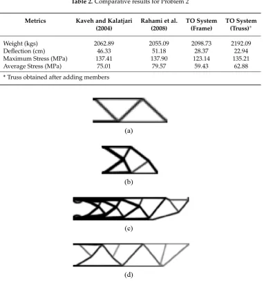
The TO solution to Problem 2 was compared with the designs published in [33,34]. In both of 244

these studies, an initial structure was assumed for optimization. The node locations could be modified, 245

but member removal was not permissible. The area of cross-section of the members could also be 246

modified to optimize the structure. For the topology optimization, the volume ratio was set to 0.2. 247

TO resulted in structures that were unstable when directly converted to trusses, a problem not 248

encountered in Problem 1. Hence, the structure was first evaluated as a frame with complete joint 249

fixity. Members were then manually added to this frame for stability, and it was converted to a truss 250

with pin supports (Fig.7d). A comparison of the results is shown in Table2. 251

Table2shows that the structures optimized in the literature are lighter than the TO designed 252

structures by about 2% for the frame structure and 6.7% for the truss structure. However, the TO 253

structure has slightly lower maximum stresses, lesser average stress and significantly lower deflections. 254

(10)

Figure 7.(a)Initial structure for prior solutions to Problem 2, (b) optimal solution from [34], (c) TO solution, and (d) TO solution converted to truss. Note the additional members needed for stability

[33] and [34]. Also, the variation in the member stresses is 13.6% lesser for the TO truss structure and 256

33.6% lesser for the TO frame structure, which indicates a more evenly distributed load in the TO 257

structure. This is similar to the results of Problem 1. 258

What the results of this analysis illustrate is that systems extracted from structural topologies 259

can perform comparably to systems optimized assuming an initial structural configuration. This is 260

particularly true given that the extracted systems could be further optimized using any number of 261

established techniques. Therefore, generating a topology and then extracting a system from it can serve 262

as a full replacement for an initial estimate of a structural configuration. In such cases, the specified 263

volume ratio becomes the controlling design parameter. It is also important to recognize that, as shown 264

by Problem 2, topology optimization results can require some post-processing in order to generate 265

stable results. 266

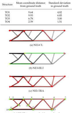
3.2. Extraction Algorithm Analysis 267

In the preliminary analysis, systems were manually extracted from topologies. The three automatic 268

extraction algorithms designed to address this issue are analyzed in this section. Four diverse 269

topologies (TO1, TO2, TO3, TO4) were generated and used for testing (Fig. 8). These topologies 270

have variations in member thickness, number of members, and general topological complexities that 271

illustrate both the capabilities and limitations of the extraction process. A ground truth extraction 272

solution was developed based on manual labeling of nodes and elements in the TO structure. After 273

evaluating the three variants, a parameter sensitivity analysis was conducted for NEI-TRA, as it 274

(11)

Table 2.Comparative results for Problem 2

Metrics Kaveh and Kalatjari Rahami et al. TO System TO System

(2004) (2008) (Frame) (Truss)∗

Weight (kgs) 2062.89 2055.09 2098.73 2192.09

Deflection (cm) 46.33 51.18 28.37 22.94

Maximum Stress (MPa) 137.41 137.90 123.14 135.21

Average Stress (MPa) 75.01 79.57 59.43 62.88

* Truss obtained after adding members

Figure 8.TO structures used as inputs for algorithm to identify nodes and elements

3.2.1. Metrics 276

Fundamentally, the performance of each algorithm was evaluated based on how accurately it 277

identified nodes and elements. Since the nodes in a TO structure are not visually distinct as a single 278

point but as a region, identifying the exact ground truth node location is subjective. In order to 279

capture this subjectivity, and to determine the most likely node location, the labeling of the nodes 280

was performed by twenty individuals. The marked locations were then averaged to yield the ground 281

truth. A standard deviation indicating the variation in individual marking of node locations was also 282

computed (termed as "node location variance"). This node location variance quantified the subjectivity 283

of the node identification in the ground truth itself and, as will be shown, correlated with the ability of 284

the extraction algorithms to properly segment the structures. The node location variance is illustrated 285

as green circles (radius is proportional to the variance) in Fig.9d,10d,11d and12d. 286

3.2.2. Results 287

The results for TO1 are shown in Fig. 9. A visual examination clearly shows that the traversal 288

based algorithm (NEI-TRA) outperforms the other two algorithms. As shown in Table3the cluster 289

(12)

Figure 9.Node and element identification results for TO1

Table 3.Number of nodes and elements identified by different algorithms

Structure Number of Nodes Identified Number of Elements Identified

GT NEI-CL NEI-HLT NEI-TRA GT NEI-CL NEI-HLT NEI-TRA

TO1 7 6 4 10 10 7 2 13

TO2 6 4 2 7 7 4 1 8

TO3 16 5 7 19 26 5 5 29

TO4 13 6 4 13 19 6 2 19

GT: ground truth result

transform based algorithm (NEI-HLT) only identified two elements out of a total of ten elements (Fig. 291

9b). The reason for this poor performance is that the hough line transform uses the skeleton to identify 292

straight segments. Approximations in the skeleton in the form of curves result in the hough transform 293

being unable to detect lines. Hence, in skeletons obtained from poorly defined or curved topologies, 294

the performance of the hough line transform is poor. With regards to NEI-TRA (Fig. 9c), there is a 295

slight oversegmentation of one element and it thus identifies 13 elements instead of 10. 296

Multiple nodes were identified at some joints since the analysis of the morphological skeleton 297

(Fig.9e) occasionally yielded closely spaced branch points. It is worth noting that 40% of the manually 298

grount truth sets indicated two nodes as well, similar to what the algorithm indicated. For the nodes 299

with more node location variance in the ground truth (1, 6, 8 and 9), the algorithm results were a little 300

farther from the ground truth. The NEI-TRA algorithm detected all the elements of the structure. 301

The performance of the three algorithms for TO2 is shown in Fig.10and Table3. The NEI-CL 302

algorithm detected all but two elements and identified a majority of the nodes in the structure. The 303

(13)

skeletonization. The NEI-TRA algorithm identified all the elements and nodes. However, due to the 305

skeleton’s structure, additional nodes were detected as seen with TO1. 306

A comparison with the ground truth (Fig.10d) showed that the performance of the NEI-TRA 307

algorithm was superior. It identified the nodes accurately in all cases. Multiple nodes along with an 308

extra element were detected at two joints in the structure due to the skeleton having multiple branch 309

points in the vicinity of that joint. The algorithm correctly detected only one node in the top left corner 310

whereas 50% of the ground truth labels had two nodes at this joint. 311

The nodes and elements identified by each of the algorithms for TO3 are shown in Fig.11. The 312

NEI-TRA algorithm outperforms the other two variants in this case as well. The NEI-CL algorithm 313

performed relatively poorly due to the increased amount of material in this structure (as a result 314

of a higher volume ratio). The algorithm erroneously identified elements which do not exist as a 315

result. The NEI-HLT algorithm also performed poorly, with only a few elements being detected due to 316

approximations in the skeleton. The NEI-TRA algorithm provided the most reasonable system again 317

with a slight oversegmentation. 318

Comparing with the ground truth, the NEI-TRA algorithm again shows multiple nodes at some 319

joints (Fig.11d) due to the skeleton containing multiple branch points in those locations. Nodes with 320

more variance in the ground truth labeling, such as nodes 2 and 12, had more distance between the 321

ground truth node and algorithm identified node (see Table4). In contrast, node 13 is accurately 322

identified although the variance in the ground truth was high for this node. It is worth noting that 323

noticeable errors were obtained at the leftmost nodes of the structure (nodes 1 and 11) since the skeleton 324

endpoint is not exactly at the actual structure support location. 325

Fig.12shows the nodes and elements identified by the three algorithms for TO4 structure. The 326

results show that the NEI-TRA algorithm was again the best performer. The NEI-HLT algorithm 327

(14)

Table 4.Evaluating the NEI-TRA algorithm performance against the ground truth node coordinates

Node # Ground truth coordinates

Distance from ground truth

Variance in ground truth

1 (74.8,165) 12.1 2.68

2 (130,167) 22.2 5.46

3 (182,168) 7.28 3.13

4 (252,165) 8.97 2.88

7 (505,169) 3.61 2.41

10 (319,194) 0.83 1.81

11 (74.8,241) 11.7 3.07

12 (125,236) 13.1 5.01

(15)

Table 5.Geometric accuracy of the NEI-TRA algorithm

Structure Mean coordinate distance from ground truth

Standard deviation in ground truth

TO1 9.64 4.82

TO2 9.93 6.85

TO3 6.78 3.00

TO4 2.59 1.51

about half of the elements in the structure. The nodes detected were however very close to the actual 329

node locations from the benchmark solutions. 330

Since this topology’s elements have less thickness, the skeleton of the structure is a very good 331

representation of the actual structure. As a result, the NEI-TRA algorithm detects nodes and elements 332

very accurately. Quantitatively, it can be seen that the mean error in node location for TO4 was much 333

lower than the node location error for all other structures tested (Table5). Hence, the solution obtained 334

using the traversal based algorithm is very close to the ground truth solution (Fig.12d). 335

3.2.3. Summary 336

This analysis showed that the NEI-TRA algorithm, based on depth first search traversal and 337

k-means clustering, clearly demonstrated superior performance compared to the NEI-CL and NEI-HLT 338

algorithms. NEI-HLT performs poorly due to approximations in skeletonization. NEI-CL erroneously 339

identifies direction vector clusters as elements leading to falsely identified elements. This erroneous 340

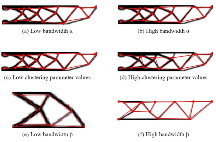
identification of clusters is a classic problem of separating signal (clusters that are actual elements) from 341

(16)

The NEI-TRA algorithm has five controlling parameters. A bandwidth parameter, “α”, is used 348

to check if the line connecting two nodes is a good fit for the pixels (Fig.4, line 8). Three additional 349

parameters are used for clustering nodes in order to eliminate similar nodes (Fig. 4, line 17), and a 350

second bandwidth parameter “β” is used for removing redundant elements and breaking up long 351

elements into smaller elements if the required criteria are met (Fig. 4, line 17). The effect of each 352

parameter is explored in greater depth in this section. 353

3.3.1. Impact of bandwidth parameterα

354

6 different values of the bandwidth parameterα, from 2 pixels to 12 pixels, were tested. In the 355

results shown, anα value of 4 was used. It was observed that the impact of this parameter on the 356

resulting system is not significant since the main purpose of this parameter is to make the algorithm 357

faster. Once the pixels from the traversal are determined, there are two ways of processing it. If the line 358

connecting the end point nodes is a good fit, which is true if no pixel is more thanα pixels away from 359

a line, then an element connecting the nodes is added (Fig.4, line 15-16). If the fit is not good, then a 360

clustering approach is used (Fig.4, line 9-14). Ifα is too small, then the clustering approach is used 361

more frequently resulting in a slower runtime. Further, the clustering approach can determine different 362

endpoints from the existing nodes and hence create additional nodes. However, after removing similar 363

nodes, the final nodes and elements obtained did not change significantly as seen for TO3 (Fig.13c). 364

3.3.2. Impact of the three clustering parameters 365

In order to remove redundant nodes, clustering is used (Fig.4, line 17). Three parameters together 366

control this clustering. 15 combinations of these parameters, with settings varying from 5 pixels to 367

30 pixels, were evaluated. Small values for these parameters cluster only the nodes which are very 368

close to each other whereas larger values can cluster nodes which are farther apart spatially. This 369

can be seen in Fig.13f where higher values of these parameters cluster nearby nodes. For TO3, the 370

impact was most noticeable since nodes are relatively close to each other. Hence, higher values of this 371

parameter ended up clustering non redundant nodes which should not be clustered into one node. 372

The best results were obtained with the three parameters having values of 10, 15 and 7.5. 373

3.3.3. Impact of bandwidth parameterβ

374

Redundant elements are removed and long elements are broken into appropriate smaller elements 375

using the control parameterβ. For example, the top elements in Fig.13h, which connect the leftmost 376

top node to the rightmost top node are formed by breaking a long element that connects the leftmost 377

and rightmost nodes into multiple smaller elements with intermediate nodes. 10β values ranging 378

from 5 pixels to 50 pixels were tested for this sensitivity analysis. If the value of the parameter was 379

too large (more than 40 pixels), then the element was erroneously segmented as shown in Fig.13h. 380

Similarly erroneous segmentations were seen in the other topologies as well. If the parameter was too 381

small (10 pixels or less), then some redundancy in elements persisted as illustrated for TO1 in Fig.13g. 382

Aβ value of 20 resulted in the most consistent element identification. 383

4. Conclusions and Future Work 384

This paper presents a new method of generating structural systems using a combination of 385

(17)

Figure 13.Impact of different parameters on the performance of the NEI-TRA algorithm

benefits of this approach are that, compared to other approaches to structural optimization, it does 387

not require an assumed structural system for initiation. Instead, broader constraints such as loadings, 388

geometric boundaries, and volume ratios are required instead. 389

From the preliminary TO system study, several conclusions can be drawn. One of the foremost 390

observations is that structural systems derived manually through TO are efficient and comparable 391

to optimal structures from the literature in most cases. These systems were comparable with respect 392

to deflections. The TO-based systems resulted in more balanced member stresses compared to the 393

benchmark solutions, which had members with very high and very low stresses. In some cases, 394

however, the system extracted from the topology was not stable for a truss configuration, requiring 395

manual post-processing. 396

Once the viability of using TO for deriving systems was verified, the three extraction algorithms 397

were tested. The NEI-TRA algorithm demonstrated the most consistent performance and accurately 398

identified the most nodes and elements across different scenarios. A key aspect of the extraction 399

process presented here is the analysis of the morphological skeleton to identify nodes and their 400

connectivity. Hence, the algorithm performs well in scenarios where the skeleton of the structure is a 401

close representation of the actual structure. In situations where this does not hold, the performance 402

of the algorithm deteriorates. This was clearly seen in cases where the skeletonization process was 403

modified to yield a skeleton unrepresentative of the actual structure. The algorithm itself is dependent 404

on several parameters. The best performance was seen when the values of the bandwidthα was 4, 405

β was 20 and the three clustering parameter values were between 7.5 and 15. The values of these 406

parameters will change depending on the scale of the input for the algorithms. Higher resolution 407

inputs to the algorithm will need larger parameter values and vice versa. 408

One persistent issue with the NEI-TRA algorithm was the multi-node problem wherein multiple 409

nodes were detected instead of a single node. Further research is required to remedy this issue. 410

Another avenue for future work is to use additional structural optimization to further improve the 411

designs generated through the topology extraction process. 412

Author Contributions: Achyuthan Jootoo and David Lattanzi conceived and designed the experiments. 413

Achyuthan Jootoo developed the algorithms and programs, performed the experiments, and analyzed the 414

data. Achyuthan Jootoo wrote the paper with reviews, significant inputs and edits by David Lattanzi. 415

(18)

NEI-HLT: Node element identification via Hough Line Transform 423

NEI-TRA: Node element identification via node to node Traversal 424

425

1. Rajan, S.D. Sizing, Shape, and Topology Design Optimization of Trusses Using Genetic Algorithm.Journal 426

of Structural Engineering1995,121, 1480–1487. 427

2. Ho-Huu, V.; Vo-Duy, T.; Luu-Van, T.; Le-Anh, L.; Nguyen-Thoi, T. Optimal design of truss structures with 428

frequency constraints using improved differential evolution algorithm based on an adaptive mutation 429

scheme.Automation in Construction2016,68, 81–94. 430

3. Kicinger, R.; Arciszewski, T.; DeJong, K. Evolutionary Design of Steel Structures in Tall Buildings. Journal 431

of Computing in Civil Engineering2005,19, 223–238. Similar to the Murawski (2000) paper; experiments and 432

results; not much theory;. 433

4. Xu, T.; Zuo, W.; Xu, T.; Song, G.; Li, R. An adaptive reanalysis method for genetic algorithm with 434

application to fast truss optimization. Acta Mech Sin2009,26, 225–234. 435

5. Tejani, G.G.; Savsani, V.J.; Bureerat, S.; Patel, V.K. Topology and Size Optimization of Trusses with Static 436

and Dynamic Bounds by Modified Symbiotic Organisms Search.Journal of Computing in Civil Engineering 437

2017,32, 04017085. 438

6. Rajeev, S.; Krishnamoorthy, C. Discrete Optimization of Structures Using Genetic Algorithms. J. Struct. 439

Eng.1992,118, 1233–1250. Insights into the GA setup and working. 440

7. Hajela, P.; Lee, E. Genetic algorithms in truss topological optimization.International Journal of Solids and 441

Structures1995,32, 3341–3357. 442

8. Gandomi, A.H.; Yang, X.S.; Alavi, A.H. Mixed variable structural optimization using Firefly Algorithm. 443

Computers & Structures2011,89, 2325–2336. 444

9. Hasancebi, O.; Azad, S.K. Adaptive dimensional search: A new metaheuristic algorithm for discrete truss 445

sizing optimization.Computers & Structures2015,154, 1–16. 446

10. Wu, C.Y.; Tseng, K.Y. Truss structure optimization using adaptive multi-population differential evolution. 447

Struct Multidisc Optim2010,42, 575–590. 448

11. Goncalves, M.S.; Lopez, R.H.; Miguel, L.F. Search group algorithm: A new metaheuristic method for the 449

optimization of truss structures. Computers and Structures2015,153, 165–184. 450

12. Bendsoe, M.P. Optimal shape design as a material distribution problem. Struct Multidisc Optim1989, 451

1(4), 193–202. 452

13. Zhou, M.; Rozvany, G.I.N. The COC algorithm, Part II: Topological, geometrical and generalized shape 453

optimization.Computer Methods in Applied Mechanics and Engineering1991,89, 309–336. 454

14. Stolpe, M.; Svanberg, K. An alternative interpolation scheme for minimum compliance topology 455

optimization.Struct Multidisc Optim2001,22, 116–124. 456

15. Bruns, T.E. A reevaluation of the SIMP method with filtering and an alternative formulation for solid–void 457

topology optimization.Struct Multidisc Optim2005,30, 428–436. 458

16. Bendsoe, M.P.; Sigmund, O. Topology optimization: theory, methods, and applications; Springer Science & 459

Business Media, 2013. 460

17. Deaton, J.D.; Grandhi, R.V. A survey of structural and multidisciplinary continuum topology optimization: 461

post 2000.Struct Multidisc Optim2013,49, 1–38. 462

18. Sigmund, O.; Maute, K. Topology optimization approaches. Struct Multidisc Optim2013,48, 1031–1055. 463

19. Pereira, J.T.; Fancello, E.A.; Barcellos, C.S. Topology optimization of continuum structures with material 464

failure constraints. Struct Multidisc Optim2004,26, 50–66. 465

20. Bruggi, M.; Duysinx, P. Topology optimization for minimum weight with compliance and stress constraints. 466

(19)

21. Kreissl, S.; Pingen, G.; Maute, K. Topology optimization for unsteady flow. Int. J. Numer. Meth. Engng. 468

2011,87, 1229–1253. 469

22. Zhou, S.; Li, Q. Computational design of multi-phase microstructural materials for extremal conductivity. 470

Computational Materials Science2008,43, 549–564. 471

23. Wang, Q.; Lu, Z.; Zhou, C. New Topology Optimization Method for Wing Leading-Edge Ribs.Journal of 472

Aircraft2011,48, 1741–1748. 473

24. Zhu, J.H.; Zhang, W.H.; Xia, L. Topology Optimization in Aircraft and Aerospace Structures Design. 474

Archives of Computational Methods in Engineering2016,23, 595–622. 475

25. Xie, Y.M.; Steven, G.P. A simple evolutionary procedure for structural optimization. Computers & structures 476

1993,49, 885–896. 477

26. Rozvany, G.I.N. A critical review of established methods of structural topology optimization. Struct 478

Multidisc Optim2008,37, 217–237. 479

27. Bendsoe, M.P.; Kikuchi, N. Generating optimal topologies in structural design using a homogenization 480

method. Computer Methods in Applied Mechanics and Engineering1988,71, 197–224. 481

28. Duda, R.O.; Hart, P.E. Use of the Hough Transformation to Detect Lines and Curves in Pictures. Commun. 482

ACM1972,15, 11–15. 483

29. Otsu, N. A threshold selection method from gray-level histograms.IEEE transactions on systems, man, and 484

cybernetics1979,9, 62–66. 485

30. Gonzalez, R.C.; Woods, R.E.Digital Image Processing; Pearson, 2007. 486

31. Witten, I.; Frank, E.; Hall, M.Data Mining: Practical Machine Learning Tools and Techniques, 3rd ed.; Morgan 487

Kaufmann: Burlington, MA, 2011. 488

32. Perez, R.E.; Behdinan, K. Particle swarm approach for structural design optimization. Computers & 489

Structures2007,85, 1579–1588. 490

33. Kaveh, A.; Kalatjari, V. Size/geometry optimization of trusses by the force method and genetic algorithm. 491

Z. angew. Math. Mech.2004,84, 347–357. 492

34. Rahami, H.; Kaveh, A.; Gholipour, Y. Sizing, geometry and topology optimization of trusses via force 493

method and genetic algorithm.Engineering Structures2008,30, 2360–2369. 494

35. Sigmund, O. A 99 line topology optimization code written in Matlab. Struct Multidisc Optim2001, 495

21, 120–127. 496