Evaluation of Machine Learning Techniques for Daily Reference Evapotranspiration Estimation
Ali Rashid Niaghi1*, Oveis Hassanijalilian1,Jalal Shiri2
1. Agricultural and Biosystems Engineering Department, Ph.D. Candidate, North Dakota State
University, Fargo, ND. Email: [email protected].
2. Water Engineering Department, Faculty of Agriculture, University of Tabriz, Tabriz, Iran.
Abstract
The ASCE-EWRI reference evapotranspiration (ETo) equation is recommended as a standardized
method for reference crop ETo estimation. However, various climate data as input variables to
the standardized ETo method are considered limiting factors in most cases and restrict the ETo
estimation. This paper assessed the potential of different machine learning (ML) models for ETo
estimation using limited meteorological data. The ML models used to estimate daily ETo
included Gene Expression Programming (GEP), Support Vector Machine (SVM), Multiple
Linear Regression (LR), and Random Forest (RF). Three input combinations of daily maximum
and minimum temperature (Tmax and Tmin), wind speed (W) with Tmax and Tmin, and solar
radiation (Rs) with Tmax and Tmin were considered using meteorological data during 2003–2016 from six weather stations in the Red River Valley. To understand the performance of the applied
models with the various combinations, station, and yearly based tests were assessed with local
and spatial approaches. Considering the local and spatial approaches analysis, the LR and RF
models illustrated the lowest rate of improvement compared to GEP and SVM. The spatial RF
and SVM approaches showed the lowest and highest values of the scatter index as 0.333 and
0.457, respectively. As a result, the radiation-based combination and the RF model showed the
best performance with higher accuracy for all stations either locally or spatially, and the spatial
SVM and GEP illustrated the lowest performance among models and approaches.
1 Introduction
Evapotranspiration (ET) is a combination of two separate processes that transfers huge volumes
of water and energy from the soil (evaporation) and vegetation (transpiration) to the atmosphere
[1,2]. Since ET plays a crucial rule in watershed and agricultural water management, accurate
spatial and temporal estimation crop water requirements (ETa) at the scale of human influence is
a critical need for a wide range of applications [3]. Quantifying ETa from agricultural lands is
vital to management of water resources. Measurement methods of ETa are available through
water vapor transfer methods (e.g. Bowen ratio, eddy covariance) [4–6], water budget
measurements (e.g. soil water balance, weighting lysimeters) [7–9], or remote sensing techniques
[10–12]. However, the application of field scale methods is limited due to the cost, complexity
and maintenance. Estimating ETa using remote sensing models has developed in the recent years
but cloud existence in many areas during the satellite passing dates limits the ability of imagery
usefulness. Therefore, due to difficulties of ETa direct measurements, ETa can be estimated using
by multiplying the calculated reference ET (ETo), using different calculation methods and
meteorological data, with the crop coefficient (Kc). However, required meteorological data for
ETo calculation methods are not readily available for many locations, and methods with fewer
variables must be considered when basic meteorological data are available [13]. However, the
simplified and basic models are suited to estimate ETo on a weekly or monthly basis instead of
daily basis [14].
The ETo calculation is a complex process due to the large number of associated
meteorological variables, and it is hard to develop an accurate empirical model to overcome all
complexity of the process. Over the last decades, machine learning (ML) techniques have
estimation complexity. These methods are evolutionary computation techniques that can achieve
the best relationship in a system with data driving tool. Due to the capability of the ML methods
in tackling non-linear relationship between dependent and independent variables [15], numerous
ML techniques have been applied and proposed to predict ETo for agricultural purposes
including genetic programming (GP) [16,17], kernel based algorithms, e,g, support vector
machine (SVM) [18,19], artificial neural network [20–22], wavelet neural network [13,23],
random forest (RF) [24,25], and multiple linear regression (LR) [26,27].
Several authors have applied ML methods to detect ETo values with minimum variation from
observed values [15,20,28]. Among these models, the GEP and SVM illustrated better estimation
than other models [19,29]. The Gene Expression Programming (GEP) is comparable to GP and
both involve different size and shapes of computer programs encoded in linear chromosomes of
fixed length [16]. The SVM method is a regression procedure that has been used successfully in
hydrology context [30–32] and agro-hydrology for ETo modelling [18,33]. GEP has several
advantages compared to GP such as generating valid structure, multigenic nature, and ability of
surpasses the old GP system. Shiri et al. [16] evaluated GEP to estimate daily evaporation
through spatial and temporal data scanning. Shiri and Kişi [34] compared the GEP and Adaptive
neuro-fuzzy inference system (ANFIS) techniques for predicting short and long-term river flows.
Also, Shiri and Kişi [34] used a similar comparison to predict groundwater table fluctuations.
Kişi and Çimen [33] studied the potential of SVM model in ETo prediction and observed that the
SVM model could be useful for ETo estimation and hydrological modeling studies.
The LR model is one of the commonly used ML methods in hydrology [27,35]. It has been
used to cover the study of the relationship between two or more hydrological variables and
Some researchers have used the LR method to estimate the ETo rate for different regions due to
the simplicity of the method compared to other numerical methods [36,37]. Tabari et al.
[26]compared the LR and SVM model’s performance for semi-arid region and found that SVM
model was superior to empirical and LR models.
Due to the high computational costs and complexity of the ML models, the tree-based
ensemble models attract people by its simplicity and estimation power. The RF model as a ML
tree-based model is able to produce a great result compared to the other ML models [24,38]. This
model known for its simplicity and the ability for both classification and regression tasks. The
RF method is also widely used to predict the ET rate of different climate regions [39]. Feng et al.
[25] applied RF model for ETo estimation on a daily basis for southwest China and indicated that
the RF model performed slightly better than the GRNN model. Shiri [40] evaluated the coupled
RF with wavelet algorithm to estimate ETo for southern part of Iran and obtained that the
coupled RF model showed great improvement compared to the conventional RF and empirical
models. And to our knowledge, this model has not been applied in the Northern US for ETo
studies.
According to the literatures, GEP and SVM models have been frequently applied among the
world for various climate conditions for ETo estimation, while the LR and RF model’s
application were minimal. In addition, these models have not been compared with commonly
used SVM and GEP models for sub-humid climate condition. Since the limited studies have been
conducted to evaluate ML models for Northern part of the US (that experiences a high variability
of weather conditions and a huge amount of agricultural production), the objectives of this study
were to investigate the effect of different input combination of meteorological data on the
2) compare the spatial and temporal prediction capabilities of the different ML models in ETo
estimation, and 3) evaluate the performance of the models based on the various study years and
meteorological station.
2 Materials and Methods
2.1 Study area climate and reference evapotranspiration (ETo)
The weather data for current study were obtained from the North Dakota Agricultural Weather
Stations [41] located at the Prosper (ND), Galesburg (ND), Leonard (ND), Sabin (MN), Perley
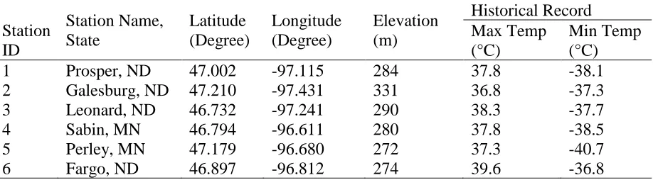
(MN), and Fargo (ND) for 17 years (January 2003-December 2016) (Table 1).
Table 1 Study weather data locations measured at the NDAWN automated stations Station Name, State Latitude (Degree) Longitude (Degree) Elevation (m) Historical Record Station ID Max Temp (°C) Min Temp (°C)
1 Prosper, ND 47.002 -97.115 284 37.8 -38.1
2 Galesburg, ND 47.210 -97.431 331 36.8 -37.3
3 Leonard, ND 46.732 -97.241 290 38.3 -37.7
4 Sabin, MN 46.794 -96.611 280 37.8 -38.5
5 Perley, MN 47.179 -96.680 272 37.3 -40.7
6 Fargo, ND 46.897 -96.812 274 39.6 -36.8
Table 2 shows the statistical analysis of the weather data for the study stations during the study
period.
Table 2 Daily statistical parameters of the applied data
station parameter unit Xmax Xmin Xmean SX CV CSX
Prosper,
ND
Tmax °C 37.9 24.3 11.3 14.3 1.27 -0.37
Tmin °C -29.8 -38.1 -0.8 13.0 -16.73 -0.28
WS m s-1 14.2 0.9 4.2 1.8 0.43 0.55
Rh % 100 13.8 68.6 15.6 0.23 -0.14
RS MJ m-2 31.1 0.3 13.2 7.9 0.60 0.51
ETo mm 11.4 0 2.4 2.03 0.84 0.92
Tmax °C 36.8 23.6 10.9 14.2 1.30 -0.33
Tmin °C -28.9 -37.3 -1.0 12.7 -12.41 -0.28
WS m s-1 12.8 0.7 3.9
95
Galesburg,
ND
Rh % 100 18.8 68.1 15.2 0.22 -0.09
RS MJ m-2 30.7 0.2 12.8 7.9 0.61 0.51
ETo mm 10.6 0 2.3 1.97 0.85 1.03
Leonard,
ND
Tmax °C 38.3 23.6 11.5 14.2 1.23 -0.39
Tmin °C -28.6 -37.7 -0.6 12.9 -21.05 -0.28
WS m s-1 13.2 0.9 4.2 1.7 0.42 0.50
Rh % 100 17.85 67.40 15.3 0.23 -0.02
RS MJ m-2 31.6 8.1 13.6 8.1 0.60 0.51
ETo mm 10.6 0 2.5 2.09 0.85 0.77
Sabin, MN
Tmax °C 37.8 24.3 11.2 14.1 1.26 -0.33
Tmin °C -30.2 -38.5 -0.2 13.0 -73.34 -0.24
WS m s-1 12.7 0.5 4.0 1.7 0.42 0.46
Rh % 100 18.70 68.80 14.9 0.22 -0.08
RS MJ m-2 31.6 0.4 13.0 7.9 0.61 0.51
ETo mm 10.1 0 2.4 2.02 0.86 0.85
Perley, MN
Tmax °C 37.3 24.1 10.9 14.3 1.31 -0.36
Tmin °C -30.5 -40.7 -0.7 13.1 -18.07 -0.30
WS m s-1 11.8 0.8 4.1 1.7 0.41 0.48
Rh % 100 17.22 69.10 14.9 0.22 -0.08
RS MJ m-2 31.3 0.4 12.8 7.9 0.61 0.51
ETo mm 10.9 0 2.3 2.02 0.84 1.12
..31 Fargo, ND
Tmax °C 39.6 25.6 11.4 14.2 1.24 -0.36
Tmin °C -29.5 -36.8 0.6 13.0 21.89 -0.23
WS m s-1 11.3 0.8 3.8 1.5 0.39 0.40
Rh % 100 15.55 66.19 14.9 0.23 -0.05
RS MJ m-2 31.0 0.1 12.8 7.9 0.61 0.52
ETo mm 10.5 0 2.5 2.07 0.84 0.92
To calculate the daily reference evapotranspiration (ETo) for each study stations, the ASCE
standardized reference evapotranspiration equation (ASCE-EWRI) was used for alfalfa reference
crop [42]. This equation provides a standardized calculation of ETo demand that can be used in
developing Kc and comparing with other methods. Equation 1 presents the form of the
standardized ETo equation for all hourly and daily calculation time steps.
𝐸𝑇𝑜 =
0.408 ∆ (𝑅𝑛−𝐺)+𝛾𝑇+273𝐶𝑛 𝑢2(𝑒𝑠−𝑒𝑎)
∆+𝛾(1+𝐶𝑑𝑢2) (1)
where, ETo is reference evapotranspiration rate (mm d-1), Rn is net solar radiation (MJ m-2 d
temperature, U2 is average wind speed at 2 m height (m s-1), es is saturation vapor pressure
(KPa), ea is actual vapor pressure (KPa), ∆ is the slope of the saturation vapor pressure
temperature relationship (KPa °C-1), Cn and Cd are coefficients which are related to the crop and
time step .The value for the constants Cn and Cd are 1600 and 0.38 for alfalfa reference crop.
2.2 Models structure and application
To process the GEP and SVM algorithm, GeneXpro program in Matlab, and to process the
LR and RF models, scikit-learn module imbedded in Python 3.2 programming language were
used. GEP is an extension of GP [43] developed by Ferreira [44] that create computer program to
investigate a relationship between input and output variables. GEP are developed to find a better
solution for a particular problem to solve the under-study phenomena [45]. Application of GEP
requires several steps. The fitness function must be determined in a first step with a random
generation of chromosomes of a certain program (initial population) and evaluating against a set
of fitness cases [46]. Using weather station data as input variables (terminals) to model daily ETo
involves the next general step. Selection of fitness functions (i.e. absolute error, relative error and
correlation coefficient) depends on the experience and intuition of the user. The GEP model in
current study was developed based on the recommended functions by Shiri et al. [16].In third
step, the chromosomal architectural can be defined by having the weather variables as terminal
and function set as chromosomes. The fourth step was to select linking function that relates
genes to each other as addition linking the parse trees [16]. Finally, genetic operators
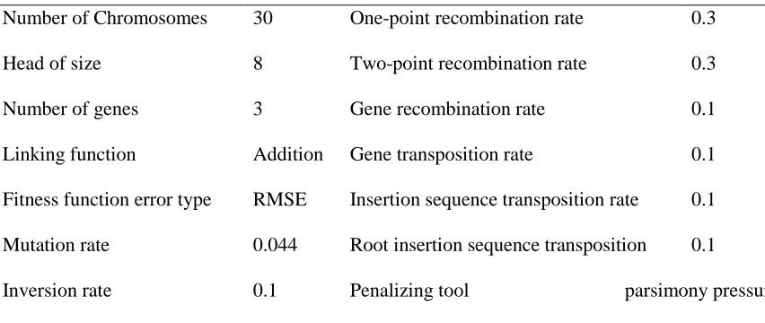
corresponding rates were chosen. Table 3 summarized the commonly used parameters for each
Table 3 Parameters used per run of GEP.
Number of Chromosomes 30 One-point recombination rate 0.3
Head of size 8 Two-point recombination rate 0.3
Number of genes 3 Gene recombination rate 0.1
Linking function Addition Gene transposition rate 0.1
Fitness function error type RMSE Insertion sequence transposition rate 0.1
Mutation rate 0.044 Root insertion sequence transposition 0.1
Inversion rate 0.1 Penalizing tool parsimony pressure
The SVM is developed by Cortes and Vapnik [47] and known as classification and regression
method [33] to solve problems with applying a flexible representation of the class boundaries
and implementing an automatic complexity control to reduce over fitting. In SVM, the
dependency of dependent variable to a set of independent variables is evaluated. In regression
estimation with Support Vector Regression (SVR), which is used to define SVMs in the
literature, a functional dependency 𝑓(𝑥) between a set of sampled input points 𝑋 =
{𝑥1, 𝑥2, 𝑥3, … , 𝑥𝑙} (here, input sampled refer to meteorological variables) taken from 𝑅𝑛 (input
vector of n dimension) and target values 𝑌 = {𝑦1, 𝑦2, 𝑦3, … , 𝑦𝑙} (ETo as target values) with 𝑦𝑖 ∈
𝑅𝑛. More detail on SVM can be found in Vapnik [48].
The LR is statistical method to describe quantitative relationship between a dependent
variable and one or more independent variables [26,49]. In LR, the function is a linear equation
and expressed as:
Where bo-bk are the fitting constants, yi is the dependent variable, and x1-xk are the independent
variables for this system.
The RF method combines a group of decision trees for either classification or regression
purposes. Although each decision tree may not capable of well learning, combination of decision
trees results a strong learner. Each decision tree predicts the outcome individually, and RF votes
among the outcomes for classification or averages the outcomes for regression. Each decision
tree is trained on different subset of samples by a bagging extension of the RF model to reduce
the risk of overfitting. Moreover, different subset of input variables can be used in each tree to
make it more useful in prediction for datasets with higher dimensions [50]. For this study, a
small subset of data was used to find a good combination of parameters for the RF model. As a
result, number of trees in the forest and minimum number of samples required for leaf node were
50 and 35, respectively. The mean square error criteria used as a procedure for estimation.
The calculated daily ETo for was used to feed the GEP, SVM, LR and RF models.
Three treatments including temperature, radiation, and mass transfer-based combinations were
used as input to feed the models and each model of the combinations were assessed for spatial
and temporal approaches. Different statistical analysis was performed to evaluate the accuracy
and performance of the different combinations and approaches for each study stations. The
combinations were as follow:
(i) Tmin, Tmax: temperature based (GEP1, SVM1, LR1, RF1)
(ii) Tmin, Tmax, Rs: radiation based (GEP2, SVM2, LR2, RF2)
2.3 K-fold cross validation
Splitting the data to the sets of data for testing and training is a usual procedure for assessing
the ML techniques. Using 10-30% of the complete data set as a single test set is a common way
for GEP evaluation. Therefore, the K-fold cross validation technique was used to increase the
evaluation performance and set of data for either training or testing purposes. Using K-fold cross
validation, the data set was divided into K subsets, and training process was repeated K times
leaving each time a distinct set of patterns for testing until a complete testing scan for the data set
was fulfilled. Computation cost defines the minimum assemble size of the test set. Here, the
minimum test size was fixed as one year for local modeling and one station for spatial modeling.
Consequently, at local scale, one year was held out each time for testing while the models were
trained using the remaining 16 years; hence, a total of 612 models (17 years× 6 stations× 3 input
combinations× 2 models) were established for the local k-fold testing. At the spatial scale, one
station was considered as test block each time and the models were trained using the patterns
from the remaining stations; hence, a total number of 36 models (6 stations× 3 input
combinations× 2 models) were constructed. The temporal and spatial approaches were noted
with T and S in the figures.
2.4 Evaluation criteria
To investigate the performance of models for each combinations and approaches, four
statistical indicators were used, namely, the root mean square error (RMSE), the mean absolute
error (MAE), correlation coefficient (r2), and scatter index (SI), defined as follows:
𝑅𝑀𝑆𝐸 = √1
𝑛∑ (𝐸𝑇𝑒− 𝐸𝑇𝑜) 2 𝑛
𝑀𝐴𝐸 =∑𝑛𝑖=1|𝐸𝑇𝑒−𝐸𝑇𝑜|
𝑛 (4)
𝑟2 = ( ∑𝑛𝑖=1(𝐸𝑇𝑜−𝐸𝑇̅̅̅̅̅)(𝐸𝑇𝑜 𝑒−𝐸𝑇̅̅̅̅̅)𝑒
√∑𝑛𝑖=1(𝐸𝑇𝑜−𝐸𝑇̅̅̅̅̅)𝑜 2∑𝑛𝑖=1(𝐸𝑇𝑒−𝐸𝑇̅̅̅̅̅)𝑒 2
)2 (5)
𝑆𝐼 =𝑅𝑀𝑆𝐸
𝐸𝑜
̅̅̅̅ (6)
where ETe and ETo are simulated and calculated reference evapotranspiration at the i-th time
step, respectively, n is number of time steps, ET̅̅̅̅̅e and ET̅̅̅̅̅o are mean values of simulated and
calculated ETo, respectively.
The RMSE describes the average magnitude of errors and can take on values from 0 to ∞ to
indicate perfect and worst fit, respectively, and the MAE scores the error magnitudes without any
specific weight to larger/smaller errors. Therefore, the lower value of the RMSE and MAE are
desirable. The r2 values around 1 indicates a perfect linear relationship between estimated and
calculated values, which the closer value to zero demonstrate the poor relationship between
simulation and calculation. Finally, SI is a dimensionless index of RMSE that gives a good
insight to compare the performance of different models.
3 Results and Discussions
The local (or temporal) and spatial analysis of four models for six study stations are shown in
table 3. According to the three combinations’ performance, radiation-based method illustrated
the highest accuracy for either local or spatial approaches compared to the other combinations.
The mass-transfer based combination was the next accurate combination. Results showed that
the local trained models surpassed the spatially trained models because of using the same
results compared to the local model in some cases, especially for radiation-based combinations.
Differences of temperature among the stations was dramatically affected the performance of both
temperature-based and mass transfer-based models. In all cases, minimum differences between
the performance accuracy of the local and spatial models were belonged to the LR model. This
can be inferred to the mathematical structure of this technique, where only linear relationships
can be supposed between the input and target parameters with lower degree of flexibility
compared to heuristic data driven models.
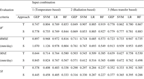
Table 3 Global average performance indicators of the gene expression programming (GEP), support vector machine (SVM), multiple linear regression (LR), and random forest (RF) for three
input combinations of local (T) and spatial (S) approaches.
Among four models with three input combinations, the models relying on radiation,
mass-transfer, and temperature-based combinations showed the lowest RMSE and MAE, respectively
(table 3). Comparing the GEP, SVM, LR and RF models, the RF model illustrated the lowest rate Evaluation
criteria
Input combination
1 (Temperature-based) 2 (Radiation-based) 3 (Mass-transfer based)
Approach GEP SVM LR RF GEP SVM LR RF GEP SVM LR RF
of RMSE and MAE with the best performance for radiation-based approaches. However, the RF
model improved 4.37, 5.76 and 1.49 percent from local to spatial approaches for temperature,
radiation, and mass-transfer based combinations, respectively, which was in contrast with the
improvement’s direction of the other models. Considering the models on the basis of radiation
combination, the spatial RF model exhibited the highest linear relationship (r2=0.927) between
calculated and estimated ETo in comparison with the other models. The local RF method was the
next accurate approach to estimate ETo based on radiation-based data. This observation
illustrated the ability of the RF algorithms to estimate ETo using data from local stations for
training. Furthermore, the LR model had significant improvement for RMSE and MAE from
spatial to local approaches for all three types of input combinations. For LR model, the r2 value
was not changed for radiation-based and temperature-based combination from spatial to local
approaches and the change was 0.13 percent for mass-transfer based model. Therefore, the LR
model illustrated almost similar result for both spatial and local approaches among all models.
The GEP and SVM models illustrated the great improvement rate for all three input
combinations from spatial to local condition with the highest improvement of 21 percent for
mass-transfer based combination. Specifically, the GEP model showed an improvement from
spatial to temporal approach, however, the percentage of improvement was 2.3, 3.9, and 0.13 for
radiation, temperature and mass-transfer based combinations, respectively. In term of obtained
improvement for RMSE and MAE from spatial to local approaches, both of the GEP and SVM
models gained the similar results. The correlation coefficient of the SVM model decreased from
spatial to local approaches for about 6.3, 6.5, and 10.9 percent for radiation, temperature and
mass-transfer based combinations, respectively. By using local radiation data for training the
percent from spatial to local approach, respectively. This improvement was about 6.6 and 8.7
percent for mass-transfer based and 15 and 10.9 percent for temperature-based combinations,
respectively.
Statistical analysis revealed the similar performance of the local GEP and SVM models. For
RMSE and MAE statistical variables, GEP and SVM models showed the greater improvement in
performance for mass-transfer and temperature-based combinations, respectively. By considering
correlation coefficient values, it can be concluded that the improvement in accuracy of either
GEP or SVM approaches were not significant and all illustrated the ability to estimate with an
acceptable accuracy. Therefore, if temperature data were not available at the station, but they do
for other stations, the GEP and SVM approaches can be useful to estimate ETo. However, due to
the higher mapping ability of the GEP models, using either local or spatial GEP are preferable.
The models relying on the mass-transfer combination had slightly higher accuracy than the
temperature-based approach, but lower accuracy compared to the radiation-based combination.
All of the local and spatial GEP and SVM methods illustrated lower improvement compared to
than that for the temperature-based approach. This showed that wind speed can have a significant
effect on accurate estimation of spatial and local ETo. Due to the flat topography of the study
area and facing with lots of high-speed winds during the growing season and almost other
seasons, including the wind as a parameter to build the model architecture and estimating the ETo
can increase the accuracy of the approach.
Overall, the RF and the LR models illustrated the best performance among the four models,
and comparing the GEP and SVM models, the GEP model showed better performance than SVM
A breakdown of the models’ performance accuracy at each station are shown in Figures 1-3
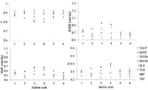
for all of the three input combinations, respectively. In case of the temperature-based
combination (Figure 1), the local GEP and SVM models (shown as: TGEP and TSVM) gave
more accurate results than the spatial (shown as: SGEP and SSVM) models. For the LR and RF
models, the difference of accuracy between local (TLR and TRF) and spatial approaches (SLR
and SRF) were not significant and both showed better performance than GEP and SVM models
since they relied on the patterns of the same location used for training and testing the models.
According to table 2, station 6 (Fargo) had highest and station 2 (Galesburg) had lowest range of
recorded temperature among the study stations. This range may be caused to have the lowest
performance for station 2; however, it was difficult to evaluate the model performance in the
climate context of each station due to the few numbers of study stations. The RF model showed
the best performance with higher accuracy for all stations either temporally or spatially, and the
Figure 1. Statistical indices of the temperature-based combination for four applied models (GEP, VM, LR and RF) with local (T) and spatial (S) approaches
The RF and LR methods showed the lowest range of SI compared to the spatial and local
GEP and SVM methods. For temperature-based combination, the spatial and local LR
approaches had minimum SI ranges of 0.018 and 0.020, respectively, and the spatial SVM and
GEP methods illustrated the highest SI ranges of 0.113 and 0.119, respectively. The spatial RF
approaches with an average of 0.333, and spatial SVM with an average of 0.457 showed the
lowest and highest SI rate, respectively. Therefore, spatial RF approaches may be the practical
way to estimate the missing meteorological data of the study stations.
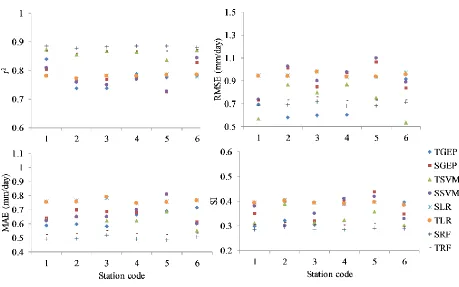
Figure 2 shows evaluation result of the radiation-based combination for the four models with
spatial and local approaches. The amount of received radiation for all study stations were similar.
the best performance among the three input combinations. In addition, the radiation-based
combination had the lowest rate of RMSE, MAE, and SI, and the highest rate of r2 for each of the
study stations. Among the spatial and local scenarios, local approach had the better performance
than the spatial approach. For the radiation-based combination, the spatial RF and local RF
models had an accurate estimation of ETo, respectively. For station 3 and 4 (Leonard and Sabin)
either spatial or local approaches of GEP and SVM models gained lower performance than the
other stations. This can be due to the slightly higher magnitude and variations of solar radiation
(table 2) among the other stations during the study period.
Figure 2. Statistical indices of radiation-based combination for four applied models (GEP, SVM, LR and RF) with local (T) and spatial (S) approaches
Among the study stations comparison, the SI range of the spatial RF was 0.018, which
temperature-based combination, the LR method performed well in radiation-based combination
too, with SI indicator range of 0.021 and 0.024 for temporal and spatial LR approaches,
respectively. The worst performance was observed for spatial GEP and SVM approaches, with
SI indicator of 0.128 and 0.140, respectively. According to the GEP and SVM models, the local
GEP performed well compared to other approaches of the SVM and GEP models. The statistical
indicators were in agreement with the spatial RF performance in which showed the lowest rate of
RMSE and MAE and highest value of r2. However, comparing the MAE might not be a valid
indicator due to taking into account the local order of magnitude of the target variable. The
ranking of the SI indicators showed that spatial RF and LR could overcome the lack of
meteorological data for the station. On the other hand, the averages of the SI values for all 6
study stations showed that the spatial RF and temporal RF had the lowest and the spatial GEP
and spatial SVM had the highest rate of SI indicators. Therefore, either spatial or temporal RF
method could be useful to estimate the missing values for any of the stations.
Figure 3 shows the statistical indices of the mass-transfer based combination. Similar to the
previous combinations, the spatial and local RF gave the accurate estimation than other methods.
On the other hand, the local SVM approach showed better estimation than spatial SVM and GEP
methods for all stations except station 2, which had the lowest range of temperature variation.
The fluctuations of the indices among the stations were higher than radiation-based combination
and lower than that for temperature-based combination, which showed the mediocre accuracy
Figure 3. Statistical indices of mass transfer-based combination for four applied models (GEP, SVM, LR and RF) with local (T) and spatial (S) approaches
By having wind speed and temperature data as input variable for the mass transfer-based
combination, spatial RF approach gained the lowest SI and highest r2 values for ETo estimation
compared to the all other methods. The minimum and maximum SI values for mass
transfer-based combination obtained for the spatial RF and spatial SVM approaches, which were 0.011
and 0.120, respectively. According to the performance ranking of the models based on the SI
indicator, spatial LR, local LR, and local RF showed better performance after spatial RF with SI
values of 0.015, 0.018, and 0.018, respectively. The local SVM, local GEP, and spatial GEP had
the SI values of 0.087, 0.10 and 0.119, respectively. The average of SI for all study stations
showed that the temporal and local LR had the highest and spatial and local RF had the lowest SI
values, respectively. Therefore, by having the lowest range of SI and lowest value of SI for
training a specific model for each station. Accordingly, no local dataset could be needed to train
the local models. This could be helpful to estimate the ETo for stations with partial or missing
meteorological data.
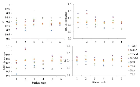
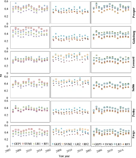
To understand the performance of the applied models on yearly based at each of the study
stations, the models were assessed per test years. Figure 4 illustrates the SI values obtained from
the three input combinations for each study years of the study stations. The SI values of the
models fluctuated considerably for almost all stations during the test years.
As shown in figure 4, the SI values fluctuated considerably within test years for all input
combinations and approaches. Among the study stations, Prosper and Sabin stations showed the
average maximum range for the SI values. The minimum average of the SI value 0.223 was
observed for the RF radiation-based combination for the Fargo station, and the maximum
average of the SI was obtained for the SVM temperature-based combination (SVM1) for the
Galesburg station. The Galesburg station had the lowest temperature range among the study
stations. According to the figure 4, the RF2 (radiation-based combination) model showed the
lowest fluctuation compared to the other approaches with similar trend among the study stations.
For all of the study stations, test years, and input combinations, the RF models gave the best
performance with lowest SI values compared to the other models and combinations. The SVM
and GEP models showed the worst SI averages for the temperature-based combinations. In this
case, the order of the accuracy of the models was similar to that obtained from the station-based
analysis. The radiation-based combination gave the most accurate results and estimation in
Figure 4. Scatter index (SI) values of GEP, SVM, LR, and RF models per test year and study station for three input combinations
Comparing the performance of the models relying on each of the combination methods, it
indicator for different approaches were different depending on the test years. For example, 2011,
2012, and 2013 was the dry, normal, and wet years among the study years, respectively. The
result of SI per test years showed that the 2012 had lower SI than 2011 and 2013 for all of the
three input combinations, and the SI values of the various methods and approaches were close
together. On the other hand, for 2013 test year, some of the approaches illustrated the huge jump
for the obtained SI from 2012 to 2013 due to the weakness of the model performance.
Due to the variability in the meteorological data and the climate pattern, the variability in
performance accuracy at each station was expected. Selection of the training set and testing set
plays an important rule on model performance. Existing of any abnormal year in test year in
comparison with training datasets cause to have an inaccurate estimation (Shiri et al. 2014). By
lowering the number of the input values, the validity of training set for estimation of test years
decrease. Because of the lower input values, the variance rate would be low, and this type of
input only would be valid for periods with very specific trends. This explanation may clarify the
performance of spatial approaches, where relationship encountered might be site specific.
The comparison of the three input combinations showed that the performance of some
approaches was similar for some years while the performance of methods for some years were
far from each other’s. For example, the SVM model showed the most improvement from
temperature to mass-transfer based combination which became like the RF method. However,
depending on the station and test year, this similarity become even closer. All the test years and
stations showed an improvement from temperature to radiation or mass-transfer based
combination except for the Prosper station. On the other hand, the Prosper station showed the
best improvement for SVM model for radiation-based approaches. Considering that all of the
it might be thought that the performance differences could be due to the effect of the second
variable in the estimation of the output. In addition, when the performance of the models is
similar, the impact of secondary variable might be less than the primary variable (temperature).
However, when the gap between the performance or SI indicator increase, it proves the crucial
impact of the secondary variable on the model performance for the specific test year or station.
Similar conclusion could be drawn for the comparison between the input combinations. If each
of the combinations shows the better performance than the other combination method for
specific year and station, the second variable effect should be important and might have
significant influence in the explanation of the output for that test year.
4 Conclusions
The aim of this paper was to evaluate the different ML methods including GEP, SVM, LR
and RF to estimate ETo in the Red River Valley. Global comparison of performance accuracy of
the applied models revealed that the RF model was the best for all combinations among the four
defined models. Furthermore, the RF model illustrated the best performance for spatial and local
conditions for all input combinations. In general, the LR, GEP and SVM models were improved
when a local approach was used, with an exception of the RF model, which was less accurate
with a local approach. The radiation-based combination was the most accurate predictor among
all models tested. As a result, this combination showed the lowest rate of improvement due to
better performance at the first step.
The results showed that due to the flat topography of the study area with high wind speeds
during the growing season, including the wind as a parameter to build the model architecture and
estimate the ETo can increase the accuracy of the prediction. In addition, it might be more
need for local training. The recommended application of spatial RF using radiation combination
allows for a more reliable estimate of ETo to fill the missing values for more precision water
management purposes. Further research should confirm the current results in other geographical
locations and for the various input combination methods.
References
1. Allen, R.G.; Pereira, L.S.; Howell, T.A.; Jensen, M.E. Evapotranspiration information
reporting: I. Factors governing measurement accuracy. Agric. Water Manag. 2011, 98, 899–920.
2. Niaghi, A.R.; Majnooni-Heris, A.; Haghi, D.Z.; Mahtabi, G. Evaluate several potential
evapotranspiration methods for regional use in Tabriz, Iran. J. Appl. Environ. Biol. Sci.
2013, 3, 31–41.
3. Anderson, M.C.; Allen, R.G.; Morse, A.; Kustas, W.P. Use of Landsat thermal imagery in
monitoring evapotranspiration and managing water resources. Remote Sens. Environ.
2012.
4. Kabenge, I.; Irmak, S.; Meyer, G.E.; Gilley, J.E.; Knezevic, S.; Arkebauer, T.J.;
Woodward, D.; Moravek, M. Evapotranspiration and surface energy balance of a common
reed-dominated riparian system in the platte river Basin, Central Nebraska. Trans. ASABE
2013, 56, 135–153.
5. O’Brien, P.L.; Acharya, U.; Alghamdi, R.; Niaghi, A.R.; Sanyal, D.; Wirtz, J.; Daigh,
A.L.M.; DeSutter, T.M. Hydromulch Application to Bare Soil: Soil Temperature
6. Niaghi, A.R.; Jia, X.; Scherer, T.F.; Steele, D.D. Measurement of Non-Irrigated Turfgrass
Evapotranspiration Rate in the Red River Valley. Vadose Zo. J. 2019, 18:180202, doi:10.2136/vzj2018.11.0202.
7. Chávez, J.L.; Howell, T.A.; Copeland, K.S. Evaluating eddy covariance cotton ET
measurements in an advective environment with large weighing lysimeters. Irrig. Sci.
2009.
8. Valayamkunnath, P.; Sridhar, V.; Zhao, W.; Allen, R.G. Intercomparison of surface
energy fluxes, soil moisture, and evapotranspiration from eddy covariance, large-aperture
scintillometer, and modeling across three ecosystems in a semiarid climate. Agric. For.
Meteorol. 2018, 248, 22–47.
9. Niaghi, A R.; Haji Vand, R; Asadi, E; A, Majnooni-Heris. Evaluation of Single and Dual
Crop Coefficient Methods for Estimation of Wheat. Adv. Environ. Biol. 2015, 9, 963–971. 10. Elnmer, A.; Khadr, M.; Kanae, S.; Tawfik, A. Mapping daily and seasonally
evapotranspiration using remote sensing techniques over the Nile delta. Agric. Water
Manag. 2019, 213, 682–692.
11. Nagler, P.L.; Scott, R.L.; Westenburg, C.; Cleverly, J.R.; Glenn, E.P.; Huete, A.R.
Evapotranspiration on western U.S. rivers estimated using the Enhanced Vegetation Index
from MODIS and data from eddy covariance and Bowen ratio flux towers. Remote Sens.
Environ. 2005.
12. Wagle, P.; Bhattarai, N.; Gowda, P.H.; Kakani, V.G. Performance of five surface energy
balance models for estimating daily evapotranspiration in high biomass sorghum. ISPRS J.
13. Partal, T.; Cigizoglu, H.K. Prediction of daily precipitation using wavelet-neural
networks. Hydrol. Sci. J. 2009, 54, 234–246.
14. Torres, A.F.; Walker, W.R.; McKee, M. Forecasting daily potential evapotranspiration
using machine learning and limited climatic data. Agric. Water Manag. 2011, 98, 553– 562.
15. Fan, J.; Yue, W.; Wu, L.; Zhang, F.; Cai, H.; Wang, X.; Lu, X.; Xiang, Y. Evaluation of
SVM, ELM and four tree-based ensemble models for predicting daily reference
evapotranspiration using limited meteorological data in different climates of China. Agric.
For. Meteorol. 2018, 263, 225–241.
16. Shiri, J.; Kişi, Ö.; Landeras, G.; López, J.J.; Nazemi, A.H.; Stuyt, L.C.P.M. Daily
reference evapotranspiration modeling by using genetic programming approach in the
Basque Country (Northern Spain). J. Hydrol. 2012, 414–415, 302–316.
17. Kisi, O.; Guven, A. Evapotranspiration Modeling Using Linear Genetic Programming
Technique. J. Irrig. Drain. Eng. 2010, 136, 715–723.
18. Shiri, J.; Nazemi, A.H.; Sadraddini, A.A.; Landeras, G.; Kisi, O.; Fakheri Fard, A.; Marti,
P. Comparison of heuristic and empirical approaches for estimating reference
evapotranspiration from limited inputs in Iran. Comput. Electron. Agric. 2014, 108, 230– 241.
19. Wen, X.; Si, J.; He, Z.; Wu, J.; Shao, H.; Yu, H. Support-Vector-Machine-Based Models
for Modeling Daily Reference Evapotranspiration With Limited Climatic Data in Extreme
20. Kisi, O. Evapotranspiration modelling from climatic data using a neural computing
technique. Hydrol. Process. 2007, 21, 1925–1934.
21. Odhiambo, L. O.; R. E. Yoder; D. C. Yoder; J. W. Hines Optimization of Fuzzy
Evapotranspiration Model Through Neural Training With Input– Output Examples. Trans.
ASAE 2013, 44, 1625–1633.
22. Trajkovic, S.; Todorovic, B.; Stankovic, M. Closure to “Forecasting of Reference
Evapotranspiration by Artificial Neural Networks” by Slavisa Trajkovic, Branimir
Todorovic, and Miomir Stankovic. J. Irrig. Drain. Eng. 2005, 131, 391–392.
23. Falamarzi, Y.; Palizdan, N.; Huang, Y.F.; Lee, T.S. Estimating evapotranspiration from
temperature and wind speed data using artificial and wavelet neural networks (WNNs).
Agric. Water Manag. 2014, 140, 26–36.
24. Hassan, M.A.; Khalil, A.; Kaseb, S.; Kassem, M.A. Exploring the potential of tree-based
ensemble methods in solar radiation modeling. Appl. Energy 2017, 203, 897–916.
25. Feng, Y.; Cui, N.; Gong, D.; Zhang, Q.; Zhao, L. Evaluation of random forests and
generalized regression neural networks for daily reference evapotranspiration modelling.
Agric. Water Manag. 2017, 193, 163–173.
26. Tabari, H.; Kisi, O.; Ezani, A.; Hosseinzadeh Talaee, P. SVM, ANFIS, regression and
climate based models for reference evapotranspiration modeling using limited climatic
data in a semi-arid highland environment. J. Hydrol. 2012, 444–445, 78–89.
27. Shirsath, P.B.; Singh, A.K. A Comparative Study of Daily Pan Evaporation Estimation
1571–1581.
28. Pour-Ali Baba, A.; Shiri, J.; Kisi, O.; Fard, A.F.; Kim, S.; Amini, R. Estimating daily
reference evapotranspiration using available and estimated climatic data by adaptive
neuro-fuzzy inference system (ANFIS) and artificial neural network (ANN). Hydrol. Res.
2013, 44, 131.
29. Feng, Y.; Peng, Y.; Cui, N.; Gong, D.; Zhang, K. Modeling reference evapotranspiration
using extreme learning machine and generalized regression neural network only with
temperature data. Comput. Electron. Agric. 2017, 136, 71–78.
30. Vogt, M. Support Vector Machines for Identification and Classification Problems in
Control Engineering. - Autom. 2008, 56, 391–391.
31. Singh, R.; Helmers, M.J. Improving crop growth simulation in the hydrologic model drain
mod to simulate corn yields in subsurface drained landscapes. Am. Soc. Agric. Biol. Eng.
Annu. Int. Meet. 2008 2008, 2, 856–873.
32. Wu, W.; Wang, X.; Xie, D.; Liu, H. Soil water content forecasting by support vector
machine in purple hilly region. In IFIP International Federation for Information
Processing; Springer US: Boston, MA, 2008; Vol. 258, pp. 223–230 ISBN
9780387772509.
33. Kisi, O.; Cimen, M. Reply to the Discussion of “Evapotranspiration modelling using
support vector machines” by R. J. Abrahart et al . . Hydrol. Sci. J. 2010, 55, 1451–1452.
34. Shiri, J.; Kişi, Ö. Comparison of genetic programming with neuro-fuzzy systems for
1701.
35. Sanford, W.E.; Selnick, D.L. Estimation of Evapotranspiration Across the Conterminous
United States Using a Regression With Climate and Land-Cover Data. J. Am. Water
Resour. Assoc. 2013, 49, 217–230.
36. Perugu, M.; Singam, A.J.; Kamasani, C.S.R. Multiple Linear Correlation Analysis of
Daily Reference Evapotranspiration. Water Resour. Manag. 2013, 27, 1489–1500.
37. Khoshravesh, M.; Sefidkouhi, M.A.G.; Valipour, M. Estimation of reference
evapotranspiration using multivariate fractional polynomial, Bayesian regression, and
robust regression models in three arid environments. Appl. Water Sci. 2015, 7, 1911–1922. 38. Alipour, A.; Yarahmadi, J.; Mahdavi, M. Comparative Study of M5 Model Tree and
Artificial Neural Network in Estimating Reference Evapotranspiration Using MODIS
Products. J. Climatol. 2014, 2014, 1–11.
39. Pérez, J.Á.M.; García-Galiano, S.G.; Martin-Gorriz, B.; Baille, A. Satellite-based method
for estimating the spatial distribution of crop evapotranspiration: Sensitivity to the
priestley-taylor coefficient. Remote Sens. 2017, 9.
40. Shiri, J. Improving the performance of the mass transfer-based reference
evapotranspiration estimation approaches through a coupled wavelet-random forest
methodology. J. Hydrol. 2018, 561, 737–750.
41. NDAWN North Dakota Agricultural Weather Network Available online:
https://ndawn.ndsu.nodak.edu/.
ASCE-EWRI Standardization of Reference Evapotranspiration Task Committe Report. Am. Soc.
Civ. Eng. 2005.
43. Angeline, P.J. Genetic programming: On the programming of computers by means of
natural selection,. Biosystems 2003, 33, 69–73.
44. Ferreira, C. Gene Expression Programming: a New Adaptive Algorithm for Solving
Problems. 2001.
45. Sharifi, S.S.; Rezaverdinejad, V.; Nourani, V. Estimation of daily global solar radiation
using wavelet regression, ANN, GEP and empirical models: A comparative study of
selected temperature-based approaches. J. Atmos. Solar-Terrestrial Phys. 2016, 149, 131– 145.
46. Shiri, J.; Sadraddini, A.A.; Nazemi, A.H.; Kisi, O.; Landeras, G.; Fakheri Fard, A.; Marti,
P. Generalizability of Gene Expression Programming-based approaches for estimating
daily reference evapotranspiration in coastal stations of Iran. J. Hydrol. 2014, 508, 1–11.
47. Cortes, C.; Vapnik, V. Support-Vector Networks. Mach. Learn. 1995, 20, 273–297. 48. Vapnik, V. The Support Vector Method of Function Estimation. In Nonlinear Modeling;
Springer US: Boston, MA, 2011; pp. 55–85.
49. Azimi, V.; Salmasi, F.; Entekhabi, N.; Tabari, H.; Niaghi, A. Optimization of Deficit
Irrigation Using Non-Linear Programming (Case Study: Mianeh Region, Iran). ijagcs.com
2013, 252–260.
50. Géron, A. Hands-On Machine Learning with Scikit-Learn & TensorFlow; 2017; ISBN