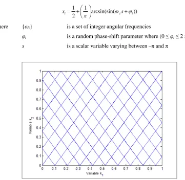
On the importance of input variables and climate variability to the yield of urban water supply systems

(1)

On the Importance of Input Variables and

Climate Variability to the Yield of Urban Water

Supply Systems

by

David Michael King

B. Eng, Civil(Hons), Victoria University

A thesis submitted in fulfilment of the requirements for the degree

of Doctor of Philosophy

School of Engineering and Science

Faculty of Health, Science and Engineering

VICTORIA UNIVERSITY

Australia

(2)

(3)

ABSTRACT

Yield plays a central role in the processes, practices, management and operation of urban water supply systems. In Australia, yield is commonly defined as the maximum average annual volume of water that can be supplied from the water supply system subject to climate variability, operating rules, demand pattern and adopted level of service (or security criteria). For a given water supply system, yield is typically estimated via computational simulation using the entire sequence of available historic climate data. This means that the simulation, and hence the estimation of yield, is subject to a range of extreme climate events consisting of various dry and wet spells with a multitude of severities and durations, present in the historic data. System management policies and rules are optimised to a single climate scenario that may not match the planning length of the studies conducted by the water authority, nor allowing for the effects of future climate variability.

This study is on the importance of input variables and climate variability to the estimation of yield of an urban water supply system. Primarily, the effects of planning period and the climate variability on the yield and on the importance of input variables are assessed.

A preliminary case study on a simple, hypothetical urban water supply system was conducted primarily to assess the applicability and limitations of three sensitivity analysis (SA) techniques, namely the Morris Method, the Fourier Amplitude Sensitivity Test and Sobol’s method of SA. These techniques produced mostly reliable results which revealed some limitations of the SA framework adopted. The findings and conclusions of the preliminary study bore important improvements before use on the complex case study of the Barwon Water supply system.

Employing 20 climate scenarios over four simulation lengths, the input variables used in the estimation of yield for the Barwon urban water supply system were subjected to SA using the above-mentioned techniques. Significant findings of the study showed that the estimation of yield is more volatile to changes in the input variables and climate variability for shorter planning periods. This was indicated by the average and the range of the yield estimate decreasing as the planning length increased.

(4)

(5)

DECLARATION

I, David Michael King, declare that the PhD thesis entitled ‘On the importance of input variables and climate variability to the yield of urban water supply systems’ is no more than 100,000 words in length including quotes and exclusive of tables, figures, appendices, bibliography, references and footnotes.

This thesis contains no material that has been submitted previously, in whole or in part, for the award of any other academic degree or diploma. Except where otherwise indicated, this thesis is my own work.

(6)

(7)

ACKNOWLEDGEMENTS

I would like to thank my supervisor, Professor Chris Perera, for his continued encouragement, support and generosity throughout the progression of this work. He has been a great source of confidence and guidance for me, always providing pertinent and timely advice, and exhausting comments on my work, whilst still respecting my voice. I am truly appreciative of the valuable time and effort that Chris has given me throughout this thesis and I am blessed and honoured to have had worked with such a great supervisor. Additional support in the early stages of this work from Emeritus Professor Michael Hasofer is also greatly appreciated.

I would also like to express my appreciation to Victoria University, for the continuing opportunity to study. I would also like to thank the staff of the (former) School of Architectural, Civil and Mechanical Engineering at VU who supported and helped me throughout my time at VU in both my research and teaching positions. In particular, I would like to express my gratitude to Mr. Greg Evans, who was extremely helpful and supportive, by giving advice and encouragement in an enthusiastic approach to teaching.

The inspiration to undertake this study was in the admiration of Adrian Scholes. Although I knew you briefly, your spirit, energy, modesty and passion for life continue to motivate and inspire me. It was an honour and a privilege knowing you. Thankyou.

(8)

(9)

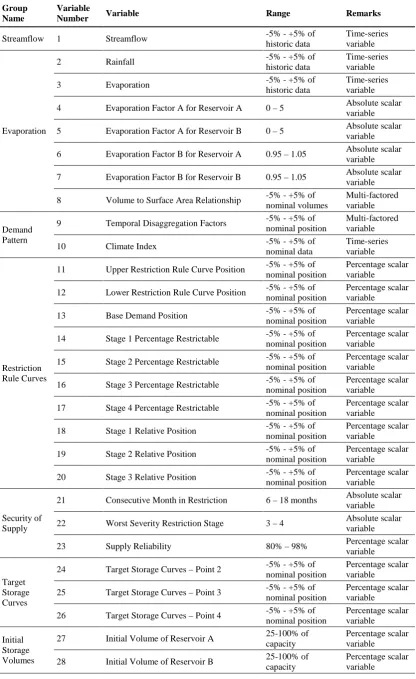
4.1 Introduction ... 4-1 4.2 System Description ... 4-2 4.2.1 Model Input Variables Used in this Study ... 4-3 4.2.1.1 Streamflow Data ... 4-3 4.2.1.2 Evaporation Data ... 4-6 4.2.1.3 Demand... 4-7 4.2.1.4 Temporal Disaggregation Factors ... 4-7 4.2.1.5 Climate Index Data ... 4-8 4.2.1.6 Restriction Rule Curves ... 4-8 4.2.1.7 Target Storage Curves ... 4-10 4.2.1.8 Security of Supply ... 4-11 4.2.1.9 Initial Storage Volumes ... 4-12 4.3 Sensitivity Analysis Framework ... 4-12 4.3.1 Input Variable Handling ... 4-15 4.3.1.1 Streamflow ... 4-15 4.3.1.2 Evaporation ... 4-15 4.3.1.3 Demand Pattern ... 4-17 4.3.1.4 Restriction Rule Curves ... 4-19 4.3.1.5 Security of Supply ... 4-20 4.3.1.6 Target Storage Curves ... 4-21 4.3.1.7 Initial Volume of Reservoirs ... 4-22 4.3.2 Design of Sensitivity Analysis Experiments ... 4-24 4.4 Sensitivity Analysis: The Morris Method... 4-25 4.5 Sensitivity Analysis: Variance Based Methods ... 4-30 4.6 Issues, Limitations and Recommendations ... 4-44 4.7 Summary ... 4-46

CHAPTER 5 SENSITIVITY ANALYSIS USING THE BARWON URBAN

WATER SUPPLY SYSTEM

(12)

5.2.1 Input Variables Used in this Study ... 5-6 5.2.1.1 Climate Dependant Variables ... 5-6 5.2.1.2 Security of Supply ... 5-7 5.2.1.3 Restriction Rule Curves ... 5-8 5.2.1.4 Target Storage Curves ... 5-11 5.3 Sensitivity Analysis Framework ... 5-12 5.3.1 Scenario Selection and Input Variable Handling ... 5-15 5.3.1.1 Scenario Selection ... 5-15 5.3.1.2 Security of Supply ... 5-20 5.3.1.3 Restriction Rule Curves ... 5-24 5.3.1.4 Target Storage Curves ... 5-27 5.3.2 Design of Sensitivity Analysis Experiments ... 5-27 5.4 Sensitivity Analysis Results ... 5-29 5.4.1 Morris Method Results ... 5-29 5.4.1.1 Individual Input Variable Experiments... 5-31 5.4.1.2 Grouping 1 Experiments ... 5-38 5.4.1.3 Grouping 2 Experiments ... 5-43 5.4.1.4 Summary of Morris Experiments ... 5-49 5.4.2 Variance Based Method Results ... 5-50 5.4.2.1 Individual Experiments ... 5-52 5.4.2.2 Grouping 1 Experiments ... 5-64 5.4.2.3 Grouping 2 Experiments ... 5-68 5.5 Issues, Limitations and Recommendations ... 5-74 5.6 Summary ... 5-75

CHAPTER 6 SUMMARY, CONCLUSIONS AND RECOMMENDATIONS

6.1 Summary ... 6-1 6.2 Findings and Conclusions of the Study ... 6-3 6.2.1 Sensitivity Analysis in Water Supply System Modelling ... 6-3 6.2.1.1 Sensitivity Analysis Techniques ... 6-3 6.2.1.2 Variable Handling ... 6-5 6.2.1.3 Additional Sensitivity Analysis Measures ... 6-5 6.2.2 Sensitivity of Yield Estimate to Input Variables ... 6-6 6.2.3 Sensitivity of the Yield Estimate to Planning Length and Climate

(13)

6.3 Limitations of the Study and Recommendations for Further Research ... 6-10

REFERENCES ... 7-1

APPENDIX A Morris Method Algorithm ... A-1 – A-5 APPENDIX B Results of Individual Morris Method Experiments of the

Preliminary Case Study ... B-1 – B-17 APPENDIX C Time-Series Perturbation and Correlation Issues ... C-1 – C-4 APPENDIX D SA Results of eFAST Individual Experiments for the Barwon

Water Supply System Case Study ... D-1 – D-5 APPENDIX E Sobol’ Second-Order Sensitivity Indices of Individual Experiments

(14)

LIST OF FIGURES

Figure 1-1. Average Annual Inflow to the Barwon Urban Water Supply System. ... 1-7

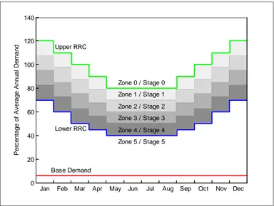
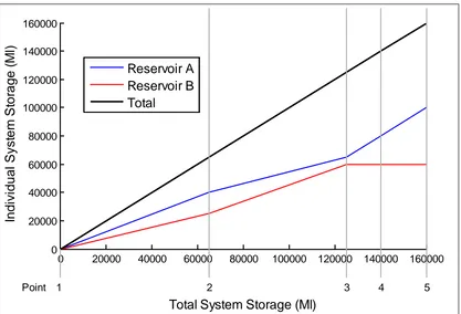
Figure 2-1. Example of a 5-Stage Urban Restriction Rule Curves. ... 2-10 Figure 2-2. Target Storage Curves for a Typical Two-Reservoir System. ... 2-10

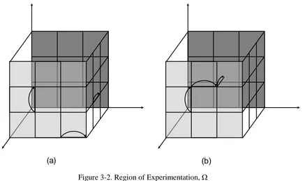
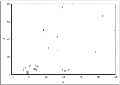
Figure 3-1. Generalised Model Abstraction from Physical System ... 3-3 Figure 3-2. Region of Experimentation, Ω ... 3-28 Figure 3-3. Example of μ – σ Plane used to Present Results of a Morris Method

Experiment ... 3-30 Figure 3-4. Transformation of Two Input Variables using Equation (3.23) ... 3-36

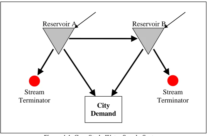
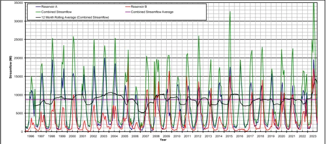
Figure 4-1. Case Study Water Supply System. ... 4-2 Figure 4-2. Monthly Streamflow Data for Reservoir A, Reservoir B and Combined

Streamflow. ... 4-4 Figure 4-3. Nominal Temporal Disaggregation Factors used in this Study. ... 4-7 Figure 4-4. Set of 5-Stage Urban Restriction Rule Curves. ... 4-9 Figure 4-5. Target Storage Curves for the Hypothetical Case Study System. ... 4-11 Figure 4-6. Example of Perturbation Algorithm on Temporal Disaggregation

Factors. ... 4-19 Figure 4-7. Yield Estimate Over 0-100% Initial Storage Volumes. ... 4-23 Figure 4-8. Combined Results of the Morris Method Experiments. ... 4-29 Figure 4-9. First-Order Indices (Si) for Experiments 13, 14, 15 and 16 Indicating

Parity of Results Across all Experiments. ... 4-39

Figure 5-1. Region of Service of the Barwon Water. ... 5-4 Figure 5-2. Headworks of the Barwon Water Region of Service ... 5-5 Figure 5-3. Nominal Restriction Rule Curves for Barwon Urban Water Supply

System. Values given in Table 5-2. ... 5-9 Figure 5-4. Five-Point Target Rule Curves for the Barwon Urban Water Supply

System. ... 5-11 Figure 5-5. Hierarchy of the Sources of Variability of the Estimation of Yield of

(15)

Figure 5-7. Nominal Restriction Rule Curves Showing Percentage of Total System

Capacity. ... 5-21 Figure 5-8. Samples of the Security of Supply Range Tests for 20 Year Planning

Period ... 5-22 Figure 5-9. Samples of the Security of Supply Range Tests for 40 Year Planning

Period ... 5-23 Figure 5-10. Upper and Lower Interpolation Limit Bounds for Perturbation of

Curvature. ... 5-26 Figure 5-11. Grouping Experiment 1. Showing the Evolution of the Morris Indices

for the Restriction Rule Curves Group over 20 Year Planning Period... 5-31 Figure 5-12. µ* Results of the Individual Input Variable Morris Method

Experiment – 20 Year Planning Period. ... 5-33 Figure 5-13. µ* results of the Grouping 1 Morris Method Experiment – 20 Year

Planning Period. ... 5-39 Figure 5-14. µ* results of the Grouping 1 Morris Method Experiment – 40 Year

Planning Period. ... 5-42 Figure 5-17. µ* Results of the Grouping 2 Morris Method Experiment - 20 Year

Planning Period. ... 5-48 Figure 5-21. eFAST Individual Experiment. Reliability of Supply Threshold. Si and

STi Results for all Scenarios. ... 5-55

Figure 5-22. eFAST Individual Experiment. Minimum Storage Level Threshold. Si

and STi Results for all Scenarios. ... 5-55

Figure 5-23. RRCs Si and STi Results for all Scenarios in the eFAST Grouping 1

Experiments. ... 5-66 Figure 5-24. Target Curves Si and STi Results for all Scenarios in the eFAST

(16)

Figure 5-25. Security Criteria Si and STi Results for all Scenarios in the eFAST

Grouping 1 Experiments. ... 5-66

Figure A-1. The Region of Experimentation, Ω. ... A-1

Figure D-1. eFAST Individual Experiment. Relative Position Intermediate Curve 1.

Si and STi Results for all Scenarios. ... D-1

Figure D-4. eFAST Individual Experiment. Percentage Restricatable Zone 1. Si and

STi Results for all Scenarios. ... D-2

Figure D-7. eFAST Individual Experiment. Upper RRC Curvature. Si and STi

Results for all Scenarios. ... D-3 Figure D-8. eFAST Individual Experiment. Upper RRC Position. Si and STi Results

for all Scenarios. ... D-3 Figure D-9. eFAST Individual Experiment. Lower RRC Curvature. Si and STi

Results for all Scenarios. ... D-4 Figure D-10. eFAST Individual Experiment. Lower RRC Position. Si and STi

Results for all Scenarios. ... D-4 Figure D-11. eFAST Individual Experiment. Base Demand Curve Position. Si and

Figure D-12. eFAST Individual Experiment. Target Storage Curves. Si and STi

Results for all Scenarios. ... D-5 Figure D-13. eFAST Individual Experiment. Minimum Storage Level Threshold. Si

and STi Results for all Scenarios. ... D-5

Figure D-14. eFAST Individual Experiment. Reliability of Supply Threshold. Si

(17)

LIST OF TABLES

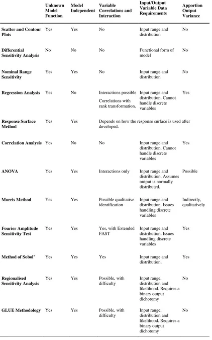
Table 3-1: Uncertainty Typologies from the Literature. ... 3-4 Table 3-2. Alternative Terminology for the Two Distinct Types of Uncertainty. ... 3-6 Table 3-3. Comparison of the Considered SA Techniques Against Ideal Selection

Criteria. ... 3-26

Table 4-1. Statistical Properties of Streamflow into Reservoir A. ... 4-5 Table 4-2. Statistical Properties of Streamflow into Reservoir B. ... 4-5 Table 4-3. Volume to Surface Area Relationship of Reservoir A. ... 4-6 Table 4-4. Volume to Surface Area Relationship of Reservoir B. ... 4-6 Table 4-5. Restriction Rule Curve Values. ... 4-9 Table 4-6. Percentage Restrictable and Relative Position of the Intermediate

Curves. ... 4-10 Table 4-7. Target Storage Curve Values for Simple Case Study. ... 4-10 Table 4-8. Description of Input Variables Used in this Study. ... 4-16 Table 4-9. Reservoir B Sampling Limits for Nominal Total Storage Volumes. ... 4-21 Table 4-10. Algorithm Settings for the Morris Method Sensitivity Analysis

Experiment. ... 4-26 Table 4-11. Combined Results of the Morris Method Experiments. ... 4-28 Table 4-12. Settings of the Preliminary FAST Experiments. ... 4-31 Table 4-13. First-Order Indices (Si) for FAST Experiments 1 and 2 ... 4-33

Table 4-14. First-Order Indices (Si) and Total-Order (STi) for eFAST Experiments 3

and 4 ... 4-34 Table 4-15. First-Order Indices (Si) and Total-Order (STi) for eFAST Experiments 5

and 6 ... 4-35 Table 4-16. First-Order Indices (Si) and Total-Order (STi) for Grouped eFAST

Experiments 7 and 8 ... 4-36 Table 4-17. First-Order Indices (Si) and Total-Order (STi) for Grouped eFAST

Experiments 9 and 10 ... 4-37 Table 4-18. Top 10 Important Variables used in Detailed SA Experiments. ... 4-37 Table 4-19. Settings for the 10 Variable SA Experiments. ... 4-38 Table 4-20. First-Order Indices (Si) for FAST Experiments 11 and 12. ... 4-39

Table 4-21. First-Order Indices (Si) and Total-Order (STi) for eFAST Experiment

(18)

Table 4-23. Pair-Wise Interaction Indices (S_ij) for Sobol’ Experiment 18 ... 4-42 Table 4-24. Closed Pair-Wise Interaction Indices ( c

ij

S ) for Sobol’ Experiment 18 ... 4-43

Table 5-1. Major Storages of the Barwon Urban Water Supply System. ... 5-6 Table 5-2. Nominal Values of the Upper and Lower Rule Curves, Base Demand

and the Intermediate Curves 1, 2 and 3. Relative Positions of the Intermediate

Curves given in Table 5-3. ... 5-10 Table 5-3. Percentage Restrictable and Relative Position of the Intermediate

Curves. ... 5-10 Table 5-4. Nominal Values of the 5-point Target Storage Curves of the Barwon

Water Supply System. ... 5-12 Table 5-5. Description of Input Variables Used in this Study ... 5-16 Table 5-6. 20 Year Planning Length Scenario Selection Data. ... 5-18 Table 5-7. 40 Year Planning Length Scenario Selection Data. ... 5-19 Table 5-8. 60 Year Planning Length Scenario Selection Data. ... 5-19 Table 5-9. Results of the Individual Input Variable Morris Method Experiment – 20

Year Planning Period. ... 5-34 Table 5-10. Results of the Individual Input Variable Morris Method Experiment –

40 Year Planning Period. ... 5-35 Table 5-11. Results of the Individual Input Variable Morris Method Experiment –

60 Year Planning Period. ... 5-36 Table 5-12. Results of the Individual Input Variable Morris Method Experiment –

77 Year Planning Period. ... 5-37 Table 5-13. Assignment of Input Variables for the Grouping 1 Experiments. ... 5-39 Table 5-14. Results of the Grouping 1 Morris Method Experiment – 20 Year

Planning Period. ... 5-39 Table 5-15. Results of the Grouping 1 Morris Method Experiment – 40 Year

Planning Period. ... 5-42 Table 5-18. Assignment of Input Variables for the Grouping 2 Experiments. ... 5-44 Table 5-19. Results of the Grouping 2 Morris Method Experiment - 20 Year

(19)

Table 5-20. Results of the Grouping 2 Morris Method Experiment – 40 Year

Planning Period. ... 5-48 Table 5-23. Si Results of the Individual eFAST Experiment using 1918 Simulations ... 5-53

Table 5-24. STi Results of the Individual eFAST Experiment using 1918

Simulations ... 5-54 Table 5-25. Correlation Matrix of the First-Order Indices (Si) for the eFAST

Individual Experiment. ... 5-56 Table 5-26. Si Results of the Individual Sobol’ Second-Order Experiment Using

6848 Model Simulations. ... 5-58 Table 5-27. STi Results of the Individual Sobol’ Second-Order Experiment using

6848 Simulations. ... 5-59 Table 5-28. Vi Results of the Individual eFAST Experiment using 1918

Simulations. ... 5-61 Table 5-29. Average Yield Estimates for Each Scenario with Individual eFAST

Experiment. ... 5-62 Table 5-30. Standard Deviation of Yield Estimates for Each Scenario with

Individual eFAST Experiment. ... 5-63 Table 5-31. Si and STi Results of the Grouping 1 eFAST Experiment using 979

Simulations. ... 5-65 Table 5-32. Average Yield Estimates for Each Scenario in the Grouping 1 eFAST

Experiments. ... 5-67 Table 5-33. Standard Deviation of the Yield Estimates for Each Scenario in the

Grouping 1 eFAST Experiments. ... 5-68 Table 5-34. Si and STi Results of the eFAST Grouping 2 Experiments using 1862

Simulations. ... 5-69 Table 5-35. Partial Variance and Total Contribution Variance Results of the eFAST

Grouping 2 Experiment using 1862 Simulations. ... 5-71 Table 5-36. Average Yield Estimates for Each Scenario in the eFAST Grouping 2

Experiments. ... 5-72 Table 5-37. Standard Deviation of Yield Estimates for Each Scenario in the eFAST

(20)

Table 6-1. Average Yield Estimate for the Barwon Urban Water Supply System. ... 6-8

Table B-1. Algorithm Settings for the Morris Method Sensitivity Analysis

Experiment. ... B-1 Table B-2. Results of the Morris Method Experiment 1. ... B-2 Table B-3. Results of the Morris Method Experiment 2. ... B-3 Table B-4. Results of the Morris Method Experiment 3. ... B-4 Table B-5. Results of the Morris Method Experiment 4. ... B-5 Table B-6. Results of the Morris Method Experiment 5. ... B-6 Table B-7. Results of the Morris Method Experiment 6. ... B-7 Table B-8. Results of the Morris Method Experiment 7. ... B-8 Table B-9. Results of the Morris Method Experiment 8. ... B-9 Table B-10. Results of the Morris Method Experiment 9. ... B-10 Table B-11. Results of the Morris Method Experiment 10. ... B-11 Table B-12. Results of the Morris Method Experiment 11. ... B-12 Table B-13. Results of the Morris Method Experiment 12. ... B-13 Table B-14. Results of the Morris Method Experiment 13. ... B-14 Table B-15. Results of the Morris Method Experiment 14. ... B-15 Table B-16. Results of the Morris Method Experiment 15. ... B-16 Table B-17. Results of the Morris Method Experiment 16. ... B-17

Table C-1. Analysis of Uniform, Varying and Random Perturbation Methods for a

5% Change... C-2 Table C-2. Top 10 Important Variables used in Detailed SA Experiments. ... C-3 Table C-3. First-Order Indices (Si) for eFAST Perturbation Strategies Experiment. ... C-3

Table C-4. Total-Order Indices (STi) for eFAST Perturbation Strategies Experiment. ... C-4

Table E-1. ‘Closed’ Second-Order Importance Measures (

S

_ijc) of the Sobol'

Experiment for the Barwon Urban Water Supply System Case Study – 20

year Scenario 1. ... E-2

S

(21)

S

ijc) of the Sobol'

S

year Scenario 2b. ... E-7

S

year Scenario 2c. ... E-8 Table E-8. Second-Order Importance Measures (Sij) of the Sobol' Experiment for

the Barwon Urban Water Supply System Case Study – 20 year Scenario 1. ... E-9 Table E-9. Second-Order Importance Measures (Sij) of the Sobol' Experiment for

the Barwon Urban Water Supply System Case Study – 20 year Scenario 2b. ... E-14 Table E-14. Second-Order Importance Measures (Sij) of the Sobol' Experiment for

(22)

(23)

Chapter 1 Introduction

1.1 Background

Potable water and its supply systems are viewed as increasingly valuable commodities throughout Australia and the rest of the world. Changing climate and the increasing growth in population has put many water supply systems under immense pressure, often being required to supply a demand which is close to or exceeding its sustainable demand limit, or yield. Such pressures have been exerted on most Australian water supply systems, resulting in record restriction periods and in some cases the introduction of permanent water saving measures (DSE, 2004). Demand shortfalls can be alleviated by decreasing the demand via water saving measures and schemes, and education; and/or increasing the yield of the system by optimising system management and/or augmentation with additional water sources. All of these methods, and many operational processes undertaken by water authorities, rely heavily on the yield of the water supply system.

Yield can be thought of as the maximum volume of water that can be sustainably supplied from the system over a given period. It is subject to inflows, outflows and management rules and policies, and therefore it is a direct indicator of the performance of the system and its management. Not only does it define the maximum target demand, it is also an essential part in water supply system management and policy development and enforcement. It is used in augmentation studies, guides water sharing, and assists in decision-making polices. Optimising the management of an existing water supply system is a continual process that is largely the responsibility of water authorities and their processes and practices. The management and operational improvements of a system ultimately aim at maximising the performance of the system, namely the yield of the system. However, the estimation of the yield of a system contains various sources of uncertainty, such as the natural variability inherently implicated in being affected by climatic events, and the lack of knowledge of the optimum set of management policies and rules, which themselves are subject to climatic events.

(24)

stakeholder requirements. These operations, policies and rules are input variables in the estimation of yield of the system. This method is based on only one climate scenario and provides no flexibility to assess the impact of different climate realisations or to observe the effects of different planning lengths. Furthermore, it implies that there is a fixed set of optimised system policies and rules for any and all future scenarios.

The use of computational modelling is a critical element in the processes, practices, management and operation of urban water supply systems. However, uncertainty exists throughout all aspects of managing and modelling urban water supply systems, from the collection and handling of data, the interpretation of the physical system into a computational simulation, accuracy of future predictions, value of input variables, operation of the model, etc. This uncertainty propagates through the model to the model output: the yield. Following, this uncertainty in the estimation of yield will be instilled onto any management policies derived from the yield estimate. Although the exact realisation of yield is impossible to obtain (due to the variability that occurs from climate events and lack of knowledge of the optimal position of the system polices, rules and thresholds), certainty in its estimation can be improved by identifying highly influential input variables, and investigating and refining their knowledge. This will improve the confidence in the yield estimate and any management procedures and processes that consider it, leading to optimised system policy development and enforcement, augmentation studies, water sharing strategies and other decision-making practices, as well as an optimal target demand.

The yield of a water supply system is dependant on numerous variables including data (e.g. streamflow and demand), empirical inputs (e.g. operating rules), and model parameters. As these inputs are determined through either measurement, optimisation or modeller experience, they inherently contain unquantified errors which are conveyed through the model structure to the output. Minimising these errors will increase the confidence in the output, or yield. However, input variables may have different significance in terms of their influence on the output. Therefore, it is desirable to identify, investigate and improve the input variables that have considerable effects on the output. The identification of important variables is a primary goal of Sensitivity Analysis (SA).

(25)

study, the SA will assess how perturbations to input variables effect the estimation of yield. The application of SA to a given problem is potentially powerful in identifying, assessing and measuring the importance of the input variables on the model and its output. The success depends on the applicability of the SA framework adopted, specifically the aptness of the selected technique(s), design of SA experiments, accuracy required and determined, and the examination of the results.

1.2 Aims of the Study

The aim of this study was to identify the importance of the variables used in the estimation of yield of an urban water supply system. Understanding the importance of the variables used in the estimation of yield provides an indication as to where water authorities should prioritise research and focus their resources to improve the understanding of the input variables. Greater understanding of the input variables used in the estimation of the yield will improve the confidence of its estimation, leading to optimised management procedures and policies, as well as more reliable target demand.

The first case study used in this research employed a simple, hypothetical urban water supply system as a proof-of-concept study to assess the adopted SA techniques and framework, and to provide preliminary results. A number of limitations, findings and conclusions became apparent whilst attempting to achieve the above aim using this hypothetical model. The principal deficiencies were in the adopted definition of yield and the associated handling of time series variables, such as streamflow and rainfall.

(26)

To achieve the modified aim, a series of SA experiments were used to identify and quantify the sensitivity of the model, and its output(s), to changes in the model inputs. The sensitivity of the model and yield to changes in the model inputs will be observed under different climate realisations, giving an indication of the need for a dynamic set of policies and rules that accommodate possible future climate realisations. Furthermore, by assessing the sensitivity of the model to changes in the input variables over different planning lengths, the necessity of using the same or similar simulation period (in the simulation of the water supply model) as the planning length of the system studies will become apparent.

1.3 Research Methodology

To achieve the above aims, several denotable steps were used:

1. Review of SA theory and SA techniques

2. Design of SA framework for the preliminary case study

3. Conduct SA on preliminary study and review findings

4. Design of SA framework for the Barwon urban water supply system case study

5. Conduct SA on the Barwon system and review findings

Task 1 – Review of SA theory and SA techniques

A review of uncertainty and sensitivity theory highlighted the difference between the two and introduced the significance and purpose of SA. A number of the more modern and commonly used SA techniques were then examined. Each technique was assessed against several ideal characteristics for application to the urban water supply system models, considering the input/output types and structure, the model type and availability, the accuracy and computational requirements. From this review three SA techniques were selected to assess the sensitivity of the estimation of yield to input variable perturbations, namely the Morris method, the Fourier Amplitude Sensitivity Test (FAST) and Sobol’s method of sensitivity analysis. The extended Fourier Amplitude Sensitivity Test (eFAST) was also selected as a natural extension to the original FAST.

Task 2 – Design of SA framework for the preliminary case study

(27)

to an urban water supply system model, and to uncover limitations of the adopted SA framework, if any.

The SA methodology applied was largely based upon measurement and handling errors, where all input variables had an uncertainty margin about their nominal values that defined the range of perturbations. Variable handling strategies attempt to convert input variables so that input variables can be perturbed by a scalar value in SA, if they are not already.

The SA experiments were designed so that progressively accurate, yet computationally expensive, information was obtained. The Morris method was used to screen for variables that have zero or negligible importance to the estimation of yield, with the results confirmed using the FAST/eFAST techniques. SA using the FAST/eFAST and Sobol’ methods were then performed on the most important variables identified through the Morris method experiments. Grouping of variables was also completed using the Morris and eFAST methods.

Task 3 – Conduct SA on preliminary study and review findings

Whilst conducting the framework developed in Task 2, important findings and conclusions revealed limitations of the SA techniques and more importantly in the SA framework adopted. Input variable handing strategies were also found to be limited when considering variables with multiple parts, or when perturbing time series variables.

Results of the SA showed mixed success of the three techniques used. The Morris and FAST/eFAST methods performed reliably but the Sobol’ method gave erroneous results due to approximations in its algorithm, the model structure and non-independent input variables. The findings of the Morris and FAST/eFAST methods showed domination of results by the streamflow variable. This result caused a review on the handling of streamflow variable, and other time series variables, which highlighted a shortcoming in the SA framework adopted.

Task 4 – Design of SA framework for the Barwon urban water supply system case

study

(28)

with time series variables as experienced in Tasks 2 and 3 and preserves cross correlations between the climate dependant variables.

Task 5 – Conduct SA on the Barwon system and review findings

This task once again showed the success of the Morris and eFAST methods and the deficiency of the Sobol’ method. FAST was not used in this study because the accuracy and efficiency of eFAST made it redundant. Few trends were discovered regarding the evolution of the importance of the input variables over the scenarios and planning length, responding directly to the modified aim. Significant findings regarding the average yield estimate and the range of the yield estimate were also made which highlighted the shortcomings to the current approach of how yield is estimated and used throughout water supply planning studies.

1.4 Significance of the Research

The focus of this study is to identify the importance of input variables used in the estimation of yield of an urban water supply system. Knowing the importance of input variables provides insight into where water authorities’ resources should be spent and research focussed so that a better understanding of the input variables is gained. This greater knowledge will ultimately lead to improved confidence in the estimation of yield and flow through to other studies, practices and processes of water authorities that depend on yield. By performing the SA on a number of climate scenarios and over a number of planning lengths, the change of the importance of the input variables can be assessed. Also it provides opportunity to observe the impact of the climate variability and the planning length on the estimation of yield.

As discussed in Section 1.1, the estimation of yield is typically performed using the entire available sequence of historic climate data which provides a realistic climate scenario but gives no concern as to the length of time in question in the study. This approach does not provide any flexibility for a different future climate or planning length in the yield estimate and implies that there is a fixed set of optimised system policies and rules for all future scenarios and planning lengths. The findings of this thesis will indicate whether this is an acceptable approach if, and only if, the planning length and climate variability do not have a great effect the estimation of yield. If they do have an effect on the yield estimate, then there is an argument to use an appropriate planning length in the estimation of yield.

(29)

1-1 is the total annual inflow into the Barwon water supply system storages, together with the average annual inflow for two periods (1927 to 1996 and 1997 to 2003). There is a clear change in the average annual inflow from 155 Gl in the 1927 to 1996 period to the 76 Gl in the 1997 to 2003 period: a 51% reduction in average inflow. This reduced inflow has continued to 2008. It is not known whether this recent period is simply another dry period, such as the period from 1937 to 1946 that has an average annual inflow of 105Gl, 33% below average, or due to a more permanent feature of the climate. Conversely, it is not known whether the 50-60 years prior to 1997 were exceptionally high inflow as the records do not date back far enough. The worst case scenario is that the lower average inflow is permanent. If this is assumed, it means that only 10 years of correct climate data is available for water supply system studies, including yield studies.

0 50 100 150 200 250 300 350 400 450 500

1927 1930 1933 1936 1939 1942 1945 1948 1951 1954 1957 1960 1963 1966 1969 1972 1975 1978 1981 1984 1987 1990 1993 1996 1999 2002 2003

T ot al A nnual I nf low t o B ar w on D am s ( G

L) Annual Data

1927-1996 av (155 Gl)

1997-2004 av (76 Gl)

51% less

Figure 1-1. Average Annual Inflow to the Barwon Urban Water Supply System.

(30)

1.5 Layout of the Thesis

This thesis consists of several components that generally follow the order of the tasks outlined in Section 1.3. Before undertaking Task 1, a discussion of the management practices of urban water supply systems is presented in Chapter 2, including a summary of general system policies and rules used in the simulation of an urban water supply system.

Following this is Chapter 3 which outlines the principles and available techniques that can be used to perform sensitivity analysis are outlined, including a comparative assessment of the techniques in light of the selected models’ requirements and limitations. This discussion then leads into a more detailed analysis of the most applicable (and currently available) sensitivity analysis techniques.

The subsequent two chapters (Chapters 4 and 5) individually introduce the two case studies and give an in depth description of the systems, their models and the input variables. A section on the design of experiments relates to how the sensitivity analyses were performed, followed by results and discussion. Different conclusions were drawn from the two case studies relating to the aims of the thesis, on the applicability and limitations of the selected sensitivity analysis framework. These are discussed at the end of Chapters 4 and 5, as well as further conclusions that were revealed whilst undertaking the case studies.

(31)

Chapter 2 Urban Water Supply System Yield

2.1 Introduction

The reliable supply of clean potable water is essential for the well-being and success of communities. Government authorities continually confront various issues, problems and limitations in their attempt to provide the community’s needs of clean and reliable water supply. Indeed, water can impose limits on national development by restricting population growth when at limited volumes and impeding national production (agricultural and otherwise) through poor quality (Smith, 1998). Not only is water a political issue, but also social, environmental and economical. Lack of rainfall, water quality, suitability of source, infrastructure and storage, cost, and the community’s acceptable security of water supply are factors which need to be addressed in the amelioration of urban water supply. Above all, the management of a system is critical in optimising an existing urban water supply system which aims at maximising the system’s yield while balancing stakeholder requirements. Optimisation is largely dependant on the water authority and its processes and practices.

Recently climate change and the increasing growth in population have put many water supply systems under immense pressure, often being required to supply a demand which is close to or exceeding its limit, or yield. Such pressures have been exerted on most Australian water supply systems, resulting in record restriction periods and in some cases the introduction of permanent water saving measures.

Since the early 1990s efforts to slow the growth of demand in Australian cities have had modest results (Dingle, 2008) with urban water authorities implementing education, awareness and conservation measures. The arrival of the current drought at the turn of the century1

1_{The length of the drought is subjective. MJA (2006) claims that Melbourne moved into drought in}

2002 while Melbourne Water recognises the drought beginning in 1997.

(32)

To increase the yield of the system, potential exists through obtaining new water sources by building new dams and diversions, constructing desalination plants or augmentation with new ground water sources. These methods are only feasible if supply increase outweighs the economic and environmental costs. A number of major Australian cities have tried to increase supply via this approach. Such as the Melbourne metropolitan area where the implementation and initial construction of major pipelines (to introduce water transfers between previously unconnected water supply systems) and a desalination plant have been met with opposition concerning their environmental costs for only modest improvements to supply (Dingle, 2008).

The estimation of yield of an urban water supply system is a critical process that water authorities use in many important and essential system management practices and processes. The primary aim of this thesis is to identify and quantify the important input variables used in the estimation of yield of an urban water supply system. Doing so indicates where water authorities should concentrate resources and focus research to efficiently reduce uncertainty in the input variables and hence increase confidence in the estimation of yield itself. To do this, Sensitivity Analysis (SA) was performed on two urban water supply system case studies. The first case study used was a preliminary study used as a proof-of-concept to review the application of SA techniques to an urban water supply system model, and to investigate feasibility of input variable handling strategies and the SA framework adopted. An improved SA framework and input variable handling strategies were then be applied in a SA on the much more computationally expensive Barwon urban water supply system.

This chapter continues, in Section 2.2, by providing a discussion of the management of an urban water supply system putting into context the significance of the yield and the importance of its accurate estimation. A brief discussion on water supply system modelling and available computational models is then presented in Section 2.3, including a more focussed description of the REALM (REsource ALlocation Model) software that is used in this study. A discussion on various definitions of yield provided in the water resources literature culminates in the definition adopted in this study, with a general discussion of the input variables required follows in Section 2.4. Section 2.5 provides a review of the procedure used to estimate yield, with Section 2.6 summarising the chapter.

2.2 Urban Water Supply System Management

(33)

and are generally only implemented when the storage volume falls below a threshold. However, some water authorities in Australia have implemented permanent water saving measures that attempt to provide the system, water authorities and consumers greater security of supply in the future. It is these sorts of plans and policies – and their associated education schemes, rebates and incentives – that aid in limiting water consumption and reducing demand.

The management of urban water supply systems encompasses a wide range of studies, including drought management, allocation and augmentation based on short- and long-term planning periods. Management of a complex multi-purpose, multi-reservoir water supply system requires the assessment of numerous variables, objectives, risks and uncertainties. Water authorities and their water supply modellers are continually aiming at developing and studying the future plausibility of optimal rules and policies. They try to meet the various, often conflicting, objectives and stakeholders while complying with legal contracts, agreements and traditions affecting water allocation and use.

To meet the objectives and requirements of the stakeholders, water authorities develop alternative operating rules that dictate how the system is managed under different conditions. These alternative operating rules cannot satisfy all objectives of all stakeholders but a reasonable and rational judgment can be made as to which set of operating rules is best for the current and future use and conditions of the system. The operating rules of a system typically balance the needs of the water end users such as: the domestic and industrial water demands; the environmental needs of the natural river systems and other water courses; and the security of continual supply to both.

(34)

2.3 Water Supply System Modelling

Water authorities and system modellers have used computational modelling for several decades to provide information on water resources systems and as decision making tools. A number of reviews of research in reservoir operation and bulk water harvesting allocation models have been made in the past. Yakowitz (1982) provides an early survey of dynamic programming models for water resource problems and the techniques used to achieve solutions. Yeh (1985) explored reservoir management and operational methods and simulation models including linear programming, dynamic programming and nonlinear programming and simulation models. Similarly, Wurbs (1993) provided an inventory and comparison of reservoir-system analysis models, emphasising their practical applications. Recently Labadie (2004) and Wurbs (2005) provide similar reviews of computational models related to river/reservoir water supply systems and their applications. Wurbs (2005) offers a list of references that provide general reviews of modelling techniques for reservoir/river yield and reliability. These are: McMahon and Mein (1986), Votruba and Broza (1989), Wurbs (1993, 1996), ReVelle (1999) and Nagy et al. (2002).

Numerous water harvesting and distribution models are available. Early developments in modelling water resources include HEC-3 and HEC-5 models (Hydrologic Engineering Center, 1971; 1979). The 1980’s saw an increase in the number of software packages that include MODSIM (Labadie et al., 1986), IRIS (Loucks et al., 1987) and WASP (Kuczera and Diment, 1988). REALM (Diment, 1991 and Perera and James, 2003), WATHNET (Kuczera, 1992), IQQM (Department of Land and Water Conservation, 1999), RiverWare (Zagona et al., 2001) and Aquator (Oxford Scientific Software, 2004) are just some more recent software packages that are available.

The REALM simulation software package is used extensively in the water supply industry in Australia, becoming a standard package for simulation of water supply systems throughout Victoria and much of Australia. Of particular relevance is the use of REALM by Barwon Water Corporation for simulation of the Barwon water supply system, which is a case study considered in this thesis. A description of REALM including the structure and configuration details relating to urban water supply system modelling is presented below. The two models considered in this thesis are described in Sections 4.2 and 5.2.

2.3.1 REALM Simulation Software

(35)

supply system. Useful features of REALM include generality in modelling a wide range of water supply systems with diverse forms of operating rules, flexibility in terms of analysing ‘what if’ scenarios, and high reliability obtained through extensive testing and use in practical applications. It has been developed by Department of Sustainability and Environment (formally the Department of Conservation and Natural Resources) in close conjunction with its major users, with many enhancements made in response to suggestions and feedback from these users. As a result, not only is it now able to meet the needs of a diverse set of users in the water industry, but it has also developed into a comprehensive tool for water supply planning and management. There is now a REALM water resource planning model for all major water supply schemes in Victoria, Australia. Western Australia and South Australia are also major users of REALM. The REALM software and its manuals are freely available for download from the Department of Primary Industries (DPI) website:

REALM uses a fast network linear programming algorithm to optimise the water allocation within the network during each simulation time step, in accordance with user-defined operating rules (Perera and James, 2003 and Perera et al., 2005). It requires three main inputs that are generally arranged into:

• System description and parameters – including system layout and connections, relevant storage data, operating rules etc. The configuration details are inputted into REALM’s graphical interface that records it into system files.

• Streamflow and climate data – such as streamflow data, rainfall and evaporation

data, and other climate indices. These system inflows are stored in streamflow files.

• Demand and other consumption data – These are stored in demand text files and

include unrestricted demands for each demand centre, which can include, rural and urban demands, environmental flows, hydropower generation demand, etc.

(36)

monthly demands from the average annual demand values. The demand file contains unrestricted demands for each demand centre in the system.

During each simulation time step, REALM uses the fast network linear programming algorithm to optimise the allocation of water within the system considering user-defined penalties and operating rules. When allocating the water within the system, the optimisation process attempts to satisfy the following criteria, in order of priority (Perera and James, 2003):

1. Satisfy evaporation losses (and rainfall gains) in the reservoirs.

2. Satisfy transmission losses in carriers.

3. Satisfy all demands (which may be restricted).

4. Minimise spills from the system.

5. Satisfy in-stream requirements defined by minimum capacity of carriers.

6. Attempt to meet the end of season storage target volumes.

2.4 Definition of Yield

There are many definitions and interpretations for the yield of a water supply system. Each is applicable under different circumstances and/or system management operations. Most water resource references provide a discussion on the range of definitions and provide their own, often with varying lexicon.

Linsey et al. (1992) give a general definition of yield as “the volume of water that can be supplied from a reservoir or multi-reservoir system over a given duration”. This is synonymous with McMahon and Mein’s (1986) definition of: “the amount of water that can be supplied from a reservoir or catchment during a specified interval of time”.

(37)

McMahon and Adeloye (2005) provide different definitions to safe yield and firm yield, yet they are fundamentally the same. They state firm yield “is a term used mainly in the USA to describe the yield that can be met over a particular planning period with a specified no-failure reliability usually based on the historical record”, whilst expressing that safe yield implies 100% reliability in the supply. They recommend that hydrologists not use the term safe yield but give no such warning to firm yield.

Additional extensions to the above definitions of safe yield include: the secondary yield which defines “the volume of water above safe yield that becomes available during periods of high streamflow” (Linsley et al., 1992) and probability yield which denotes: “the steady supply that could just be maintained through a drought of specified severity and probability” (Twort et al., 2000). Twort et al. (2000) also defines failure yield as “the steady supply that could be maintained for a given percentage of days in a year (as averaged over two decades or more)”.

McMahon and Adeloye (2005) provide a more quantitative definition of yield as the controlled release from a reservoir system, often expressed as a ratio or percentage of the mean annual inflow to the reservoir. However this seems to be more applicable to a single reservoir as they suggest that release, draft and regulation are terms for yield.

These are a few of the commonly referred to definitions which are mostly intended for use for studies concerning a single reservoir but they are easily translated to a multi-reservoir system. However, the above definitions consider only a quantity or uniform flow of water that is supplied from the system. They do not explicitly consider seasonal patterns of demand, nor do they allow for the effects of demand restrictions. These are important considerations as they play an integral part in the behaviour of the system.

McMahon and Adeloye (2005) also give a definition of operational yield that considers seasonal patterns of demand and demand restrictions. They state that operational yield is determined by reducing supply so that reservoirs do not become empty during a prevailing drought and assume no knowledge of future inflows. This definition does not allow for other types of system failure, only the storage drawdown.

Taking this into account, a generalised definition of yield that is commonly used throughout Australia’s water authorities (SKM, 2003), and used in this study, is:

(38)

and adopted level of service (or security criteria) (VU and DSE, 2005).

The estimation of yield of an urban water supply system is a fundamental element in the management and operation of an urban water supply system. It is a direct representation of the performance of the physical characteristics of the system and the optimum operational and management of the system. Considering the above definition, it can be reasoned that the yield of an urban water supply system is the upper limit of the demand of the system (i.e. the sustainable volume of water that can be supplied from a system over a given period). Therefore the yield of the system is synonymous to the maximum Average Annual Demand (AAD) that can be supplied over a given period. If the actual operating AAD is greater than the yield, the system will drawdown and water supply will eventually run out, i.e. the system is unsustainable.

Following are short descriptions of each of the components that are included in the above definition. See Sections 4.2.1 and 5.2.1 for system specific description of these components relating to the two case study systems used in this thesis.

2.4.1 Streamflow/Climate Variability and Demand Pattern

Climate variability represents the meteorological changes that affect climate dependant variables such as: streamflow, rainfall, temperature and evaporation. Hourly, daily, seasonal and yearly variability occurs, as well as longer trends and oscillations such as the short period El Nino – Southern Oscillation (ENSO) and much longer Pacific Decadal Oscillation (PDO). All of which can be further modified by other chaotic climate processes and natural forces (such as volcanic activities and solar fluctuations), and by human induced impacts (McKeon, 2006). As these variables change temporally, so they do spatially. This spatial variability is a result of geological characteristics that effect local meteorological conditions.

Temporal climate variability, specifically of the rainfall and temperature patterns, affects water consumption patterns. Water demand generally increases with higher temperatures and decreased rainfall, and it is therefore important to consider demand as a climate dependant variable. Similarly, spatial climate variability can also affect the local demand patterns and system management policies. Other factors such as changes in consumers’ attitudes towards water conservation, education and water restriction polices also affect the demand pattern. However, the study on social effects on demand pattern is not within the scope of this study.

(39)

in turn has bearing on numerous management policies and operating rules of a water supply system.

2.4.2 Operating Rules

The operating rules are system specific and ensure that optimal allocation of water is observed whilst a satisfactory performance level according to the stakeholders requirements is satisfied. These cover restriction rule curves, target storage curves and other operating rules.

2.4.2.1 Restriction Rule Curves

Restriction Rule Curves (RRC) are an essential component of the management of an urban water supply system. They are used to determine the required level of restrictions to the ex-house demand to ensure that the system is not too severely depleted and remains able to supply demand in the future. They are essentially a set of curves that are derived through optimisation that provide a balance between system depletion and public’s acceptance to the severity of restrictions. Each urban water supply system has a unique set of RRCs optimised to their policies and requirements.

Figure 2-1 depicts a set of 5-stage urban RRCs. The total system storage at the beginning of a given month, expressed as either an absolute value or a percentage of AAD, is used to define the restriction trigger level for that month. Restrictions are imposed when the total system storage drops below the level defined by the upper rule curve for that month. When the total system storage is above the upper rule curve, no restrictions are implemented and when below the lower rule curve, the water demand is restricted to the base demand (i.e. in-house water use only). Between the upper rule curve and lower rule curve, the intermediate curves are associated with various percentages of restrictable demand, increasing in severity as the storage volume decreases. Only the demand above the base demand is restricted, i.e. only outside house demand is restricted.

2.4.2.2 Target Storage Curves

(40)

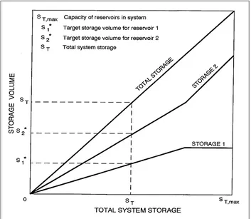
WASP (Kuczera and Diment, 1988) and WATHNET (Kuczera, 1990; Kuczera, 1992). Figure 2-2 shows a typical set of target storage curves for a two-reservoir system. For a given total system storage ST at a given time-step, the target rule curves specify the storage volumes at reservoirs 1 and 2 as S1* and S2* respectively, where the sum of S1* and S2* equals to ST.

Figure 2-1. Example of a 5-Stage Urban Restriction Rule Curves. (Source: VU and DSE, 2005)

(41)

Different sets of target storage curves can be used for different months of the year. Commonly urban water supply systems with large storage capacity will use a ‘filling’ target rule curves set over the higher streamflow, lower demand months and a ‘drawdown’ set for lower streamflow, higher demand months. This helps avoid spills in the higher streamflow periods and allows water to be stored in smaller storages closer to the demand centres in higher demand periods.

Target storage curves can be determined through optimisation, however they are generally established through modeller experience and/or system limitations and requirements. They are important so that spills are avoided during filling and demand shortfalls minimised by ensuring water is available at the time and location it is required.

2.4.2.3 Other Operating Rules

Further system operating rules could also be defined through other system variables such as environmental flow releases, diversions, hydropower generation etc. These rules are derived from studies relating to river health and hydropower generation requirements undertaken by relevant environmental and power generation authorities. They are incorporated into the models through node and carrier rules and considered permanent rules in this study, hence will not considered in the sensitivity analyses in Chapters 4 and 5.

2.4.3 Required Level of Service

Potentially the most important consideration used in estimating yield is the level of service required from the system. Also called the security of supply, the level of service is measured using one or more security criteria and their thresholds. These system specific security criteria rules can include:

• Reliability of supply – the percentage of time-steps in which restrictions are not

implemented.

• Worst severity restriction stage – the worst severity restriction stage permissible.

• Maximum consecutive restriction period – the maximum consecutive number of time steps that restrictions are allowed to be imposed on demand.

(42)

The tolerance levels of the security criteria or thresholds are determined from the acceptance of the end water users but mostly from the requirements and risks of the system and its management. That is, although the public may accept lenient performance thresholds the water authorities may adopt strict rules to avoid system failures. They are therefore generally determined by the decision makers with respect to the risk of system failure and future supply security, with some consideration given to the public opinion.

2.5 Estimation of Yield

Given the definition of yield in Section 2.4, for this study yield is synonymous with the maximum average annual demand a certain system can supply. Simply, the yield is the largest volume of water that can be supplied, on average, over a given period, without system failure.

Yield is commonly estimated by increasing or decreasing the Average Annual Demand (AAD) until the accepted level of service is almost violated. This is done using a computational water supply system model that simulates the specific water supply system that incorporates streamflow variability, operating rules and demand pattern. Throughout this study, the yield estimate was determined using such a heuristic iterative procedure which is common within the water resources industry (See SKM, 2003 for an application by the Sydney Catchment Authority). REALM is commonly used in yield estimation of urban water supply systems (SKM, 2006; ANRA, 2007; Barwon Water, 2007). Several simulations are required to converge sufficiently to the final yield estimate of the system under a specific system realisation. Within the sensitivity analysis used in this study (See Chapters 4 and 5) each yield estimate is a result of a different system realisation which includes a different combination of randomly selected variable values, positions or states. The computational expense for each estimation of yield depends on the complexity of the system being modelled, the length of the simulation, the number of simulations required to obtain the yield estimate and the power of the computer.

Two water systems are used in this thesis. A simple, hypothetical system (based on Getting Started Example given in VU and DSE, 2005) is used as a preliminary case study in Chapter 4 and the Barwon urban water supply system (SKM, 2006) is used in Chapter 5. Both of these models are simulated using the REALM computational package.

2.6 Summary

(43)

pressures. Climate change and the increasing growth in population has put many water supply systems under immense pressure, often being required to supply a demand which is close to or exceeding its limit. Such pressures have been exerted on most Australian water supply systems, resulting in record restriction periods and in some cases the introduction of permanent water saving measures. Balancing the available supply and demand is the foremost concern for water authorities. To match demand and supply, several possibilities are available, such as; reducing demand through education and water saving measures, and increasing supply through augmentation with new water sources and by optimal management of the system, policies and rules.

The yield, the volume of water that can sustainably be supplied by a system over a given period, is a key component in the management of an urban water supply system. Therefore, its accurate estimation is necessary for correct managerial procedures and practices. Although the estimation of yield consists of a number of input variables that inherently contain uncertainty and/or a range of variability. These uncertainties may be due to lack of precise knowledge of the parameters in the physical system, an unknown optimal position of the variable or combination of the two.

(44)

(45)

Chapter 3 Sensitivity Analysis

3.1 Introduction

Urban water supply systems are subject to the three key influences that significantly affect the performance of the system, affecting the yield of the system in particular. These are the inflows and outflows of the system (e.g. rainfall, streamflow and demand), the physical characteristics of the system, and the management and handling of both. To assist in the management of a system, water authorities use computational models that are an abstraction of the physical system; an approximate representation of the actual system. This approximation includes estimations and assumptions that inherently introduce imperfections and errors into the model, leading to a degree of variability that is not present in the physical system. This modelling variability, combined with the above three key influences, influence the performance of the model to correctly match the physical system. All these elements of variability lead to uncertainty regarding the performance of the model and the model output(s); in this study the yield estimate of an urban water supply system.

If the uncertainty in the input variables of a model is reduced, then the confidence in the model performance would improve and the uncertainty in the output will consequently reduce. However, simply improving of knowledge of the input variables with the greatest amount of uncertainty may not be an efficient course in effectively reducing output uncertainty. The influence of a change in an input variable on the output must also be considered. This is known as the sensitivity of a model and its output to changes in input variables. The greater aim of this project is to indicate which input variables water authorities should focus resources and research to improve the accuracy of their values so that the confidence in the yield estimate increases. This is done by identifying and quantifying the sources of variability in the yield estimate by means of sensitivity analysis. Before doing so, uncertainty and sensitivity must be understood and defined in light of water supply modelling and appropriate Sensitivity Analysis (SA) techniques selected.

(46)

in Section 3.4. This review is presented in a classification arrangement with the most significant techniques and some of their applications presented under each classification.

Section 3.5 gives a comparison of each of the reviewed techniques against a number of preferable criteria for their application to an urban water supply system model and its variables. This culminates in the selection of the most appropriate SA techniques (the Morris method, the Fourier Amplitude Sensitivity Test and the method of Sobol’), with further details regarding their algorithms, indices, advantages and disadvantages following.

A brief review of SA in water resources and hydrology is presented in Section 3.6 and finally the chapter summary is given in Section 3.7, providing a discussion of the main findings.

3.2 Sources and Typologies of Uncertainty

Ronon (1988) succinctly expressed the importance of understanding uncertainty in science and engineering with: “It seems that the only certain aspect of science is that it is uncertain”.

A degree of uncertainty surrounds everything we do: in every action, choice, decision, within all aspects of everyday life we encounter a certain degree of uncertainty. This uncertainty is assessed almost automatically, somewhat instinctively, generally as a quick qualitative risk assessment that we evaluate by drawing from past experiences. In this case, we are generally equating the uncertainty involved in an action as a lack of confidence or a lack of control over that event, considering the possible variations in the outcome that may result. Similarly, in scientific fields, uncertainty is inherent within all aspects, particularly in the field of computational modelling of a physical system. Here however, modellers and analysts equate uncertainty to a perceived lack of knowledge and/or randomness.

(47)

A computational model is an abstraction of a physical system that can be represented by Figure 3-1 (Frantz, 1995). As such, it is not only subject to the same sources of uncertainty as the real system but also a range of additional uncertainties arising from assumptions and approximations used in the formulation, parameterisation, calibration, execution and interpretation of the model. In terms of computational modelling, uncertainty can be defined as: “a potential deficiency in any phase or activity of the modelling process that is due to the lack of knowledge" (Oberkampf et al. 1998).

Real World System

Conceptual

Model Simulation Model User(s) validation verification credibility

abstraction implementation execution

Figure 3-1. Generalised Model Abstraction from Physical System (Frantz, 1995).

Burges and Lettenmaier (1975) suggests that two main sources of uncertainty exist in computational models; i) the selection of the incorrect model with correct (deterministic) parameters, and ii) the choice of correct model with incorrect, or uncertain parameters. These are often referred to as Type I uncertainty and Type II uncertainty, and almost always exist simultaneously. Within the two broad groups that Burges and Lettenmaier (1975) suggest, specific sources of uncertainty are expediently acknowledged. The identification of the sources of uncertainty of a simulation model is particularly subjective to the purpose of the application, field of investigation and the subjectivity of the analyst (Kondolf, 1995; Lewin, 2001; Ascough et al., 2008, Wheaton et al., 2008). Therefore, numerous typologies that attempt to categorise the sources of uncertainty have been developed.