Determining agent-specific rates of return in a Financial CGE model of Australia

Determining Agent-Specific Rates of Return in a

Financial CGE Model of Australia

CoPS Working Paper No. G-270, March 2017

The Centre of Policy Studies (CoPS), incorporating the IMPACT project, is a research centre at Victoria University devoted to quantitative analysis of issues relevant to economic policy. Address: Centre of Policy Studies, Victoria University, PO Box 14428, Melbourne, Victoria, 8001 home page: www.vu.edu.au/CoPS/ email: [email protected] Telephone +61 3 9919 1877

Jason N. Harris,

Jason Nassios

And

James A Giesecke

Centre of Policy Studies,

Victoria University

1 | P a g e

Determining agent-specific rates of return in a

Financial CGE model of Australia

Jason N. Harris, Jason Nassios, James A. Giesecke

Centre of Policy Studies

Victoria University

Abstract

This working paper describes the process followed to arrive at a suitable specification for the agent- and instrument-specific rate-of-return matrix for the VU-Nat financial computable general equilibrium (FCGE) model of the Australian economy. Several sources were consulted to obtain appropriate rates of return. These sources are documented in detail in this report.

Keywords: Financial CGE model; Rate of return.

2 | P a g e

Table of Contents

1

Introduction ... 3

2

Model Specifications ... 4

2.1 Bonds ... 4

2.2 Deposits and Loans ... 5

2.3 Equity ... 5

2.3.1 Setting the real return on equity ... 6

2.4 Summary of Data Inputs ... 7

2.4.1 Banks ... 8

2.4.2 Central Bank ... 9

2.4.3 Foreigner ... 10

2.4.4 Government ... 11

2.4.5 Non-Bank Financial Intermediaries (NBFI) ... 12

2.4.6 The Industry Agent ... 14

2.4.7 Superannuation Funds ... 16

2.4.8 Non-Reproducible Housing (NRH) ... 16

2.4.9 Reproducible Housing (RH) ... 19

3

Concluding Remarks ... 21

4

Tables ... 22

3 | P a g e

1

Introduction

The VU-Nat financial computable equilibrium model (FCGE) model describes the behaviour of economic agents as well as financial asset and liability agents, through a series of utility maximizing and cost minimizing equations. While fully integrated, for expository purposes it is helpful to view the FCGE model as comprising two parts:

 A traditional CGE model describing the real-side of the economy, based upon the MONASH model of the Australian economy; and

 A model of the behaviour of individual financial agents and their links with the real-side of the economy.

The real-side of the VU-Nat FCGE model is based upon MONASH, a dynamic CGE model of the Australian economy. For a detailed description of the economic mechanisms in MONASH, we refer the reader to Dixon and Rimmer (2002). Real-side CGE models have been used for many decades to answer diverse policy questions [Dixon and Rimmer (2016)]. They are however silent on, or treat implicitly, the question of how several important transactions are financed. For example, how is investment spending financed? How does the cost of financial capital affect the decision to invest in physical capital? Who is financing the public sector borrowing requirement (PSBR)? How is the current account deficit financed? Who decides how household savings are allocated? An important role of the financial part of the FCGE model is to answer these and related questions.

The financial part of the VU-Nat FCGE model identifies five financial instruments and eleven financial agents.1 Financial instruments are held by financial agents on their respective balance sheets. Each financial agent is concerned with both the asset and the liability/equity sides of its balance sheet. Hereafter, we refer to financial agents as “asset agents” in matters concerned with the assets side of their balance sheets and as “liability agents” in matters concerned with the liability and equity sides of their balance sheets. The core of the FCGE model is comprised of three data arrays, and a series of equations describing how the values in these data arrays change through time. The three arrays are:

1. A(s,f,d), which describes the holdings by asset agent d ϵ AA (where the set AA includes 11

asset agents, such as households, the commercial banks, etc.) of financial instrument fϵ INS (where the set INS includes 5 financial instruments recognised in the model, such as equity, loans, bonds, etc.) issued by liability agent s ϵ LA (the set LA is a bijective mapping of the set AA and also includes agents such as households, government, etc.);

2. F(s,f,d), which describes the flow of (net) new holdings by asset agent d ϵ AA, of financial

instrument f ϵ INS, issued by liability agent s ϵ LA;

1

4 | P a g e

3. R(s,f,d), which describes the power of the rate of return (i.e. one plus the rate) on financial

instrument f ϵ INS, issued by liability agent s ϵ LA, and held as an asset by agent d ϵ AA.

The data underpinning the stock and flow matrices, A(s,f,d) and F(s,f,d), was sourced from the Australian

Bureau of Statistics (ABS) Financial Accounts2, as discussed by Dixon et al. (2015). The rates of return discussed above were previously homogenous across agents in the FCGE model, with some instrument-specific inhomogeneity. This document details the process followed to obtain agent-specific rates of return, which we use to populate the rates of return matrix R(s,f,d) in the VU-Nat

FCGE model of Australia.

2

Model Specifications

As discussed, the VU-Nat model allows financial liability agents to raise financial capital using five distinct liability instruments. We used distinct methodologies to set the appropriate rates of return on each of these five instruments. In what follows, we provide a general description of this methodology for equity, bonds, and deposits/loans. Cash (representing the stock of physical currency) and Gold/SDR’s are assumed to earn zero rate of return3 in VU-Nat.

2.1

Bonds

The liability agents in VU-Nat are representative agents. For example, multiple commercial banks operate in Australia, and these banks each issue many bonds of differing maturity terms. Each bank may also possess unique credit ratings, which will also affect the rate of return they must offer on the bonds they issue. With this in mind, we constructed an index of the rates of return offered by the real-world constituents of each representative agent in the VU-Nat model. More specifically, we constructed indices of the market yields to maturity (YTM) offered by the model’s representative agents using liability-agent specific bond issuance data from two main sources. The rate of return offered by each representative agent in the model was then set to the rates of return we evaluated in our indices. In this section, we outline the data used to construct the rate of return indices.

The first source of data was used to determine the YTM on bonds issued by the foreign agent as liabilities (and purchased by domestic asset agents). Bond holding data for a global broad-market investment grade bond index [the Citigroup World Broad Investment Grade Bond Index (WorldBIG)] was selected to represent the rate of return on foreign bonds. The industry, government, banks, and NBFI agent bond YTM’s were derived using an Exchange Traded Fund (ETF) that tracked the Bloomberg AusBond (0+ Yr) Composite Investment Grade Bond Index (BlackRock iShares Core Composite Bond Index). We began this derivation by grouping each bond within the ETF (and hence the aforementioned index that is tracked by the ETF) by issuer of that bond, e.g., the Australian State and Federal Government bonds, as well as bonds issued by Australian commercial banks, NBFIs, and

2

See ABS Catalogue no. 5232.0

3

5 | P a g e

other Australian corporates. A weighted average YTM of these groupings was then calculated by weighting the YTM of each bond issue by their respective market values. The aggregate YTMs derived provided suitable representations of the rates of return an investor could expect to earn by holding a market-value weighted portfolio of bonds issued by the real-world constituents of each representative agent in the VU-Nat model. More detail regarding this approach to determining the bond YTMs is provided in section 2.4.

2.2

Deposits and Loans

Private lending agreements are typically undisclosed, and the agreed upon rates of return differ between different parties. For this reason, the data used to seed the agent-specific deposit and loan rates of return relied upon a variety of sources and some simplifying assumptions. For most deposit and loan rates in the matrix, quoted lending and borrowing rates collated by the Reserve Bank of Australia (RBA)4 were used as representative aggregates. The RBA data tracked a variety of indicative deposit and loan rates of return over time. The series were distinguished based on the scale (retail versus wholesale deposits/loans) and type (bank to business versus mortgage broker to individual). In some cases, the various series also identified multiple financial asset agents, e.g., commercial banks versus non-bank financial intermediaries, and distinguished lending rates by financial liability agent, e.g., investor, personal, and business rates were reported, while bank deposit rates offered by the major Australia commercial banks were also summarised. While much of the deposit and loan rates of return were therefore sourced from the RBA data series, we surveyed the big four commercial banks websites and utilised their owner-occupier package5 variable home loan rates to specify the applicable rate of return on housing sector debt6. In addition, the rate of return on foreign deposits was calculated as a weighted average of quoted overseas deposit rates from the U.S. Federal Reserve, European Central Bank (EBC), and Bank of England (BoE). We shall provide agent-specific detail regarding the exact method used to set deposit and loan rates of return in section 2.4.

2.3

Equity

The return on equity for a given stock can be decomposed into two main components: (i) the real return, derived by a financial asset agent from the payment of dividends or capital appreciation caused by retained earnings; and (ii) market valuation movements or price appreciation effects. When considered together, returns derived via points (i) and (ii) are the nominal rate of return on equity. To derive an appropriate agent-specific nominal rate of return on equity for VU-Nat, we began by deriving the real return on equity [point (i)] using Morningstar DATAnalysis data on earnings yields of selected S&P/ASX 200 listed corporates. This data allowed us to calculate the real returns offered by Australian-listed commercial banks, NBFIs, and Industry. These were calculated as the weighted average earnings yield of individual companies within each of the appropriate S&P/ASX 200 sectors. In order to determine an appropriate initial nominal rate of return, we then accounted

4

Sourced from http://rba.gov.au/statistics/tables/. Series from sections ‘Money and Credit Statistics’ and ‘Interest Rates’ were consulted.

5

A Package rate from the commercial banks is defined as one that is net of an annual package fee, typically A$395 per mortgage.

6

6 | P a g e

for point (ii) using an assumed rate of asset price inflation, which was set homogenously across the various financial liability agents in the model as being equal to the RBA’s medium-term target level for consumer price inflation (2.5 per cent). The FCGE model also contains a valuation term that accounts for movements in the inter-year value of equities due to asset valuation effects endogenously, and for further detail on this term we refer the reader to Dixon et al. (2015).

2.3.1

Setting the real return on equity

With regard to our approach in determining an appropriate real rate of return, Wilcox (2007) states that the earnings yield of a firm provides a reasonable approximation of the real expected return on its equity. This relationship is also evident in the constant dividend growth model derived by Gordon (1959), which related the price of a security (𝑃𝑡) to its future earnings (𝐸𝑡+1), the investor’s required

rate of return on equity (𝑘𝑒), the portion of earnings paid out to investors (𝜌) as dividends, the

portion of earnings retained by the company (1 − 𝜌), and the return earned on reinvested earnings (𝑟). When an investor buys an equity security, they effectively hold an ownership right to the earnings of that entity, whether they are distributed back to the investor in the form of dividend payments, or reinvested by the company. With this in mind, we followed Gordon’s (1959) method in deriving the required rate of return on equity:

𝑘_𝑒=𝜌𝐸𝑡+1

𝑃𝑡 + (1 − 𝜌)𝑟 (1)

Equation (1) is simply Gordon’s (1959) equation rearranged with 𝑘𝑒 now the subject. It states that an

investor’s required rate of return on equity is a function of the earnings per share paid out to an investor (𝜌𝐸_𝑃𝑡+1

𝑡 ), and the portion of earnings reinvested in the company that are assumed to grow at

a constant rate 𝑟. We then applied the assumption that the rate of return on reinvested earnings (𝑟) can be set equal to the investor’s required rate of return on equity plus a fixed margin (𝑐):

𝑟 = 𝑘𝑒+ 𝑐. (2)

Combining equations (1) and (2), the required rate of return on equity collapses to the required nominal rate of return on equity, which is a function of the earnings yield and a new margin (𝜋). 𝜋 is a function of the previously defined margin 𝑐, and the proportion (𝜌) of earnings retained. Herein, we assume that 𝜋is equal to the RBA’s medium-term target level of economy-wide consumer price inflation (2.50 per cent). Substituting equation (2) into equation (1) and taking account of the assumptions described here yields our final expression for the nominal rate of return (𝑘𝑒):

𝑘_𝑒=𝐸𝑡+1

7 | P a g e

We used real company data to set the earnings yield herein, and define these earnings yields as the real rates of return on company equity [see point (i) previously and Wilcox (2007)]. The calculation we performed can be summarised algebraically as7:

𝐸𝑎𝑟𝑛𝑖𝑛𝑔𝑠 𝑌𝑖𝑒𝑙𝑑 =𝐷𝑖𝑣𝑖𝑑𝑒𝑛𝑑 𝑌𝑖𝑒𝑙𝑑_{𝑃𝑎𝑦𝑜𝑢𝑡 𝑅𝑎𝑡𝑖𝑜} = (

𝐷𝑖𝑣𝑖𝑑𝑒𝑛𝑑𝑡 𝑆ℎ𝑎𝑟𝑒 𝑃𝑟𝑖𝑐𝑒𝑡)

( 𝐷𝑖𝑣𝑖𝑑𝑒𝑛𝑑𝑡

𝐸𝑎𝑟𝑛𝑖𝑛𝑔𝑠 𝑝𝑒𝑟 𝑆ℎ𝑎𝑟𝑒𝑡)

=𝐸𝑎𝑟𝑛𝑖𝑛𝑔𝑠 𝑃𝑒𝑟 𝑆ℎ𝑎𝑟𝑒_{𝑆ℎ𝑎𝑟𝑒 𝑃𝑟𝑖𝑐𝑒} . (4)

To elaborate, we used the Global Industry Classification Standards (GICS) to classify companies listed on the S&P/ASX 200 into a set of specialised sectors. For example, all Australian commercial banks were allocated to the Banking sector, while all other financial sector members (excluding the commercial banks) were classed as non-bank financial intermediaries (NBFIs). Of the remaining listed firms, we began by classifying them according to their Global Industry Classification Standard Level 1 (GICS1) industry classifications. We weighted the earnings yields of companies within each GICS1 sector by their respective total book-value of equity8, to arrive at the earnings yield of each GICS1 sector. In VU-Nat, the industry agent is an aggregation of all non-financial market sectors, so we performed a final weighted sum across all non-financial sectors to derive the earnings yield for the Industry agent in VU-Nat. As discussed previously, all financial data was sourced from Morningstar DATAnalysis Premium. The TABmate and GEMPACK platforms were then used to produce the weighted average earnings yields, according to equation (5):

𝑊𝑒𝑖𝑔ℎ𝑡𝑒𝑑 𝐴𝑣𝑒𝑟𝑎𝑔𝑒 𝑆𝑒𝑐𝑡𝑜𝑟 𝐸𝑎𝑟𝑛𝑖𝑛𝑔𝑠 𝑌𝑖𝑒𝑙𝑑_𝑡 =

∑ 𝐶𝑜𝑚𝑝𝑎𝑛𝑦 𝐸𝑞𝑢𝑖𝑡𝑦𝑖,𝑡

𝑆𝑒𝑐𝑡𝑜𝑟 𝐸𝑞𝑢𝑖𝑡𝑦𝑡 × 𝐶𝑜𝑚𝑝𝑎𝑛𝑦 𝐸𝑎𝑟𝑛𝑖𝑛𝑔𝑠 𝑌𝑖𝑒𝑙𝑑𝑖,𝑡

𝑛

𝑖=1 . (5)

The base year for all earnings yields was set to 2014, as it was deemed the best representation of normal business operation.9

We used different approaches to derive the equity returns of the foreign agent, superannuation funds, and the housing (reproducible and non-reproducible) agents, which we shall outline in section 2.4.

2.4

Summary of Data Inputs

In this section, we consider each financial liability agent successively and describe how we set the rate of return these agents offer on the bond, equity and deposit/loan liabilities they use to finance their activities. Where data exists and it was deemed necessary, we describe why (for a given instrument f ϵ INS) some of the financial liability agents s ϵ LA offer the various financial asset agents

d ϵ AA who hold their liabilities different rates of return. For a summary of the instrument-specific rates of return for each representative agent derived in this section, we refer the reader to Table 1 and Table 2. For brevity, we omitted the following agents from our summary tables:

7

The earnings per share data used in the Bank, NBFI, and Industry agent earnings yield calculations was inclusive of depreciation and amortization expenses. Additionally, the dividends were franked subject to each individual company’s tax policy for each relevant time period.

8

We also used total firm assets to determine the weights in this weighted sum calculation, however the resulting earnings yields were quantitatively similar.

9

8 | P a g e

 Households: Are not a liability agent in the model.

 Life Insurers: Life insurers principally issue equity as a liability. The majority of these liabilities were life insurance policies issued directly to households, or purchased by superannuation funds on behalf of households. As these policies do not yield a return on investment, we set the rate of return on all life insurance liabilities (equity, as well as insignificantly portioned bond and deposit/loan shares) to 0 per cent pa.

Instrument-specific rates of return R(s,f,d) for given asset agent d ϵ AA, and a given liability agent s ϵ

LA, are also set to zero (and omitted from our summary tables) if the instrument f ϵ INS is cash or Gold/SDR’s. Additionally, if an entry in the VU-Nat stock matrix is zero, i.e., A(s,f,d)=0 for any (s, f, d),

we set the corresponding entry in the rate of return matrix to zero also, i.e., R(s,f,d)=0 where A(s,f,d)=0.

2.4.1

Banks

All Australian listed banks were accounted for when deriving the rates of return offered by the representative commercial banking agent in the VU-Nat model. Specifically, the banks considered were:

 Australia and New Zealand Banking Group;

 Bank of Queensland;

 Bendigo and Adelaide Bank;

 Commonwealth Bank of Australia;

 National Australia Bank;

 Suncorp Group;

 Westpac Banking Corporation.

2.4.1.1

Bond liabilities raised by commercial banks

As discussed in section 2.1, the rate of return on bonds was calculated as the weighted average YTM on all Australian commercial bank debt held in the BlackRock iShares core composite bond fund. Our weighted sum considered all the bonds issued by the commercial banks listed above that were present in the fund10, and it therefore represented an average YTM across all credit ratings and maturities. The weighted average YTM was derived weighting the YTM of each commercial bank bond held by the iShares ETF, by the market value of each security as a proportion of the total market value of all commercial bank debt in the iShares ETF. All weights and yields were calculated using holdings data for the ETF provided by iShares as at 17/11/16. The average YTM we calculated was 2.56%. The rate of return offered by the commercial banks on their bond liabilities was set uniformly across all asset agents in VU-Nat.11

10

The BlackRock iShares fund contained debt issued by commercial banks outlined except for Bendigo and Adelaide Bank.

11

9 | P a g e

2.4.1.2

Bank equity liabilities

As mentioned, the rate of return offered by commercial banks on their equity liabilities was set using the weighted average earnings yield of all listed Australian commercial banks as at December 2014. Equation (4) was used to calculate the earnings yield of each bank, which was then used to derive the weighted average real rate of return on bank equity using equation (5). As outlined in section 2.3, the nominal rate of return was then derived from this real return by accounting for an assumed 2.5 per cent level of asset price inflation. This process yielded a final nominal rate of return on bank equity (𝑘𝑒𝐵𝑎𝑛𝑘𝑠) of 9.46%. The end-2014 value was chosen as the reference period, and all derivation

data was sourced from Morningstar DATAnalysis.

2.4.1.3

Bank deposit/loan liabilities

This commercial bank liability was generally comprised of deposit liabilities to Australian households, however several other asset agents held bank deposit/loan liabilities as financial assets. The asset-agent-specific rates of return on these bank liabilities are described below.

Central Bank as the asset agent

This was set to the RBA cash rate of 1.50%, as it indicated the rate charged on overnight borrowing by banks from the central bank.

All other Asset Agents (excl. banks, RH, and NRH)

The relevant rate of return on bank deposits and loans for all other asset agents was determined to be 2.05%. This was the average deposit rate offered on retail and investment deposits by Australian banks, based on data from the RBA interest rate series F4 (Retail Investment and Deposit Rates – October 2016). Retail rates were used due to there being no deposit rates specifically described as ‘wholesale’ in the RBA data. We assumed a minimum deposit size of $10,000 and a lock up period of between 19 – 36 months. We could not identify a specific deposit rate offered by banks to any of the asset agents that differed from this rate.

2.4.2

Central Bank

The central bank offers a return on exchange settlement balance (ESB) deposits held at the central bank by authorised Australian depository institutions (assumed to be the Australian commercial banks) equal to the cash rate. The current cash rate in Australia is 1.50%. A proportion of these ESB deposits are invested with the central bank in line with capital reserve requirements. Any ‘surplus’ ESBs held at the central bank by ADIs are paid an interest rate that is 25 basis points below the cash rate12. The rate of return paid by the central bank on deposits/loan liabilities was therefore set to 1.25%.

12

10 | P a g e

2.4.3

Foreigner

2.4.3.1

Bond liabilities raised by the foreigner

As discussed in section 2.1, the rate of return on foreign bonds was calculated as the yield to maturity of the Citigroup WorldBIG Index (as at 31/12/16). The relevant rate of return was 1.59%. This bond index includes sovereign bonds (national and regional government), collateralised and corporate debt securities. From a regional perspective, the index comprised of USD (50.40%), EUR (29.10%), JPY (12.28%), GBP (4.44%), CAD (0.94%), and other (2.83%, some of which are securities issued by the Australian Government and Australian corporates) denominated securities. As the Reserve Bank of Australia only holds foreign government bonds, and no corporate bonds, the YTM (as at 31/12/16) on the Citigroup World Government Bond Index (WGBI) was used as the rate of return on foreign bonds held by the central bank agent. This rate was 1.06%.

2.4.3.2

Foreigner equity liabilities

The nominal rate of return on foreign equity was derived as the earnings yield of ex-Australia global equity markets. We chose the MSCI All Country World Index (ACWI) ex-Australia13 (AUD) to represent this universe of stock markets. The MSCI ACWI index tracks the rates of return of 85% of all global equity markets, with the following regional weights: USA (55.13%), Japan (8.03%), UK (6.1%), France (3.39%), Canada (3.34%), and other (24.03%) – ‘other’ consists of 40 remaining developed and emerging economies. The earnings yield of the foreign agent’s equity was then calculated using equation (4). For the dividend yield, we relied on data from the MSCI ACWI fact sheet (from the MSCI index web page as at 30/12/2016)14, while we applied an average international market payout ratio (to be described momentarily) to derive an earnings yield for the foreigner agent. The dividend yield derived from this index was 2.45%. To determine a weighted average payout ratio, we used data on the average payout ratio between 2005-2015 of the US (48%), UK (60%), Japan (57%), Europe (55%), and Canada (52%), which were weighted using the holdings weights of the MSCI ACWI as summarised on the index fact sheet (the payout ratio calculated was 0.504). The international payout ratios were obtained from Bergmann (2016). Using this data, equation (4) produced an earnings yield of 4.86%. The most recently recorded global inflation rate of 1.44% per annum15 was then added to the rate to produce a nominal rate of return on foreign equity (𝑘𝑒,𝐹𝑜𝑟) of 6.30%.

2.4.3.3

Foreigner deposit/loan liabilities

To determine the appropriate rate of return on foreign deposits and loans, we began by investigating the asset agent ownership shares for deposit and loan liabilities raised by the foreigner using the VU-Nat financial stock database A(s,f,d). Our analysis showed that 91% of Australian-owned

foreign deposit/loan liabilities were financial assets of the Australian banks (50%), Australian industry (37.5%) and Australian NBFIs (3.6%). We conjectured that the majority of foreign deposit and loan liabilities owned by Australian financial asset agents were foreign direct and portfolio

13

Ex-Australia means that this index excludes all Australian equity markets.

14

This can be found at: https://www.msci.com/documents/10199/dc13f9fb-9c7c-45cc-a6e5-c298ddad5f34

15

11 | P a g e

investment debt, i.e., loans by Australian companies to offshore subsidiaries, lending to foreign companies, and also deposits into foreign financial institutions by domestic agents.

Banks as asset agents

As domestic commercial banks provide deposit services to other financial agents, we made a simplifying assumption that foreign deposit/loan liabilities held by Australian commercial banks as financial assets consisted mainly of loans to foreign firms (as opposed to deposits held as financial assets by Australian commercial banks). As such, the relevant rate of return on bank loans to the foreign agent by Australian commercial banks was set equal to the weighted average interest rate on business credit outstanding on loans from Australian banks (4.30%). This was sourced from RBA statistical series F5 (effective date: September 2016).

Industry, NBFI, and Other asset agents

To determine the rate of return on foreign agent deposit/loan liabilities held as assets by other (non-bank) financial asset agents in the model, we assume that these stocks were mainly domestic agent deposits at foreign bank (and other) financial institutions. To determine an appropriate weighted-average rate of return under such an assumption, we consulted the ABS International Investment Accounts (catalogue no. 5352.5) to evaluate the regional distribution of Australian foreign direct and portfolio debt stocks. The weights we used in our weighted average calculation were then set according to the regional distribution shares of Australian foreign direct and portfolio investment abroad, excluding all equity. From catalogue no. 5352.5, the USA, EU, and UK are found to account for 73% of overall non-equity Australian foreign direct and portfolio investment abroad. We therefore set the rate of return on foreign deposits and loans by taking a weighted sum of the two-year deposit rates (>$100,000) within three jurisdictions: the USA, EU, and UK. The applicable rates of return on USA, EU, and UK deposits were obtained from the US Federal Reserve, European Central Bank (ECB), and the Bank of England (BoE), using data from January 2017 in each case16_{. This}

yielded a rate of return of 0.60 per cent per annum, which was reflective of the low interest rate policies being implemented by central banks across major OECD economies abroad.

2.4.4

Government

2.4.4.1

Bond liabilities raised by the Australian government

In VU-Nat, the government agent raises bond liabilities to finance the public sector borrowing requirement. To determine the rate of return on Australian government bond liabilities, we referred once more to the holdings data for the iShares core composite Australian bond index ETF by BlackRock. The method discussed in section 2.4.1.1 was used to weight the government bond

16

USA: Federal Reserve Economic Database (www.fred.stlouisfed.org) series National Rate on Jumbo Deposits (≥$100,000): 24-month CD, not seasonally adjusted.

EU: ECB Statistical Data Warehouse (http://www.sdw.ecb.europa.eu) series Euro area Annualised agreed rate/Narrowly defined effective rate, Credit and other institutions reporting sector - Deposits with agreed maturity, Up to two years original maturity, Outstanding amount business coverage, Non-Financial corporations

12 | P a g e

holdings in the ETF and derive an appropriate weighted average YTM on Australian government bonds. Only government instruments (treasury and government related) were included, while the weights were based on the market value of government bonds in the index as at 17/11/16. The rate of return calculated was 2.30%, which was of similar order to the prevailing 10-year government bond yield (2.79% as at December 2016)17.

2.4.4.2

Australian government equity liabilities

The rate of return on government equity was set to zero. These liabilities were held as assets by Australian households, and we conjectured that they largely comprised of transfer payments, taxation concessions, and other non-investable financial assets.

2.4.4.3

Australian government deposit/loan liabilities

Rate of return data on asset-agent-specific non-bond government borrowings were not available, and so we assumed that these borrowings were short-term in nature. Thus, the applicable rate of return was the short-term government borrowing rate. The Australian Office of Financial Management (AOFM) was consulted to determine the rate of return paid by the Australian government on short-term debt. The weighted average yield on the zero-coupon Treasury note maturing 28/04/17 was chosen as the appropriate rate, representing a borrowing term of 3 months. This was 1.65% (as published on cbonds.com18), which was also consistent with the Treasury bond (4.25% coupon, maturing 21/07/17) yield of 1.67%19.

2.4.5

Non-Bank Financial Intermediaries (NBFI)

In setting the rates of return on the various financial liabilities issued by the non-bank financial intermediary sector, we relied on balance sheet data for those NBFI corporates that are listed on the S&P/ASX 200. We identified twenty companies in this benchmark that could be classified as NBFI’s. The twenty companies are summarised below:

 AMP Limited

 ASX Limited

 BT Investment Management

 Challenger Limited

 Credit Corp Group

 CYBG PLC

 Eclipx Group

 Flexigroup Limited

 Genworth Mortgage Insurance Australia

 Henderson Group PLC

 Insurance Australia Group

17

Retrieved from RBA series F2.1 – Capital Market Yields. Series ID FCMYGBAG10.

18

See http://cbonds.com/emissions/issue/279943

19

13 | P a g e

 IOOF Holdings Limited

 Macquarie Group

 Magellan Financial Group

 Medibank Private Limited

 OFX Group

 Perpetual Limited

 Platinum Asset Management

 QBE Insurance Group

 Steadfast Group

2.4.5.1

Bond liabilities raised by the NBFIs

The YTM for NBFI bond liabilities were set using the weighting method described in section 2.1. We used data for the set of Australian NBFI bonds (issued by the twenty companies above) that were tracked by the BlackRock iShares core composite bond fund as at 30/11/2016. The benchmark tracked three such securities, issued by Macquarie Bank and AMP Capital. The weighting procedure then produced a weighted average YTM of 3.33% for these securities.

2.4.5.2

NBFI equity liabilities

The return on NBFI equity was calculated in the same manner as the equity liabilities issued by the commercial banks (for a general description of the approach we followed, see section 2.3.1). The earnings yield of each individual NBFI firm identified above was calculated using equation (4). Then, a weighted average earnings yield calculation was performed for the NBFI agent using TABmate, GEMPACK, and the formalism in equation (5). As for the commercial banks, we used the book-value of company equity to weight the earnings yields of each of the twenty NBFI constituent companies in our sample. This produced a weighted average earnings yield of 6.21%, which was then inflated by the RBA’s medium-term inflation target of 2.50%. Inclusive of the consideration of the inflation rate, the nominal rate of return on the NBFI agent’s equity (𝑘𝑒𝑁𝐵𝐹𝐼) was 8.71%. Our calculations relied on

financial data from Morningstar DATAnalysis Premium, while the earnings yield was based on reported earnings for 2014.

2.4.5.3

NBFI deposit/loan liabilities

14 | P a g e

Banks and the Central Bank as asset agents

Private lines of credit from commercial banks, e.g., such as those used to finance acquisitions that are not funded using equity or bonds, or general short-term borrowing for daily operations, were assigned a rate of return equal to the weighted average interest rate on business credit outstanding on loans from banks (4.30%). This was sourced from the RBA statistical series F5 (effective date: September 2016). The RBA cash rate (1.50%) was set as the applicable NBFI borrowing rate from the RBA.

Industry Agents, Foreigners, and Others (excl. NBFI, RH, and NRH)

The industry and foreign agents accounted for approximately half of loans to/deposits invested at NBFIs in the VU-Nat financial stock database. We hypothesised that General Certificates of Deposit (CDs) were the likely financial instrument backing these liabilities. We consulted the list of authorised depository institutions (ADIs) on the Australian Prudential Regulation Authority (APRA) website (as at 20/12/16)20, and identified that AMP Group and Macquarie Group offer business banking services through two wholly-owned subsidiaries, AMP Bank and Macquarie Bank. To determine an appropriate rate of return on NBFI deposit liabilities owned as financial assets by the industry agent, foreigner, and other (excl. banks, CB, and housing agents) agents, we took a simple average of interest rates offered on the AMP business ‘Cash Manager’ (1.50% pa) and Macquarie Bank ‘Guarantee Express’ (0.50% pa) accounts. This resulting rate of return was 1.00%.

2.4.6

The Industry Agent

We evaluated suitable rates of return for the liabilities that the representative Industry agent used to fund non-residential physical capital formation, using a modified form of the approach outlined in section 2.4.5 for the representative NBFI agent. To elaborate, we consulted a database of companies currently listed on the S&P/ASX 200 to identify firms that comprise approximately 73% of the total market capitalisation of each non-financial GICS1 sector21 (as at 01/11/16). Balance sheet data for each company was obtained using Morningstar DATAnalysis Premium. This data was then aggregated across each company to yield representative rates of return on financial liabilities at the GICS1-industry-level, i.e., we used the weighting procedures discussed previously to derive the rate of return for the liabilities issued by each GICS1 sector by aggregating over liabilities issued by each sector’s constituent companies. For example, the YTM of bonds issued by the Industrials sector was determined by aggregating the YTM on bonds issued by its constituents, e.g., Asciano, that are tracked by the Bloomberg AusBond (0+ Yr) Composite Investment Grade Bond Index. Next, we aggregated the rates of return for each financial instrument across the GICS1 industries, and arrived at the rate of return the representative industry agent offered on the relevant financial liabilities it raised to fund non-residential physical capital formation in the model. This two-stage approach to the aggregation procedure facilitates further model development, specifically the disaggregation of

20

See http://www.apra.gov.au/adi/pages/adilist.aspx

21

15 | P a g e

the representative industry agent into its GICS1 constituents. This development will be discussed in follow up working papers, and is not considered herein. The firms that we used to derive our representative rates of return represented 48% of the S&P/ASX 200 index by market capitalisation (with the financial sector that was studied using a similar approach in sections 2.4.1 and 2.4.5 making up an additional 35% of the S&P/ASX 200 index).

2.4.6.1

Bond liabilities raised by the industry agent

The rate of return on the industry agent’s bond liabilities was determined using the approach described in section 2.1. Non-financial corporate bonds of Australian companies held in the iShares composite bond ETF were firstly classified as per their GICS1 sector. The Consumer Discretionary, Consumer Staples, Energy, Industrials, Materials, Real Estate Investment Trust (REIT), Telecommunications, and Utilities sectors featured in the ETF bond holdings. There were no Information Technology sector bond holdings.

Next, the YTMs on each of the bonds, within each GICS1 sector, were weighted by their market value (as a proportion of all Australian non-financial corporate bond liabilities raised by each sector), to produce a set of GICS1-sector bond YTMs. These sector aggregates were finally aggregated across all GICS1 sectors to produce the VU-Nat model industry agent bond YTM of 3.41%22.

2.4.6.2

Industry agent equity liabilities

To determine the earnings yield on Industry equity we first aggregated the company-specific earnings yields within each of the nine GICS1 sectors in our sample. This produced a set of representative earnings yields for each GICS1 sector. As depicted algebraically in equation (6), these sector-specific earnings yields were then aggregated (this time by weighting each GICS1 sector earnings yield by the GICS1 sector aggregate stock of equity liabilities) to produce an earnings yield for the (single) representative Industry agent.

𝐼𝑛𝑑𝑢𝑠𝑡𝑟𝑦 𝐴𝑔𝑒𝑛𝑡 𝐸𝑎𝑟𝑛𝑖𝑛𝑔𝑠 𝑌𝑖𝑒𝑙𝑑_𝑡 =

∑ 𝑆𝑒𝑐𝑡𝑜𝑟 𝐸𝑞𝑢𝑖𝑡𝑦𝑖,𝑡

𝑁𝑜𝑛 𝐹𝑖𝑛𝑎𝑛𝑐𝑖𝑎𝑙 𝑆𝑒𝑐𝑡𝑜𝑟𝑠 𝑇𝑜𝑡𝑎𝑙 𝐸𝑞𝑢𝑖𝑡𝑦𝑡× 𝐶𝑜𝑚𝑝𝑎𝑛𝑦 𝐸𝑎𝑟𝑛𝑖𝑛𝑔𝑠 𝑌𝑖𝑒𝑙𝑑𝑖,𝑡

𝑛

𝑖=1 . (6)

The real rate of return derived from this two-stage weighted average calculation was then adjusted to account for our assumed rate of domestic asset price inflation (see section 2.3), producing our final nominal rate of return (𝑘𝑒,𝐼𝑛𝑑) of 11.05% for Industry equity liabilities.

22

16 | P a g e

2.4.6.3

Industry agent deposit/loan liabilities

To determine the rate of return on Industry deposit and loan liabilities, we departed from the two-stage aggregation procedure and relied on RBA data for business borrowing rates. From the VU-Nat financial database, we noted that 65% of Industry deposit/loan liabilities were held as financial assets by the Australian commercial banks. Because the majority of industry loans are therefore sourced from Australian commercial banks, the rate of return on Industry loan liabilities was set equal to the weighted average interest rate on total outstanding bank credit to businesses reported by the RBA (Statistical series D8 – Bank Lending to Business, Selected Statistics). The rate of return reported by this series was 4.30% (September 2016). While the foreigner was the next most significant source of loan finance for Australian Industry, because these borrowings are either private credit lines or foreign direct investment via loan finance (and the rates of return are not formally discussed), no data was available to set a rate of return on foreign borrowing by industry. We therefore assigned the rate of 4.30% uniformly, i.e., all financial asset agents received a rate of return of 4.30% for loans to Australian Industry.

2.4.7

Superannuation Funds

Superannuation funds do not raise bond finance, and so we set the rate of return on bond liabilities by superannuation funds in Australia to zero. Regarding superannuation fund equity liabilities, these liabilities must offer a rate of return equal to the rate of return earned by superannuation funds on their underlying financial asset holdings (less management fees and fund expenses). This rate was set using the annual industry-wide rate of return for Australian superannuation entities with more than four members (APRA, 2016). The effective annual rate of return by Australian superannuation funds (calculated as the geometric product of the last four recorded quarterly rates of return to September 2016, after expenses and tax) was 7.40%. The ABS 5352.0 financial account data (and thus the VU-Nat financial stock database) also showed that a very small share of the liabilities raised by superannuation funds were term deposits. To set an appropriate rate of return on these liabilities, we chose a representative superannuation fund agent that offered term deposits as an investment option to its members – the Newcastle Permanent Building Society (NPBS) Superannuation fund. Using data from NPBS as at 1 July 2016 (and accounting for a 15% investment tax), the rate of return for deposit liabilities raised by superannuation funds was set at 2.59%.

2.4.8

Non-Reproducible Housing (NRH)

VU-Nat introduces two artificial financial agents who raise equity finance (from households) and loan finance (from various financial intermediaries) to fund the nation’s residential housing stock. By assumption, the NRH agent manages the stock of established properties considered inner city or ‘middle-regional’ (as defined by the Real Estate Institute of Victoria23). This stock cannot be reproduced, and net investment in the NRH housing stock is therefore zero. Nevertheless, the existing stock must be financed, and rates of return on the equity and debt liabilities raised by the

23

17 | P a g e

NRH agent must be set accordingly. The specific methods used to derive the rates of return for this agent are discussed below.

2.4.8.1

NRH equity liabilities

Data

Rental yields for the Victorian housing market were sourced from the Real Estate Institute of Victoria (REIV), both before tax and before ongoing expenses. The REIV data for GRYs on Victorian houses is disaggregated by both the number of bedrooms in the house, y, where y ϵ {2, 3, 4}, and also the location/region of the house, x, where x ϵ {inner, middle, outer}, i.e., the GRY data supplied by REIV for houses in Victoria can be represented as a two-dimensional array 𝐺𝑅𝑌𝑥,𝑦, as shown in Table 3.

The REIV defines houses located in the: (i) ‘inner’ region as being within 10km of the Melbourne CBD; (ii) ‘middle’ region between 10-20km from the Melbourne CBD; and (iii) ‘outer’ region as being houses located more than 20km from the CBD. The regional disaggregation in the REIV data was congruent with the definition of the NRH stock in VU-Nat, which is also defined as inner- and middle-suburban housing. Because a similar level of regional disaggregation was not available from data sources that report national GRYs on housing, the REIV data served as our primary data source for determining the rate of return on NRH equity, which was set equal to a weighted average gross rental yield (GRY) of inner city and middle-suburban housing. As we shall describe, we made some allowance to adjust the Victorian GRY data to reflect the broader national housing market, by re-scaling our calculated GRYs (based on REIV data) to account for scale differences between Victorian and national average GRYs for housing24.

Method

As discussed, the NRH sector in VU-Nat is assumed to consist of established inner-city and mid-suburban houses (as distinct from outer-mid-suburban houses, and units across all three regions, which will be discussed in section 2.4.9.1). To determine a rate of return on equity for these properties, we first evaluated an average GRY for both inner and middle-suburban houses using the REIV data (summarised in

Table 3

), by weighting the 2, 3 and 4-bedroom GRY in each region using national data from the ABS25 on the number of bedrooms per dwelling. This weighting is summarised by equation (7) below:

𝑊𝑒𝑖𝑔ℎ𝑡𝑒𝑑 𝐴𝑣𝑒𝑟𝑎𝑔𝑒 𝐺𝑅𝑌_𝑥 = ∑ [ (𝑁𝑜.𝑜𝑓 𝐴𝑢𝑠𝑡𝑟𝑎𝑙𝑖𝑎𝑛 𝑑𝑤𝑒𝑙𝑙𝑖𝑛𝑔𝑠 𝑤𝑖𝑡ℎ 𝑦 𝑏𝑒𝑑𝑟𝑜𝑜𝑚𝑠)𝑥

(𝑇𝑜𝑡𝑎𝑙 𝑁𝑜.𝑜𝑓 𝐴𝑢𝑠𝑡𝑟𝑎𝑙𝑖𝑎𝑛 𝑑𝑤𝑒𝑙𝑙𝑖𝑛𝑔𝑠 𝑤𝑖𝑡ℎ 2,3,𝑎𝑛𝑑 4 𝑏𝑒𝑑𝑟𝑜𝑜𝑚𝑠)𝑥×

3 𝑦=1

(𝐺𝑅𝑌𝑥,𝑦)]. (7)

24

The national data was sourced from CoreLogic Hedonic Home Value Index (January 2017) for the quarter to December 2016. Accessible at

https://www.corelogic.com.au/resources/pdf/indices/indices-release/2017-01-CoreLogic-Home_Value_Index.pdf. This data is not disaggregated into inner-, middle- and outer-suburban regions of the nation’s capital cities, but does provide averages for the GRY’s by capital city.

25

Data: 2011 Census QuickStats – Dwelling Structure

18 | P a g e

Next, an average GRY for Victorian NRH is then calculated by weighting each region’s average GRY, by the area of each region. For simplicity, we assume each region is circular and summarise our weighting procedure in equation (8):

𝑊𝑒𝑖𝑔ℎ𝑡𝑒𝑑 𝐴𝑣𝑒𝑟𝑎𝑔𝑒 𝐺𝑅𝑌_𝑁𝑅𝐻 = ∑ [ 𝐴𝑟𝑒𝑎𝑥

𝑇𝑜𝑡𝑎𝑙 𝐴𝑟𝑒𝑎× (𝐺𝑅𝑌𝑥)] 2

𝑥=1 . (8)

To elaborate on equation (8), the REIV classifies the inner region as lying within a radius of 10km of the Melbourne CBD. As the radius is uniform, this traces out an area of:

𝐴𝑟𝑒𝑎_{𝑖𝑛𝑛𝑒𝑟}= 102_{𝜋 = 314.16𝑘𝑚}2_{. (9)}

Based on the REIV classification, the middle region is concentric with the inner region, and extends to a radius of 20km from the CBD. The area of the middle region is therefore given by the area of a circle with a radius of 20km (calculated in the same manner as above), less the area of the inner region. Weighting the average GRY of the inner and middle regions in this way, yields a GRY for Victorian NRH of:

𝐺𝑅𝑌_𝑉𝑖𝑐 = 2.71%. (10)

Finally, we accounted for differences between GRYs in Victoria and the national housing market, by re-weighting GRYVic by the national-average GRY for housing relative to the reported GRY for Melbourne by CoreLogic, as shown in equation (11):

𝐺𝑅𝑌_𝑁𝑅𝐻= 𝐺𝑅𝑌_𝑉𝑖𝑐×_{𝑀𝑒𝑙𝑏𝑜𝑢𝑟𝑛𝑒 𝐻𝑜𝑢𝑠𝑒 𝐺𝑟𝑜𝑠𝑠 𝑅𝑒𝑛𝑡𝑎𝑙 𝑌𝑖𝑒𝑙𝑑 𝑅𝑒𝑝𝑜𝑟𝑡𝑒𝑑 𝑏𝑦 𝐶𝑜𝑟𝑒𝐿𝑜𝑔𝑖𝑐}𝑁𝑎𝑡𝑖𝑜𝑛𝑎𝑙 𝐻𝑜𝑢𝑠𝑒 𝐺𝑟𝑜𝑠𝑠 𝑅𝑒𝑛𝑡𝑎𝑙 𝑌𝑖𝑒𝑙𝑑 𝑅𝑒𝑝𝑜𝑟𝑡𝑒𝑑 𝑏𝑦 𝐶𝑜𝑟𝑒𝐿𝑜𝑔𝑖𝑐. (11)

We thus arrived at our final rate of return on NRH equity of 3.11%.

2.4.8.2

NRH deposit/loan liabilities

Banks and Foreign Agent

We set the rate of return on non-reproducible residential property loans to 4.53%, for all loans sourced from Australian commercial banks and the foreigner. This was derived from the standard variable home loan rate quoted by the major Australian commercial banks, for loans with a value >$750,000. For simplicity, we took a simple average (mean) of the mortgage rates offered by the big four commercial banks, based on data from 05/01/17.

NBFI, Industry, and Other Agents

19 | P a g e

series, we identified that the appropriate rate of return on NBFI (this included NRH borrowing from the industry, superannuation, and life insurer agents) loans is 4.15%.26

2.4.9

Reproducible Housing (RH)

In the same way that the NRH agent is responsible for financing the nation’s existing (non-reproducible) housing stock, the reproducible housing agent manages new investment in reproducible residential housing, e.g., housing that is located a greater distance from the central business district of their respective state/region in urban fringe developments, and all new units/apartments. To set the rates of return offered by the RH agent, we focused on the GRY for the ‘outer-suburban’ housing stock (see our description of the inner-, middle- and outer-suburban housing stock in section 2.4.8.1), and all units/flats in Australia27.

2.4.9.1

RH equity liabilities

Gross Rental Yield for Outer-Suburban Houses

A similar method to the one described in section 2.4.8.1 was used to calculate the rate of return on equity paid by the RH agent. Because the RH stock is comprised of outer-suburban houses and units across all regions, we began by determining an average rate of return on outer-suburban houses. Once more, we relied upon GRYs for outer suburban houses of 2, 3 and 4 bedrooms sourced from the REIV, which were weighted using the procedure in section 2.4.8.1 and equation (7). Using equation (7), we arrive at a weighted average GRY for outer-suburban houses in Victoria

𝐺𝑅𝑌_{𝑉𝑖𝑐,𝑜𝑢𝑡𝑒𝑟}= 3.72%. Finally, we account for differences between the Victorian and national housing markets using equation (11), yielding an estimated GRY for outer-suburban housing in Australia 𝐺𝑅𝑌𝐴𝑢𝑠,𝑜𝑢𝑡𝑒𝑟 = 4.27%.

Gross Rental Yield for Units

Because all units, i.e., units in inner-, middle- and outer-suburban regions, are classified as reproducible housing in VU-Nat, we relied upon the national median GRY for units reported by the CoreLogic Hedonic Home Value Index, which was 4.10% as at end December 2016.

RH Agent Gross Rental Yield

Next, to calculate 𝐺𝑅𝑌𝑅𝐻 we evaluated a weighted average of the outer-suburban housing and unit

GRYs. Determining the appropriate weights involved a two-stage process. First, we sourced data on the total number of building approvals28 in Australia for the most recent three months to November 2016. This data served as a proxy that allowed us to estimate the proportion of outer-suburban

26

Some other agents, e.g., superannuation funds, life insurers, and Industry, also finance a very small share of NRH housing loans. For simplicity, we allocated the rate of return on the NRH loans owned by these agents according to the rate of return offered on NBFI loans.

27

Defined by the ABS as dwellings in blocks of flats, units or apartments. These dwellings do not have their own private grounds and usually share a common entrance foyer or stairwell. Definition from series 2901.0 Census Dictionary – Dwelling Structure.

28

20 | P a g e

houses relative to the proportion of units that make up Australia’s reproducible housing stock, in the following way. Firstly, we assume that the stock of units in Australia can be proxied by the Total Number of Dwellings Approved - Excluding Houses data in ABS series no. 8731.06, and that the stock of outer-suburban houses can be proxied by the Total Number of Houses Approved in all Sectors (also see ABS series no. 8731.06). Each respective building approval count (and house/unit number proxy) is then multiplied by the national median price for a house/unit, sourced from the CoreLogic Hedonic Home Value Index. Dividing the (proxy) value of Australian reproducible houses and the (proxy) value of Australian units by the total value of Australia’s reproducible housing stock yields the following weights:

 55.87% for houses, and

 44.13% for units.

We then used these to weight 𝐺𝑅𝑌𝐴𝑢𝑠,𝑜𝑢𝑡𝑒𝑟 = 4.27% and 𝐺𝑅𝑌𝑈𝑛𝑖𝑡𝑠 = 4.1% to derive 𝐺𝑅𝑌𝑅𝐻, the

return on equity paid by the RH agent, using equation (12):

𝐺𝑅𝑌𝑅𝐻= (𝐺𝑅𝑌𝑂𝑢𝑡𝑒𝑟× 0.5587) + (𝐺𝑅𝑌𝑈𝑛𝑖𝑡𝑠× 0.4413) = 4.20%. (12)

2.4.9.2

RH deposit/loan liabilities

Banks and Foreign Agents

As for the NRH agent, an overwhelming majority of RH loans and deposits were financed by Australian commercial banks. Consistent with the methodology used to derive the NRH borrowing rate from banks and foreigners, the bank and foreign borrowing rate for reproducible housing was derived using the standard variable bank home loan rate for loans between $250,000 - $750,00029. We reduced the principal value relative to the value we used to derive the NRH housing loan rate of return, to reflect the fact that outer-urban fringe house prices (and the price of units/apartments) are typically lower than the price of inner-city (non-reproducible) housing. The quoted mortgage rates obtained from the big four banks were aggregated using a simple average across Commonwealth Bank, Westpac, NAB, and ANZ (rates applicable as at 05/01/17). This yielded a required rate of return on bank loans to the RH agent of 4.62%, at a small premium to the NRH yield.

Industry, NBFIs, and Other Agents

Like the NRH agent, some RH loans are also sourced from NBFIs, the industry agent, superannuation funds, and life insurers. The rate of return on RH loans from these agents was set to 5.00%, using the mortgage manager standard lending rate quoted in the Reserve Bank of Australia (RBA) statistical series F5 (Indicator Lending Rates - December 2016). This rate exceeded the NRH equivalent rate by 85 basis points.

29

21 | P a g e

3

Concluding Remarks

The purpose of this project was to set the rates of return financial agents offer on the equity, bond, deposit/loan, cash, and Gold/SDR liabilities they raise in the VU-Nat FCGE model of Australia. At this point, the rates of return currently in the model can be set to reflect the values derived in this report, which are indicative of the market financing costs faced by Australian financial liability agents. In future work, we plan to extend this presented in three directions:

 Rates of return on housing equity were founded on simplifying assumptions – primarily due to insufficient availability of data. For example, we generalized house GRYs derived from the Victorian housing market, to a national Australia level. Our intention is to adjust the method herein to take account of national rental yield data.

 Lending rates to industry and financial agents are approximations based on statistical-aggregate rates provided by the RBA. With some clarity on personal lending agreements, e.g., sourced from public disclosure documents, we may be able to provide more nuanced asset-agent-specific rates of return on industry loans.

 Foreign financial instrument returns were based on returns provided by funds that track global benchmark indices. More clarity on agent-specific foreign direct or portfolio investments, and the regional exposures of the foreign investments made by various Australian financial asset agents, e.g., we may ask which countries Australian superannuation funds purchase equity liabilities from (developed versus emerging market breakdowns may be useful here), would allow us to specify the rate of return earned by domestic investors on foreign investments with greater accuracy.

 As it stands, the rate of return for the industry agent is an aggregate of nine GICS1 industry sectors. In the future we wish to disaggregate the stock and flow matrices in the model, in order to utilize the GICS1-level rates of return derived herein.

22 | P a g e

4

Tables

Table 1: Rates of return offered by the various liability agents in VU-Nat on their equity and bond liabilities. All financial asset agents are offered identical rates of return on the bond and equity liabilities raised by financial liability agents in the model, and we thus suppress the financial asset

agent dimension in this table.

30

The RBA typically holds a large majority of foreign government bonds, rather than corporate debt. Consequently, we used the YTM of a broad global index of Government Bonds (the Citigroup WGBI) to set the YTM of Foreign Bonds held by the Central Bank agent in VU-Nat. This rate of return is detailed in section 2.4.3.1.

Liability Agent Bonds Equity

Banks 2.56% 9.46%

Central Bank n/a n/a

Foreigners 1.59%30 6.30%

Government 2.30% n/a

Industries 3.41% 11.05%

Non-Bank Financial Intermediaries

3.33% 8.71%

Superannuation Funds n/a 7.40%

Non-Reproducible Housing

n/a 3.11%

23 | P a g e

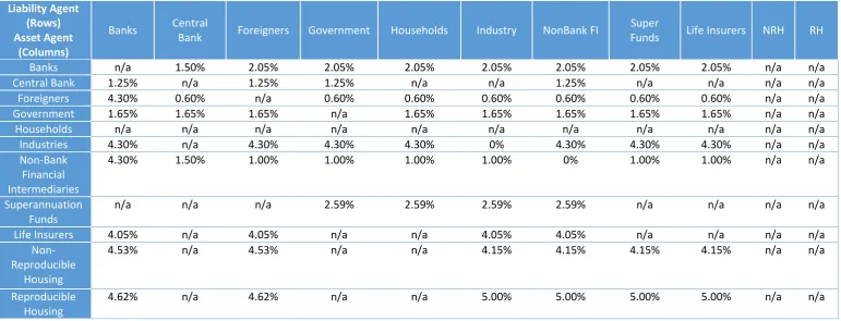
Table 2: Rates of return offered by the various liability agents in VU-Nat on their deposit and loan liabilities. For this financial instrument, there was sufficient data to disaggregate the rate of return by financial asset agent

Liability Agent (Rows) Asset Agent

(Columns)

Banks Central

Bank Foreigners Government Households Industry NonBank FI

Super

Funds Life Insurers NRH RH

Banks n/a 1.50% 2.05% 2.05% 2.05% 2.05% 2.05% 2.05% 2.05% n/a n/a

Central Bank 1.25% n/a 1.25% 1.25% n/a n/a 1.25% n/a n/a n/a n/a

Foreigners 4.30% 0.60% n/a 0.60% 0.60% 0.60% 0.60% 0.60% 0.60% n/a n/a

Government 1.65% 1.65% 1.65% n/a 1.65% 1.65% 1.65% 1.65% 1.65% n/a n/a

Households n/a n/a n/a n/a n/a n/a n/a n/a n/a n/a n/a

Industries 4.30% n/a 4.30% 4.30% 4.30% 0% 4.30% 4.30% 4.30% n/a n/a

Non-Bank Financial Intermediaries

4.30% 1.50% 1.00% 1.00% 1.00% 1.00% 0% 1.00% 1.00% n/a n/a

Superannuation Funds

n/a n/a n/a 2.59% 2.59% 2.59% 2.59% n/a n/a n/a n/a

Life Insurers 4.05% n/a 4.05% n/a n/a 4.05% 4.05% n/a n/a n/a n/a

Non-Reproducible

Housing

4.53% n/a 4.53% n/a n/a 4.15% 4.15% 4.15% 4.15% n/a n/a

Reproducible Housing

24 | P a g e

No. of Bedrooms

Region

2 3 4 Inner 2.80% 2.60% 2.30%

Middle 2.70% 2.90% 2.60%

Outer 3.90% 3.80% 3.50%

Table 3: House Gross Rental Yields by Region (𝒙) and Number of Bedrooms (𝒚) from Real Estate Institute of Victoria.

5

References

APRA, Statistics: Quarterly Superannuation Performance Report, Australian Prudential Regulatory Authority, September 2016.

Bergmann, M., The Rise in Dividend Payments. Reserve Bank of Australia, 2016

Dixon, P. B., and M. T. Rimmer, Dynamic general equilibrium modelling for forecasting and policy. A practical guide and documentation of Monash. Elsevier, 2002

Dixon, P. B., J. A. Giesecke and M. T. Rimmer, Superannuation within a Financial CGE Model of the Australian Economy. CoPS/Impact Working Paper G-253, 2015.

Dixon, P. B. and M. T. Rimmer, Johansen’s legacy to CGE modelling: Originator and guiding light for 50 years. Journal of Policy Modelling 38(3), 421–435, 2016.

Gordon, M. J. Dividends, Earnings, and Stock Prices. The Review of Economics and Statistics, 41(2), 1959, pp. 99–105, 1959.