Journal of Fluid Mechanics
http://journals.cambridge.org/FLMAdditional services for
Journal of Fluid Mechanics:
Email alerts: Click here Subscriptions: Click here Commercial reprints: Click here Terms of use : Click here
Wavefields forced by long obstacles on a betaplane
M. A. PAGE and E. R. JOHNSON
Journal of Fluid Mechanics / Volume 406 / March 2000, pp 221 245 DOI: 10.1017/S002211209900751X, Published online: 08 September 2000
Link to this article: http://journals.cambridge.org/abstract_S002211209900751X
How to cite this article:
M. A. PAGE and E. R. JOHNSON (2000). Wavefields forced by long obstacles on a betaplane. Journal of Fluid Mechanics, 406, pp 221245 doi:10.1017/S002211209900751X
Request Permissions : Click here
c
2000 Cambridge University Press
Wavefields forced by long obstacles on a
beta-plane
By M. A. P A G E1 AND E. R. J O H N S O N2
1Department of Mathematics and Statistics, Monash University, Clayton 3168, Australia 2Department of Mathematics, University College London, Gower Street,
London, WC1E 6BT, UK
(Received 29 April 1997 and in revised form 23 August 1999)
This paper presents analytical and numerical solutions for steady flow past long obstacles on aβ-plane. In the oceanographically-relevant limit of small Rossby and Ekman numbers nonlinear advection remains important but viscosity appears only through the influence of Ekman pumping. A reduced boundary-layer-type equation is derived giving the long-obstacle limit of an equation described in Page & Johnson (1990). Analytical solutions are presented or described in various asymptotic limits of this equation and compared with previous results for this or related flows. A novel technique for the numerical solution of the boundary-layer equation, based on a downstream–upstream iteration procedure, is described. Some modifications of the asymptotic layer structure described in Page & Johnson (1991) and Johnson & Page (1993) for the weakly nonlinear low-friction regime are outlined for the case of a lenticular obstacle.
1. Introduction
Finite-amplitude coastal topographic Rossby waves, or continental shelf waves, were first observed along the Australian coast by Hamon (1962, 1963, 1966) and continue (e.g. Louis, Petrie & Smith 1982; Pickart 1995; Miller, Lermusiaux & Poulain 1996) to be a typical feature of the low-frequency variability of coastal flows. Observations of dynamically similar planetary waves are more recent. Emery & Magaard (1976) infer the presence of Rossby waves from temperature fluctuations but direct observations have become common only with the availability of accurate altimeter data from the Geosat (Halliwell, Cornillon & Byrne 1991; Halliwell, Ro & Cornillon 1991; Jacobs, Emery & Born 1993; Van Woert & Price 1993) and TOPEX/POSEIDON (Schlax & Chelton 1994; Wang & Koblinsky 1995; Polito & Cornillon 1997) missions. The source of these waves might be forcing by travelling storms (Lighthill 1967) but many wave-fields appear to be associated with topographic perturbations in the form of islands or submarine ridges, with Van Woert & Price (1993) noting that Rossby wave activity represents a significant mode of mesoscale variability near the Hawaiian Islands.
Page (1993) (denoted PJ90, PJ91 and JP93 here) attempt to show how a large topo-graphic perturbation could force large-scale perturbations to an eastward flow and thus suggest that some current paths could be determined by standing Rossby waves. The analysis identifies three parameters determining the form of flow patterns in the oceanographically relevant limit of small Rossby and Ekman numbers:α, the ratio of theβ-effect to Ekman pumping destruction of vorticity;λ, the ratio of advection to Ekman pumping; andL, the ratio of the along-stream length to cross-stream width of the obstacle. Numerical solutions of the full nonlinear governing equations are given for obstacles whose aspect ratio L is of order one and interpreted by considering the first (leading-order) effects of nonlinearity on the almost-inviscid solutions for α1, following Foster (1985).
Many coastal features are, however, long compared to their cross-stream width (L1) and much analytical progress has been made by considering flows past thin obstacles (Grimshaw 1987; Grimshaw & Yi 1990, 1993; Clarke & Johnson 1997a, b). It is the purpose of the present paper to show that following these authors and confining attention to long obstacles reduces the parameter space to two dimensions, allows further analytical approximation, permits a novel, more efficient numerical solution technique and leads to an almost complete classification of flow patterns. The boundary in parameter space between unidirectional and locally-reversing flows can be completely delineated and steady stable flows with local reversals found.
The two parameters determining the flow are taken to be γ = L/α, measuring the obstacle length in terms of the Ekman decay scale of the almost-inviscid flow and b= (λ/α)1/2. The parameter b is a Rossby-wave Froude (RWF) number based
on the obstacle width. It gives the ratio of the oncoming flow speed to the phase speed of a long Rossby wave (i.e. with along-stream wavenumber near zero) with cross-stream wavelength of order the obstacle width. As in the low-Froude-number flows of non-rotating, two-dimensional stratified fluids (Chen, Rottman & Koch 1994; Baines 1995), low-RWF-number (small b) flows exhibit the analogues of upstream blocking, severe downslope winds and overturning in the lee of obstacles (see Haynes, Johnson & Hurst 1993 and Johnson & Clarke 1999 for examples in a particularly simple geometry). The analysis of Grimshaw & Yi (1990, 1993) corresponds to the large-RWF-number limit where b1 and the ratio of channel to obstacle width is of order b. They show that provided this ratio is not near a multiple ofπb the flow perturbation is linear but that near these critical values resonance with a standing Rossby wave in the channel means an obstacle can force perturbations of order the channel width, much larger than the obstacle width. The mechanism for overturning in the flows considered here thus differs from the resonance mechanism described by Grimshaw & Yi forb1 and the present study, forbof order unity and smaller, is complementary to theirs.
b
c
§5.1 In
viscid (
c<
<
1)
§5.2 W eakl
y damped (
c< <1,
b
2) §5.3 Long wavelength
(b>>1)
§4.1 Linear (b<<1)
§4.3 Nonlinear (
b~c<<
1)
§4.2 Weakly nonlinear (
b<< c<<1)
Figure 1.The various asymptotic regimes and the sections where they are considered.
2. The governing equations
2.1. The full equations
Consider a homogeneous fluid of density ρ∗ and kinematic viscosity ν∗, contained
between two infinite horizontal planes an average distance d∗ apart.† The entire
configuration is rotating at angular velocity Ω∗ about a vertical axis Oz∗ in terms of
Cartesian coordinates Ox∗y∗z∗ fixed in a frame of reference rotating with the fluid.
The lower plane is inclined at a small angle β from the horizontal so that it slopes upward in the y∗-direction. A cylindrical obstacle of cross-stream width 2`∗ and
streamwise length 2L∗ occupies the whole fluid depth in the neighbourhood of the
origin, and is aligned with its generators parallel to the axis of rotation. At some time
t∗ = 0 the fluid at large distance is set into uniform motion along lines of constant
depth at a uniform speedU∗ in the x∗-direction.
The flow can be described by five non-dimensional parameters
Ro=U∗/Ω∗`∗, E =ν∗/Ω∗d∗2, tanβ, d=d∗/`∗, L=L∗/`∗, (2.1)
the Rossby number, Ekman number, bottom slope, scaled depth and scaled obstacle length. For slow almost-inviscid flow, in which E, Ro andβ are small, the motion is two-dimensional to leading order, with horizontal velocity components given by the geostrophic relations
u=−ψy, v=ψx, (2.2) where 2ρ∗U∗Ω∗`∗ψ is the deviation of the pressure from its equilibrium value.
The evolution of the flow is governed by the equation for the vertical component of relative vorticity, ζ=vx−uy=∇2ψ,
τζt+λ(uζx+vζy) +αv+ζ= 0, (2.3) as noted in PJ90. Here t is time scaled on 1/Ω∗, with all lengths scaled on `∗ and
velocities onU∗. The parameter τ= 1
2E−1/2 is the scaled Ekman spin-up time and
α= tandE1/β2, λ= 2RoE1/2. (2.4)
Equation (2.3) follows from the full Navier–Stokes equations in the limit β →0,
Ro → 0 and E → 0 with α, λ, d and L fixed. In this limit the Reynolds number based on the obstacle width, Re = U∗`∗/ν∗ = Ro/d2E, is infinite and the flow is
effectively inviscid. The only viscous effect is through the destruction of vorticity by Ekman pumping, represented by the final term on the left-hand side of (2.3). Horizontal viscous effects are absent from the bulk of the fluid and the flow satisfies the usual inviscid impermeability conditions on solid boundaries. Vertical boundary layers within which the horizontal viscous terms are important form against solid boundaries. These layers and their possible separation from the obstacle are discussed in greater detail in both PJ90 and PJ91.
At leading order the sloping-bottom configuration is equivalent to the β-plane approximation in geophysical flows where the depth is constant and the flow is taken to be rotating at the dimensional rate 1
2(f∗+β∗y∗). The sole changes in moving to
the β-plane are to replace tanβ by β∗d∗/f∗ andΩ∗ by 1
2f∗. The Oy-direction is then
northward and Oxeastward.
Attention will be restricted to obstacles symmetric about the planey= 0, although this is not crucial to all of the subsequent analysis. Further, the steady solutions will also be taken to be symmetric about y = 0. Asymmetric steady leading-order solutions might possibly exist, as found by Cessi & Ierley (1995) in basin flow, but seem unlikely as the boundary here is an interior boundary of finite length and the ‘Island Rule’ (Pedlosky et al. 1997) requires the circulation around the obstacle to vanish. It is thus sufficient to consider flow only in y > 0 subject to the inviscid boundary condition
ψ = 0 ony=h(x/L), (2.5) wherehhas maximum value of unity and vanishes asx→ ±∞. For uniform flow far from the obstacle, the far-field condition is
∇ψ→(0,−1) asx2+y2→ ∞. (2.6)
2.2. The long-obstacle equations
This paper concentrates on steady solutions of (2.3) for long obstacles (L1) in the limit of weak Ekman pumping (α1). A reduced boundary-layer-type equation in this limit follows from (2.3) by introducing the longxscaleX=x/Land considering the weak pumping limit, α→ ∞, with
b2=λ/α and γ=L/α, (2.7)
fixed. Then (2.3) shows that the steady flowψ(X, y) satisfies
b2∂(ψ , ψyy)
∂(X, y) +ψX+γψyy= 0 (2.8) for y > h(X). This equation appears both in PJ90, where solutions for finite-width flow domains were noted and in PJ91, when describing ‘southern boundary layers’ in rapid flow.
In regions of the flow where (u, v)≈(1,0) the unsteady form of equation (2.8) can be linearized and has solutions of the form ψ∝exp [i(kX+ly−ωt)], with
ω¯τ=b2k−k/l2−iγ, where ¯τ=τγ. (2.9)
greater part of the steady disturbance in the weakly damped case will be ‘above’ (i.e. abreast of) the obstacle (in |X| 6 1, ˜y > 0). The flow close to the obstacle is not precisely uniform and so there is some slight propagation of waves both up- and downstream. Transient parts of the disturbance (which have other wavenumbers) can also affect the eventual steady-flow pattern away from the obstacle.
The parameter b measures the wavelength of a typical standing Rossby wave relative to the obstacle width. In dimensional variables the wavelength of a long Rossby wave that stands in an oncoming flow is given by (U∗/β∗)1/2 on aβ-plane or
(U∗d∗/2Ω∗tanβ)1/2 here. Non-dimensionalized on the obstacle width this gives
b= (U∗d∗/2Ω∗tanβ)1/2/`∗,
the dimensional expression of (2.7). Similarly, in dimensional variables
γ=L∗d∗E1/2/[`∗2tanβ].
It is shown in Foster (1985) and PJ90 that in slow flow the influence of an obstacle of width`∗ extends a distanceα`∗ upstream. Thusγgives the ratio of the streamwise
extent of the obstacle to the upstream-influence decay scale. Increasing γ withb con-stant corresponds to decreasing viscosity with other dimensional quantities fixed while increasing b with γ constant corresponds to increasing speed with other quantities fixed.
The boundary condition on (2.8) for finite-amplitude topography can be conve-niently transferred to a coordinate line by introducing the Prandtl transformation ˜
y=y−h(X). In terms of (X,˜y) equation (2.8) becomes
b2∂(ψ , ψ˜y˜y)
∂(X,˜y) +ψX−h0(X)ψ˜y+γψ˜y˜y = 0, (2.10) with boundary conditions
ψ(X,0) = 0 and ψ(X,˜y)∼ −˜y−h(X) as ˜y→ ∞. (2.11) It is important to note that ˜v=ψX is the ‘vertical’ velocity component relative to lines of constant ˜y, while v=ψX−h0(X)ψy˜ is the same component relative to lines
of constant y. For obstacles with discontinuous gradient at X =±1 this means that ˜
v will be discontinuous at these points, with the streamlines of ψ(X,˜y) undergoing a sudden change in slope, whereas v is continuous everywhere and the streamlines are smooth when plotted against (X, y).
3. Generalband γ
3.1. Numerical technique
The longwave-equation (2.10) can be solved straightforwardly by a novel upstream– downstream iteration procedure. Consider first the case b= 0 in (2.10), which yields a parabolic partial differential equation for ψ(X,˜y). This equation can be integrated upstream, in the negative-X direction, from the uniform-flow condition at large X, subject to the boundary conditions (2.11), and for b = 0 this gives the complete solution to the problem.
Forb >0 downstream advective effects are also important and the relative vorticity
ζ =ψ˜yy˜ satisfies the equation
b2∂(ψ , ζ)
For a given streamfunction fieldψ, this is a first-order hyperbolic equation forζ and in principle can be integrateddownstreamalong each streamline to yieldζeverywhere, once a suitable upstream boundary value forζ has been specified.
The bi-directional nature of the equation, depending on whether (3.1) is solved for
ζ given theψ field everywhere, or the equivalent equation
∂(ψ , Π)
∂(X,˜y) +γψ˜y˜y = 0 (3.2) is solved for ψ given the potential vorticity field Π = b2ζ+ ˜y+h(X) everywhere,
reflects the mixed parabolic–hyperbolic character of the steady equation and suggests an iterative approach to solving the steady wave problem for b >0.
Ekman dissipation causes ζ to vanish sufficiently far upstream (in practice, over distances larger than O(1/γ)). Thus starting with an initial approximationζ0 = 0 for
the upstream vorticity at Xmin, say, and usingψ=−y˜andΠ = ˜y+h(X) as an initial approximation downstream to Xmax, say, (3.2) can then be solved numerically for ψ over the finite sub-domain Xmin 6X 6Xmax and 06y˜6˜ymax by integrating in the upstream direction. The resulting values of ψ atX =Xmin are then used to calculate updated values ofζ at that boundary and then (3.1) can be solved along streamlines to obtain improved values forζ everywhere. This process is repeated until both theψ
and ζ fields converge, in which case both (3.1) and (3.2) will be satisfied everywhere and ζ will equalψ˜yy˜ over the domain.
For the figures shown here, the numerical method for solving the parabolic equation (3.2) for ψ during the upstream sweeps was based on the Crank–Nicolson method. For the downstream sweeps, the hyperbolic equation (3.1) was solved for ζ using a semi-Lagrangian technique based on quadratic interpolation for the value ofζ on the same streamline at the previous X grid value. For streamlines entering at ˜y = ˜ymax the ‘undisturbed’ boundary valueζ = 0 was specified. All calculations shown in this paper were obtained using a non-uniform spatialXgrid, similar to that used in PJ90, typically with 256 gridpoints over−106X 610. In the ˜y-direction a stretched grid similar to that in PJ90 was used forb1 with a uniform grid used for larger values ofb, and typically 64 gridpoints were used in ˜y with ˜ymax equal to at least 40b, and often even larger for small values of γ. For small values of b an initial guess with
ψ = −˜y was used and for larger b one of the approximate solutions in §5 led to rapid convergence. The criterion used for termination of the upstream–downstream iterative process was that changes in ψ be less than 0.1% everywhere.
3.2. Streamline overturning
Clearly, the method described above for the downstream integrations can fail when there are overturned streamlines anywhere in the flow, even if this occurs only temporarily during the upstream and downstream iterations, and therefore u=−ψ˜y should be positive everywhere for reliable results. Similarly, the ‘upstream’ integrations forψ require thatΠ˜y should be positive everywhere, to ensure that (3.2) is integrated in the ‘stable’ direction. Typically, these requirements are true everywhere for all flows except those over limited ranges of values of b, and for larger values of γ they are true for all values ofb.
An ‘inviscid’ flow, with γ = 0, is a special case as (3.2) implies that the two requirements above coincide; if u= 0 at any isolated point in the flow for a certain value of bthen Π˜y must also be zero at that point. The largest value of bfor which
u= 0 anywhere in the flow forγ= 0 is referred to asbc in this paper.
0.8
0.6
0.4
0.2
0
0.2 0.4 0.6 0.8 1.0
b = 1.0
b = 0.1
b = 0.5
(a) (b)
1.5
1.0
0.5
0 0.5 1.0
c c
min Py
min u
Py <0
Figure 2. (a) Curves showing the global minima of both u and Πy as a function of γ for
b= 0.1,0.5,1.0. Note that in each case theucurves (dotted) remain positive where the Πy curves
(unbroken) cross zero, but that the two curves become closer as b increases. (b) A plot of the parameter space (γ, b) showing the approximate region whereΠy <0 somewhere in the flow, based
on the numerical calculations obtained using the method described in§3. The dots on the figure give the parameter values used for figures 3, 4, 6, 7, 8(b) and 9(a).
the same, but not necessarily identical, parameter values. For example, if γ was decreased at any fixed value ofb < bc(wherebc≈1.29 for a parabolic obstacle) then the global minima ofuand Π˜y both decreased but Π˜y often appeared to be the first to actually reach zero. To see why this occurs, consider the marginal case whereu= 0 at an isolated point in the flow and positive elsewhere, so that the streamline passing through this point is vertical. Decreasing ˜y through this point, u falls from being positive to being exactly zero, and then becomes positive again. It then follows that
ζ = −u˜y =ψ˜yy˜ is also zero at the point, and hence from (3.2) thatΠ˜y must also be zero. As a result, the ‘critical value’ ofγfor min{Π˜y}= 0 at that value ofbcan be no smaller than the ‘critical value’ for min{u}= 0, but for γ > 0 there does not appear to be any theoretical reason why these two critical values need coincide. Indeed, the numerical calculations based on the method described above, shown in figure 2(a), support this claim. At larger values of b, but still less thanbc, the curves foruandΠ˜y become closer, consistent with the two quantities being equal everywhere whenγ= 0 (see§5).
A plot of the approximate region of (γ, b) parameter space for which Πy˜ remains
positive everywhere is shown on figure 2(b), also based on the numerical solutions of (2.10) from this study. The boundary of this region cannot be found very precisely using the method described above, as the iteration for the numerical solution can diverge if the conditions are even violated temporarily during the calculations, so that in some cases it was necessary to extrapolate for the ‘critical value’ of γ at each fixedb. This was particularly true for the larger values ofb, whereγis small near the critical value.
Two of the most important features of this plot are that the boundary of the
w f
u v
_
+
_
Figure 3. Numerical solutions of the long-obstacle equations (2.8) for flow past the parabolic
obstacle (4.2) showing contours of the streamfunctionψ, vorticityζand velocity components (u, v) whenγ= 1 andb= 1. The solution is plotted over the range 06y620 and the contour intervals used are ∆ψ= 0.25, ∆ζ= 0.05 and ∆u= ∆v= 0.05.
slope is determined by a critical value of B =b/γ for flow overturning to occur in that regime. The maximum value of bfor which any overturning of the Π contours occurs whenγ= 0, is the critical valuebcfor those solutions. The solutions forγ= 0 are described further in §5. Analysis near the point γ= 0, b=bc also suggests that the curve for the critical values is a straight line in the vicinity of this point, rather than approaching the axis tangentially.
Similar plots to figure 2(b) for obstacles with other shapes have been considered by the authors, including one with h(X) = cos2πX for which the obstacle has no
discontinuity in gradient atX =±1, and these all show the same features in figure 2(b).
3.3. General properties of the flow
bγ). This wavefield is strongest abreast of the obstacle, although it is also present in both the upstream and downstream flow through the effect of standing Rossby waves.
The presence of Ekman dissipation leads to a decay in amplitude of the wavefield in both the streamwise and vertical directions. In the former case, the strength of the wavefield decays exponentially over a downstream scale of size O(b2/γ), so that
b2ζ
X+γζ ≈0
once the flow has almost returned to the uniform velocity u = 1. In the vertical direction it will be demonstrated in §5.2 that the wavefield is damped out over a length scale of O(b3/γ), or O(b2/γ) relative to the dominant vertical wavelength. In
both cases the length scale of these effects decreases as γis increased.
The vertically-propagating wavefield from the γ= 0 flow is not only modulated in amplitude by the effect of Ekman damping for small γ, but the phase of the waves also changes in y. This displaces the extrema of both u and ζ downstream with increasing yso the wavefield appears to propagate outwards in a slightly ‘off-vertical’ direction. This ‘off-vertical’ propagation can be seen in figure 3, and also in figure 12 of PJ90.
The plot of thev(not ˜v) field in figure 3 shows three sets of vertically-propagating standing waves (of wavelength 2πb). The main set, which is also clear in the vorticity plot, is forced by fluid rising over the bulk of the obstacle, but there are also two other sets of waves, narrower in the X-direction, which appear to be generated by the sudden change in slope of the obstacle at X =±1.
As was seen in PJ90, and will also be demonstrated in §4.1, the flow upstream from the obstacle for small values ofbis dominated by a blocked region, which lies principally belowy = h(0) and decays towards uniform flow over a length scale of
O(1/γ). A similar feature is also present for largerbbut for smallγthe flow pattern is periodic inyand so blocked regions appear abovey=h(0) also. This is the signature of standing Rossby waves of wavenumber k= (0,1/b) which travel upstream from the obstacle in an unsteady flow.
For large values ofγthe flow is dominated by the damping effect of Ekman suction and the streamlines follow the shape of the obstacle at every value of y, withu= 1 andζ1 everywhere, andψ≈ −˜y=h(X)−y. In this case, the disturbance extends out toy=∞ despite the very high damping.
3.4. Solutions of the full equations
For parameters where no streamlines overturn the upstream–downstream iteration process described in §3.1 gives the steady solutions efficiently. However steady solu-tions of the full equasolu-tions can still exist at parameter values at which the flow has overturned streamlines. To illustrate this, numerical solutions of full equations (2.3) (retaining terms of the formψxx in ζ), subject to the boundary conditions (2.5) and (2.6), were also calculated for this study. These were obtained using an approach similar to that described in PJ90 but for flow past the lenticular obstacle
h(x/L) =q1
4(L2+ 1)2−x2− 12(L2−1) (3.3)
for |x|< L with h(x/L) = 0 for |x| >L. This obstacle shape was chosen because it can be mapped conformally to a rectangular domain but it also reduces to (4.2) in the limit L1 used in this paper.
mapping the resulting variable-width channel to a constant-width channel and treating this simpler rectangular domain in Cartesian coordinates (x0, y0). For the lenticular
obstacle (3.3) the transformation used is
z0= 2L n
(z+L)2/n+ (z−L)2/n
(z+L)2/n−(z−L)2/n (3.4) where z = x+ iy, z0 = x0+ iy0 and n = 4 tan−1(L)/π for L > 1. The vorticity
equation (2.3) is integrated forward in time using a modified ADI method and at each timestep the resulting Poisson equation for the streamfunction is solved by cyclic reduction. A radiation boundary condition is applied far upstream to allow the most slowly-decaying mode to propagate out of the domain and far downstream the flow is taken to decay exponentially towards uniform flow. Further details of the method and discussion of the radiation condition and decay rates are given in PJ90.
Numerical solutions of the full equations obtained using this approach are illus-trated in figure 6 and described in more detail in §4.2.
4. Blocked flow,b1
For smallbthe obstacle is high compared to the wavelength of a standing Rossby wave and the flow is effectively blocked directly upstream of the topography. The most extreme case of this behaviour occurs forb= 0, where equation (2.8) reduces to the heat equation and (2.10), for the flow at a position ˜y above the obstacle, reduces to
ψX−h0(X)ψy˜+γψ˜y˜y = 0, (4.1) with error of orderb2. For a well-posed solution, this equation should be integrated in
the upstream direction and for an obstacle of finite length, such as (4.2), this implies that the flow will be uniform for X >1. The integration direction is opposite to the flow direction as the group velocity of steady disturbances to uniform flow is negative for b = 0 so only flow upstream of X = 1 is affected by the obstacle. As noted in PJ90, this can be interpreted as an extreme case of upstream influence.
For piecewise-linear obstacles solutions of (4.1) follow easily for arbitrary γ and can be used to deduce general properties of the flow for b= 0. The Appendix gives details of the solution for a triangular obstacle, with h(X) = 1− |X| for|X|<1 and zero elsewhere. Bothψ andζ are continuous everywhere within the flow even though the obstacle slope is discontinuous at Xs = −1,0,1. The vorticity (and v) on the surfacey=his however discontinuous at these points. Singular regions, of the usual ˜
y/(Xs−X)1/2 form for the heat equation, extend upstream from each discontinuity, requiring careful resolution in numerical computations.
Figure 4 shows numerical solutions for the parabolic obstacle
h(X) =
1−X2 for |X|61
(a) (b)
+
_
– +
_
–
Figure 4. Numerical solutions of the long-obstacle equations (2.8) for flow past the parabolic
obstacle (4.2) showing contours of the streamfunctionψ(top) and vorticityζ (bottom) whenγ= 1 and (a)b= 0, (b)b= 0.5. The contour intervals used are ∆ψ= ∆ζ= 0.1.
even for very large values of y, despite the relatively large frictional dissipation in this case, but there is no upstream or downstream effect.
For γ of order one the flow is perturbed only near the obstacle and upstream fromX = 1. In the region where v(X, y) < 0, which is mainly beyond the peak of the obstacle but also extends in a ‘tongue’ upstream from the peak, the vorticity
ζ =−∂u/∂y is positive, so that for uto tend to one for large y the velocity must be larger than the free stream in this region. In contrast, on the upstream approach to the peak, negative vorticity is generated as the fluid rises over the obstacle, so that a matching ‘tongue’ of negative vorticity is present, which tends to slow down the fluid upstream of the obstacle and ‘block’ the flow. As γ decreases, these regions extend further upstream, increasing the blocking effect.
The same features can also be expected for small non-zero values of b when γ
is O(1), since (4.1) remains valid in that case, although some advective effects over distancesO(b2) downstream fromX= 1 can be anticipated due to localized nonlinear
effects. An example of the numerical solutions for this case are shown in figure 4(b) for b= 0.5 and γ= 1.
4.1. Linear flow,bγ1
If the upstream viscous decay scale is large compared to obstacle length then the flow takes the general form described for the caseλ= 0 and α1 in both Foster (1985) and PJ90. In terms of the parameters b and γ here, the flow is uniform over most of the domain but with a shear layer of thicknessO(γ1/2) extending upstream from
the peak of the obstacle, bounding a stagnant ‘blocked’ region immediately ahead of the obstacle. The shear layer increases in width as the distance from the obstacle increases and eventually the velocity approaches a uniform flow far upstream over an
X length scale ofO(1/γ).
Shoulder region
O(L1/3)× O(L2/3)
Western boundary layer
O(1)× O(L) Upstream shear layer
O(1)× O(L1/2)
Stagnant O(1/L)× O(1)
(a) Outer potential flow (uniform)
Trailing edge (see figure 2b for B > Bc)
(b) Outer potential flow (uniform)
Inertial boundary layer
O(L1/2) × O(L3/4)
Extension to return shear layer
O(L1/2) × O(L1/2)
Return shear layer (RSL)
O(1)× O(L)
Southern boundary layer (SBL)
O(1)× O(L)
Wester n boundar
y la yer (WBL) O(1)
× O( L)
Figure 5. A schematic diagram showing the layer structure for ‘blocked’ flow when b 1 and
γ1: (a) the overall structure whenb= 0; (b) the detailed structure near the end of the obstacle whenB=b/γ > Bc.
boundary-layer coordinateη= ˜y/γ in that layer, equation (4.1) becomes
−h0(X)ψ
η+ψηη= 0, (4.3) with error of order γ. Integrating using the boundary conditions
ψ(X,0) = 0 and ψ(X, η)→ −h(X) asη→ ∞, (4.4) gives the streamfunction
ψ(X, η) =−h(X)[1−exp (h0(X)η)] (4.5)
for the flow in the WBL. For the parabolic obstacle (4.2), this layer is thinnest near the downstream end of the obstacle and it expels fluid along its length appropriately for the streamfunction to match onto the outer uniform flow. This leads to the overall flow structure shown in figure 5(a), which is broadly similar to that in figure 2 of PJ90. In fact, the only difference between the WBL analysis here and that for the short obstacle in §4 of PJ90 is that a coordinate ¯y0 normal to the obstacle was used
in PJ90 while here η is aligned with the y-direction (which is parallel to the normal provided h0(X) L) and an additional spatial scaling by L has been performed in
both xandy.
4.2. Weakly nonlinear flow,b∼γ1
With increasing flow speed, nonlinear effects appear first in the WBL region, when
far-field condition,
B2∂(ψ , ψη)
∂(X, η) −h0(X)ψ+ψη =h0(X)h(X), (4.6) subject to the boundary conditions (4.4).
For smallB the solution remains qualitatively similar to (4.5) and the flow direction is from left to right everywhere within the WBL, so that ψη < 0. As B increases, however, the layer thickness tends to increase slowly (see JP93 for details) until B
reaches a critical valueBc(say) at which a streamline becomes vertical and ufalls to zero just before the downstream end of the WBL. The value ofBcin any configuration depends on the minimum obstacle slope h0(X), which is negative on the downstream
side, and for the parabolic obstacle (4.2) this minimum occurs atX = 1 and gives
Bc= 2 min−{1h0(X)} = 14, (4.7)
using the expression ¯λ = 1/(4 sin2γ
0) in PJ90. (A similar value for Bc can also be obtained by determining when oscillatory streamlines first appear at the outer edge of the WBL.)
ForB > Bcthe WBL retains fluid at the end of the obstacle and the flow is similar to that described in PJ91 and JP93, with streamlines oscillating towards the outer edge of the WBL close to X = 1. As described in PJ91 for the case when L is O(1), this leads to the appearance of a ‘southern boundary layer’ (SBL) alongy= 0 in the wake of the obstacle, in which the flow is governed by the equation
B2∂(ψ , ψηη)
∂(X, η) +ψηη = 0 (4.8) to leading order, and from which the remaining fluid is expelled into a ‘return shear layer’ (RSL) to be carried back towards the obstacle. The thickness of the SBL is of
O(γ), like the WBL, and its length is proportional toB−Bc just beyond the critical value, and is of orderB inX for largeB. The RSL has the same length as the SBL, as it is fed directly by that layer, and for B of order one andγ1 its thickness is of order γ1/2 times the square root of the length of the SBL, with the flow satisfying the
linear heat equation
ψX+γψyy= 0, (4.9) in this region.
Up to this point the structure of the flow regions near the trailing edge is similar to that described in detail in JP93 for the flow near a rear stagnation point, and to the case of a smooth trailing edge (whereh0(1−) = 0) discussed in PJ90. However, as
the fluid in the RSL approaches the end of the obstacle some differences arise from the structure outlined in JP93 because for the parabolic obstacle the flow does not need to turn by 90◦ to rejoin the end of the WBL. Instead, for X <1 we introduce
the revised structure shown in figure 5(b), where the flow in the RSL continues past
X = 1 in an extension to that layer which has size of orderγ1/2×γ1/2 whenB isO(1).
In this region the streamlines simply continue parallel to the y-axis to leading order, with the flow is governed by
(a) (b)
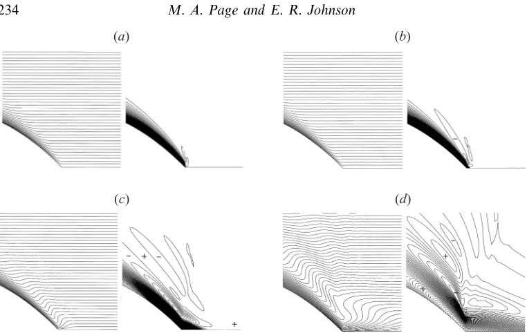
(c) (d)
Figure 6. Numerical solutions of the full equations (2.3) (retaining terms of the form ψxx in
ζ) for flow past the lenticular obstacle (3.3) when α= 64 and L = 8 showing contours of the streamfunctionψ (left) and vorticity ζ (right) in the region of 1
2 6X 6 32 and 06y62. These plots correspond toγ= 0.125 when (a)B=b/γ= 0.125, (b)B= 0.25, (c)B= 0.5, (d)B= 1.0. The contour intervals used are ∆ψ= 0.025 and ∆ζ= 1.
region to merge smoothly with the WBL it is necessary, like in JP93, for there to be an ‘inertial boundary current’ at the outer edge of the WBL, but here this has length
O(γ1/2) inX and a thickness of O(γ3/4) in ˜y. As in JP93, the flow in this inertial layer
is governed by the leading-order conservation of the potential vorticity, Π but here the dominant term in Π isb2ψ
˜
y˜y+h0(1−)(X−1).
Thus fluid that is not expelled from the WBL byX= 1 moves through a sequence of layers near the trailing edge and then rejoins the end of the WBL over a small region within a distance O(γ1/2) ofX= 1. This leads to flow within the WBL similar
to that shown in figure 9 in JP93, but rotated anticlockwise by 90◦. One interpretation
of this is that there is a form of upstream influence extending over the later part of the obstacle, although not able to extend beyond its peak.
Figure 6 shows plots of numerical solutions of the full equations for γ= 0.125 at various values ofB, whenα= 64. These solutions were obtained using the numerical model described in PJ90, which works well in this parameter regime due to the relatively localized nature of the disturbance. The solutions show the broad features outlined above, in particular the general layer structure downstream of the obstacle when B > 1
4. Figure 7 also shows the solution of the full long-obstacle equations
Figure 7.Numerical solutions of the long-obstacle equations (2.8) for flow near the trailing end of the parabolic obstacle (4.2) whenγ= 0.125 andb= 0.03, so thatB= 0.24. This is largest value of
bfor whichΠy remains positive everywhere at this value ofγand it corresponds approximately to
the solution of the full equations in figure 6(b). The contour intervals are as for figure 6.
quantities change sign towards the outer edge of the WBL on the approach to the end of the obstacle, so no solutions of (2.10) are given for that case.
As noted above, the flow upstream of the obstacle remains blocked in this regime, with a ‘stagnant’ region extending over a distance of O(1/γ), and bounded near
y= h(0) by an ‘upstream shear layer’ of scale thickness (Xγ)1/2 which extends over
distances of O(X) upstream. The dynamics of this layer are linear and governed by the same equation (4.9) as the RSL. Near the peak of the obstacle at X = 0 and
y=h(0), there is a ‘shoulder region’, of the same character as that described by Foster (1985) and size of order γ1/3×γ2/3 in terms of γ. This region provides a transition
from the upstream shear layer into the stagnation-point-like character at the start of the WBL.
4.3. Nonlinear flow,γb1
As b/γ becomes large the nonlinear regions described above become increasingly dominated by inertial effects, with the sizes of most of the regions governed by the magnitude of b rather than γ. For example, the WBL has thickness of O(b) once
bγ and its dynamics are governed by the conservation of leading-order potential vorticity Π = b2ψ
˜
y˜y+h(X) along streamlines, with velocities along the layer being of O(1/b). Over the range of bfor which the structure of the layers remains broadly the same as described above, there remains an O(1) flux of fluid into the SBL, which continues to be governed by (4.8), so that its length is of order B =b/γ whenbγ. The dynamics of the flow in the RSL also remains similar to that forb ∼O(γ), so that its thickness is O(b1/2) at the rear of the obstacle. As a result, the final layer
occurrence of γ replaced by band the O(1) lengths replaced by O(b/γ). Despite the fact that the RSL only directly affects the boundary conditions of the WBL over a distance of O(b1/2) from X = 1, there is a significant upstream influence which
extends along much of the length of the WBL through the motion of the fluid in the outer part of that layer which hasu <0 and originates from the RSL. An analysis of the group velocity in the layer reveals that any transient unsteady disturbances travel in the y-direction relative to the fluid motion.
There are, however, significant changes to other parts of the flow, in particular in the upstream shear region which bounds the blocked stagnant region. Within distances of O(1) from the peak of the obstacle, the dynamics of this layer is influenced by inertial effects once bis of O(γ3/4), changing from being governed by the linear heat
equation (4.9) to the full equation (2.8). For larger values of b the same equation remains valid but the thickness of the layer grows from O(γ1/2) in the linear case to
become ofO(b2/3), with the upstream extent of the layer in theX-direction becoming
O(b4/3/γ). Within an O(1) distance of the obstacle, on the approach to the shoulder
region, the layer is governed by the conservation of potential vorticity and it matches directly onto the shoulder region which has size of O(b1/3)×O(b2/3) for bγ. For
distance X of order 1/γ upstream, where the layers near y= ±h(0) merge together, the flow remains governed by the linear heat equation. As a result, the effective length of the ‘stagnant’ blocked region ahead of the obstacle is not significantly affected by the size of b when bγ, although the dynamics of the layer separating it from the uniform flow do change from the linear case.
Further changes to the structure can be expected once b is of order γ1/2, based
on the results in the following section. This regime provides a transition between the structure described above and the form of the flow for b 1 and γ = 0, to be outlined in §5. It can be anticipated that the sizes of the layers which persist for
bγ1/2 will be independent ofγ so that it is unlikely that the SBL/RSL will exist
in this regime, and consequently that the WBL will shed all of its fluid before the end of the obstacle. Similarly, the merging of the upstream layers near y = ±h(0) will be achieved through the conservation of potential vorticity in this regime, rather than through Ekman suction effects over the O(1/γ) lengthscale. The most striking feature, however, will be that the flow will approach a periodic state in y, so that the disturbance is no longer confined to the immediate vicinity of the obstacle.
5. Almost inviscid flow,γmax (1, b2)
5.1. Inviscid flow,γ= 0
For small values ofγ when bis O(1) Ekman pumping is weak and the leading-order flow for X=O(1) is effectively inviscid. Neglecting theγψyyterm from the governing equation (2.8) in the limit as γ→0 leads to a conservation relation for the potential vorticity
Π =b2ψ
yy+y (5.1)
and, assuming that the flow far upstream remains uniform, implies that (see PJ91, for example)
b2ψ
(a) (b)
Figure 8. Plots of the streamfunction ψ (top) and vorticity ζ (bottom) based on the numerical
solution of (5.4) for flow past the parabolic obstacle (4.2) whenγ= 0 and (a)b= 2, (b)b= 1. The solution is plotted over the range 06y610 and the contour intervals used are ∆ψ= 0.25 and ∆ζ= 0.05/b2.
boundary conditions on solutions of (5.2) are that
ψ(X, h(X)) = 0 and ψ(X, y)∼ −y asy→ ∞. (5.3) Lilly & Klemp (1979) discuss precisely this system in the context of two-dimensional linearly-stratified non-rotating hydrostatic flow over long ridges. They note that solutions satisfying (5.2) and (5.3) can be written as
ψ(X, y) =−y+h(X) cos{[y−h(X)]/b}+f(X) sin{[y−h(X)]/b}, (5.4) where f(X) is determined by requiring that energy only radiates upwards at largey. The radiation condition for the β-plane problem here is equivalent to that used for the stratified flow and sof(X) is determined by the same integral equation as derived by Lilly & Klemp, namely
f(X) = 1
π
Z ∞
−∞
h(X0) cos{[h(X0)−h(X)]/b} −f(X0) sin{[h(X0)−h(X)]/b}
X0−X dX0.
They solve this equation numerically using an iterative procedure based on an initial guess for f(X). Durran (1992) introduced an alternative, and simpler, method of obtaining a numerical approximation to f(X) using fast Fourier transforms and his method forms the basis for that used here.
Solution (5.4) and figure 8 show the flow pattern when γ = 0 to be periodic in
y with period 2πb, and to decay over an O(1) distance from both the upstream and downstream ends of the obstacle. In the absence of dissipation the standing waves generated as the flow moves over the obstacle have constant amplitude as y
increases and the ‘shape’ of the obstacle is reflected in the paths of the streamlines at integral multiples of ∆ψ = 2πb. For largebthe velocity componenturemains positive everywhere as in figure 5(a) where γ= 0 and b= 2. Asb decreases a critical value,
a streamline becoming ‘vertical’ and periodicity iny means that vertical streamlines occur for this value ofxat y values 2πb apart. As in the computations of Rottman, Broutman & Grimshaw (1996) for the analogous stratified flow in a finite-width domain, the vertical streamlines occur above the rear of the obstacle. For smaller b
streamlines overturn and it appears that as bpasses through a second critical value,
b2 (say), the first closed streamlines appear. Figure 5(b) with γ= 0 andb= 1 shows
an overturning flow with bc> b > b2. Miles & Huppert (1968) point out that in the
analogous stratified problem it is asbdecreases throughbcthat static stability is first violated. No stability results are available for the present flow. In particular, Arnol’d’s finite-amplitude stability theorems (Arnol’d 1966; McIntyre & Shepherd 1987) give no information. From (5.2),
∂Π
∂ψ =−1, (5.5)
and Arnol’d’s second theorem would apply. This however requires a positive lower bound on the eigenvalues of the negative Laplacian on the flow domain. Since the domain here is unbounded in both x and y the lower bound is zero. When the flow is slightly dissipative stable steady solutions exist with overturning when b < bc as shown by the solution of the full unsteady equations in figure 6(d).
5.2. Weakly damped flow, γ1
With even a small amount of damping present, proportional to γ1 in (2.8), it can be expected that the flow for large values ofywill be irrotational and hence uniform. To account for this limit, a scaled variableY =δyis introduced here, whereδ1 is an undetermined parameter (determined below) which identifies the length scale over which frictional effects act. The introduction of the second vertical variable Y here follows the usual practice for ‘two-variable expansions’ of functions which vary on two widely different length or time scales (see, for example, Kevorkian & Cole 1981). The leading-order solution forγ1 is identical in form to theγ= 0 solution (5.4), so that
ψ=−y+ ReA(X, Y)eiy/b +. . . , (5.6)
but it includes an additional ‘slow’Y dependence of the complex-valued amplitude
A(X, Y) = [H(X, Y)−iF(X, Y)]e−ih(X)/b, (5.7) where H(X, Y) and F(X, Y) are real-valued functions with H(X,0) = h(X) and
F(X,0) =f(X), so that the leading term in (5.6) reduces to (5.4) asY →0 for fixed values ofy. To obtain a higher-order correction forψ, (5.6) can be substituted into
∂(ψ , Π)
∂(X, y) +γψyy= 0, which effectively introduces the higher-order forcing term
γψyy=−bγ2ReAeiy/b +O(δγ/b)
into the linearized equation for the higher-order correction toΠ. It follows that there will be a ‘resonant’ inhomogeneous term in that equation, proportional to eiy/b, unless this forcing is balanced by the additional term
2δbReiAXYeiy/b
terms have the same magnitude provided that δ = γ/b3 and they balance exactly
when Asatisfies the differential equation
2iAXY −A= 0.
There will, of course, be further O(δb) corrections to both Π and ψ, but they will remain of that order for large values of y.
Using a Fourier transform solution for A(X, Y) over k>0,
A(X, Y) = 1 2π
Z ∞
0
ˆ
A(k, Y)eikXdk, (5.8)
as is appropriate for waves which radiate energy upwards (Durran 1992), it follows that ˆA(k, Y) satisfies 2kAˆY + ˆA= 0 and hence that ˆA(k, Y) = ˆA(k,0) exp (−Y /2k) for
k >0, so that
A(X, Y) = 1 2π
Z ∞
0
ˆ
A(k,0)e−Y /2k+ikXdk. (5.9)
The solution for A(X,0), and hence for A(X, Y) through (5.9), is determined by the requirements that it both be consistent with the form
A(X,0) = [h(X)−if(X)]e−ih(X)/b, (5.10) for a given function h(X), and that it also has ˆA(k,0) = 0 fork <0, as in (5.8).
The basis for the iterative method used in this paper is to guess the form of f(X) everywhere, evaluateA(X,0) using (5.10), determine the corresponding approximation to ˆA(k,0) using
ˆ
A(k,0) = Z ∞
−∞A(X,0)e
−ikXdX, (5.11)
then invert the transform (discarding thek <0 components) using (5.8) to yield a new approximation to A(X,0). The corresponding functionf(X) is then obtained from
f(X) =F(X,0) =−ImA(X,0)eih(X)/b ,
based on (5.10) and the process is repeated until it converges. This iteration has been performed numerically remaining in the complex plane and giving a method with some advantages over that used by Durran (1992), in particular convergence at smallerb. Once the iteration converges the functionA(X,0) satisfies both requirements noted above, thereby ensuring that it satisfies the boundary condition on y= 0 and that the solution contains no waves which radiate downwards from y=∞.
Although (5.9) has been derived here under the assumptions that γ is small andb
is O(1), the solution above is valid at any values of γ and b for which δb= γ/b2 is
small, including both the case of rapid flow, where γ is of order one and b1, and the case of blocked flow when γb1. Streamfunction and vorticity plots based on the solutions (5.9) are shown in figure 9 for γ = 0.5 and b= 1, and γ = 1 and
(a) (b)
Figure 9. Plots of the streamfunction ψ (left) and vorticity ζ (right) based on the asymptotic
solution (5.9) for flow past the parabolic obstacle (4.2) when (a)γ= 0.5 and b= 1, (b) γ= 1 and
b= 2. The solution is plotted over the range 06y620 and the contour intervals used are the same as in figure 8.
have a similar character to the corresponding plots forγ= 0, apart from the gradual damping iny, although it is interesting to note that the extrema of both the vorticity and the velocity occur closer toX= 1 asyincreases.
5.3. Long-wavelength flow, b1
In the particular instance of b 1, a further simplification of (5.9) is possible because the e−ih(X)/b term in (5.10) can be neglected to leading order and hence
A(X,0) = h(X)−if(X) in that limit. Using properties of the transforms ˆh(k) and ˆ
f(k), as defined in (5.11), it follows that ˆA(k,0) = 2ˆh(k) for k >0 and therefore (5.9) reduces to
A(X, Y) = 1
π
Z ∞
0
ˆ
h(k)e−Y /2k+ikXdk, (5.12)
provided thatγb2. As for theγ1 case above, the neglected terms in the resulting
expressions for Π andψ are of orderδb relative to the leading-order solution. One potential difficulty with solution (5.9), both in the general case and for b1 in (5.12), is in resolving its behaviour near the essential singularity in the transform
ˆ
A(k, Y) at k = 0 due to the exp (−Y /2k) term. The effects of this singularity can be investigated further by examining the solution (5.12) for the special case when
ˆ
h0(k) =πexp (−|k|), which corresponds to the obstacle
h0(X) = 1 +1X2, (5.13)
because an exact solution for A(X, Y) is available in this case (see, for example, Gradshteyn & Rhyzik 1965, equation 3.324.1), given by
A0(X, Y) =
2Y
1−iX
1/2
K1([2Y(1−iX)]1/2) (5.14)
whereK1 is the modified Bessel function of the second kind of order one.
Asymptot-ically, this solution has the form
A0(X, Y)∼ π
1/2Y1/4
21/4(1−iX)3/4e−[2Y(1−iX)]
1/2
for |Y(1−iX)| 1,
Figure 10.Plots of the streamfunctionψ(left) and vorticityζ(right) based on the exact solution (5.14) forb 1 flow past a ‘Witch of Agnesi’ obstacle when γ = 1 and b = 2, illustrating the damping effect present forγ >0. The solution is plotted over the range 06y620 and the contour intervals used are the same as in figure 8.
for frictionless flow in that case. The solution (5.14) is plotted in figure 10 forb= 2 which, although it is not large, illustrates the damping effect that the Ekman pumping has on the stationary wavefield over the obstacle, with an exponential decay of the vorticity in both theX- andy-directions. No streamlines overturn in this limit (even for γ= 0 when b1) but there is an O(1) reduction in the maximum of u(caused by fluid rising over the obstacle) for the entire parameter range over which (5.14) remains valid, including when γ is very large (provided it is less than O(b2)). Note
also that the smoothness of the obstacle shape in this case avoids the problems with discontinuities in ˜v, for example, but it does not affect any other major features of the flow.
The exact integral (5.14) can also be used to help obtain the numerical solution for other functions h(X) because, by subtracting the appropriate multiple of 1/(1−iX) from A(X,0) to ensure that the transform of the remainder is zero at k = 0, it is possible to evaluate (5.9) numerically without encountering some of the difficulties in resolution neark = 0 which would otherwise result from the exp (−Y /2k) term in the transform. As (5.14) is exact, this is not only possible for b1 but can be used in any case for which (5.9) is appropriate.
6. Conclusion
This paper has considered the steady flow patterns forced on aβ-plane by obstacles long in the zonal direction. The restriction to long obstacles reduces the number of parameters in the oceanographic limit of vanishingly small Ekman and Rossby numbers to two: γ, giving the length of the obstacle in terms of the Ekman decay scale, andb, a Rossby-wave Froude number.
A novel numerical technique has allowed the (γ, b)-space to be explored econom-ically and the bounded region of parameter space where flows overturn has been identified for a parabolic obstacle. Asymptotic solutions have been given for blocked flow (b1), including linear flow (bγ1), weakly nonlinear flow (b∼γ 1) and nonlinear flow (γ b 1), identifying the various thin boundary layers that appear. Solutions have also been given for almost-inviscid flow,γmax (1, b2) where
the disturbance is weakly damped and decays away abreast of an obstacle over a length scale of order b3/γ.
equations, where it has the advantage that the propagation of information upstream by Rossby waves, through the integration forψalong lines of constantΠ, is accomplished within each timestep. This is essential for the accurate modelling of these flows because the long Rossby waves, which havek andl small in (2.9), travel rapidly upstream.
The leading-order viscous effect in the flows considered here is the destruction of vorticity throughout the flow field by Ekman pumping. In the present limit horizontal viscous effects are confined to layers of thicknessE1/4, thinner that the mass-carrying
WBL and its extensions provided tanβ E1/4. If the E1/4 layers remain attached
they do not affect the flow. If the boundary layers become sufficiently nonlinear the
E1/4 layers can separate from bluff bodies. This is discussed in greater detail in JP93
and PJ90 where it is noted that separation bubbles in eastward flow are small and appear likely to have little effect on flow past obstacles with tapering leeward profiles. The region of parameter space least explored is the interior of the overturning regime. The asymptotic analysis of §§4.2, 4.3 remains valid just inside this region and gives a description of the boundary-layer structure and return flows possible. Numerical solutions of the full equations without the long-wave approximation show, as in figure 6(d), that stable steady solutions are possible. However it seems likely that steady solutions may not exist or may be unstable for many points within the overturning region. From computations for the analogous stratified two-dimensional non-rotating flow Rottman et al. (1996) conclude that internal waves trapped in the neighbourhood of an obstacle can lead to an inherently unsteady flow and an almost-periodic oscillation in the drag on the obstacle. This would imply here that Rossby waves trapped near the obstacle prevent the flow from settling to a steady state. There are however differences between the present flow and those of Rottman et al. (1996) and Grimshaw & Yi (1990, 1993). Their flows are effectively inviscid, lacking an equivalent of vorticity destruction by Ekman pumping. Further, their flows have Froude numbers of order the channel width and so are strongly affected by horizontal upper boundaries reflecting vertically-propagating long waves back into the flow domain. The exploration of the overturning region remains a challenging problem that will be addressed elsewhere.
It was noted in§5 that for even stronger forcing of the lee waves over the obstacle it is possible for closed streamlines to form in the Long’s model solution for the short-obstacle flow (see, for example, Miles & Huppert 1968) and that they also appear to form for the long-obstacle γ= 0 flow below a small enough value ofb, b2. They may
also be expected to form for small values ofγ. The numerical method described here is however no longer suitable asuvanishes at many points in such flows. The iterative method described in §5 for calculating the γ = 0 solution also fails at values of b
below about 0.5 for the parabolic obstacle. Whether closed streamlines are possible in stable steady flow solutions to the full equations forbmoderately small but B =b/γ
large has not been determined yet. The comments in PJ90 relating to the resonant case shown in figure 15 there further support the argument that although such closed-streamline solutions can exist, they may not be stable and that a stable flow could also exist at the same values of band γbut with different upstream conditions.
Appendix. Blocked flow past a triangular obstacle
Consider equation (2.8) with b= 0 for the triangular obstacle
h(X) =
1− |X| for |X|61