Monash University, Wellington Road CLAYTON Vic 3800 AUSTRALIA
Telephone: from overseas:
(03) 9905 2398, (03) 9905 5112 61 3 9905 2398 or 61 3 9905 5112
Fax:
(03) 9905 2426 61 3 9905 2426
e-mail: impact@buseco.monash.edu.au
Internet home page: http//www.monash.edu.au/policy/
How would global trade liberalization affect
rural and regional incomes in Australia?
by
K
YM
ANDERSON
University of Adelaide and
World Bank
J
AMES
GIESECKE
Centre of Policy Studies
Monash University
AND
E
RNESTO
VALENZUELA
University of Adelaide
General Paper No. G-176 July 2008
ISSN 1 031 9034 ISBN 0 7326 1583 6
i
How would global trade liberalization affect
rural and regional incomes in Australia?
Kym Anderson
(University of Adelaide and World Bank)
kym.anderson@adelaide.edu.au
James Giesecke
(Monash University)
James.Giesecke@buseco.monash.edu.au
Ernesto Valenzuela
(University of Adelaide)
ernesto.valenzuela@adelaide.edu.au
July 2008
iii
I Introduction 1
II Distortions to Agricultural Incentives Since the 1950s 2
III Modelling Approach 8
(i) The Global (Linkage) Model 8
(ii) The Australian (TERM) Model 9
(iii) Simulation Design 10
(iv) Model Closure 13
IV Results: Effects of Distortions on Incomes of Australian Farmers
and Rural Areas 14
V The Bottom Line 16
REFERENCES 17
APPENDIX Derivation of export demand elasticities implicit in
LINKAGE’s parameters and theoretical structure 29
Table 1 Impact of rest of world’s trade policies on prices and volume of
Australia’s exports and imports, 2004 20
Table 2 National macroeconomic results, Australia, 2004 21
Table 3 Aggregate sectoral real income effects, Australia, 2004 22
Figure 1 Nominal rates of assistance to manufacturing, all non-agricultural tradables, all agricultural tradable industries, and relative rate
of assistance,a Australia, 1946-47 to 2004-05 23
Figure 2 Relative rates of assistance to agriculture,a Australia and other
high-income countries, 1955 to 2004 24
Figure 3 Relative rates of assistance to agriculture,a high-incomeb and
developing countries, 1955 to 2004 25
Figure 4 Changes in sectoral output, Australia, 2004 26
Figure 5 Regional income impacts in Australia, 2004 27
Figure 6 Geographical distribution of real gross regional product outcomes
iv
Appendix Table 2 Sectoral shares of gross regional product and regional
shares of GDP and population, Australia, 2004 33
Appendix Table 3 Commodity-specific import price shocks, and estimates
of export price impacts on Australia, 2004 35
Appendix Figure 1 The LINKAGE Model’s commodity sourcing structure 36
Appendix Figure 2 Transmitting export results from the global to the
rural and regional incomes in Australia?
For decades rural Australia has been discriminated against by industrial policies at home and agricultural protectionism abroad. While agricultural export taxation in poor countries had the opposite impact, recent reforms there mean that that offsetting effect on Australia has diminished. There has also been some re-instrumentation of rich-country farm policies away from trade measures. This paper draws on new evidence to examine whether Australian farmers and rural regions are still adversely affected by farm price-distortive policies abroad, using a global and a national economy-wide model. The results vindicate the continuing push by Australia’s rural communities for multilateral agricultural trade liberalization.
I Introduction
Throughout the post-World War II period Australian farmers have been
discriminated against by policies at home and abroad. At home, Australia’s
manufacturing protection policies far more than offset the country’s agricultural support
policies, so the farm sector and farm household incomes were smaller than they would
have been without those policies. But domestic reforms in the past three decades have
virtually removed that part of the discrimination. Abroad, the Australian farm sector was
an indirect beneficiary, through improved terms of trade, of anti-agricultural policies of
developing countries such as export taxes, but has been harmed by pro-agricultural
policies in other high-income countries. While the former have greatly diminished over
the past quarter-century, the latter are still rife even though their nature and sources have
altered somewhat recently.
This paper seeks first to summarize new research results showing the changing
world, drawing on the results of a new World Bank multi-country research project, and
second to provide economy-wide modeling results of the impact of remaining distortions
on farm versus non-farm incomes and on rural versus other areas in Australia.
The Australian case is different from that of other high-income countries in at
least two respects. First, agriculture has never been assisted more than non-agricultural
sectors in Australia, in contrast to virtually all other OECD countries. In that sense it is
much more like an agricultural-exporting developing country. And second, since the
mid-1970s Australian exports of minerals and energy raw materials have dominated its
exports of farm products. Hence agricultural protectionism abroad hurts Australian
farmers and rural areas not only relative to urban areas but also relative to (mainly
remote) areas specializing in mining.
The paper is organized as follows. After summarizing results from the World
Bank’s agricultural price distortion project for Australia and for the rest of the world over
the past half-century, we describe the two-stage modeling approach used. The first stage
involves modeling the net impact on Australia’s terms of trade of distortions to
agricultural and other goods markets abroad as of 2004 (derived from the World Bank’s
Linkage CGE model of the global economy); the second modeling stage uses the TERM
CGE multi-regional model of the Australian economy to estimate the regional and net
farm vs nonfarm income consequences of the terms of trade effects of those
discriminatory policies as of 2004. We then discuss model results, before drawing out
some implications of alternative future policies for Australia’s rural areas. We point out
that while the growth of agricultural protection in rich countries has reversed a little
farmers to slightly assisting them relative to their manufacturers. If this trend continues,
Australian farmers and rural regions will have even more reason to press for an ambitious
reform outcome from the agricultural part of the multilateral trade negotiations under the
WTO’s Doha Round.
II Distortions to Agricultural Incentives Since the 1950s
Australia’s Industries Assistance Commission began calculating estimates of the
nominal rates of assistance (NRA, the percentage by which government policies have
raised gross returns to producers above what they would be without the government’s
intervention) for major agricultural commodities beginning with the year 1970-71. This
series has been continued by its successors, the Industry Commission and the
Productivity Commission. For the years before 1970-71, a comprehensive series is
published in Lloyd (1973, pp. 149-58). It covers the major agricultural commodities for
which data were available at the time, for the years 1946-47 to 1970-71.
The Lloyd and Commission series use essentially the same methods.
Commodities are designated as either export or import-competing and then direct
estimates of the implicit price changes to producers resulting from agricultural assistance
are made and expressed as a percentage of the export or (in the case of tobacco and cotton
pre-1970) the import parity price. Anderson, Lloyd and MacLaren (2007) bring these
series together and obtain the weighted averages for agriculture as a whole by assuming
the NRA was zero for products not covered by the above estimates. As weights they used
domestic producer prices by (1+NRA/100). Their results, which include
‘non-product-specific’ assistance such as via factor and intermediate input markets, show that the
average nominal rate of agricultural assistance rose during the 1950s and 1960s but
subsequently declined so that by the end of the 1990s its average was virtually zero
(middle line in Figure 1). So too did the dispersion of industry NRAs within the farm
sector: the standard deviation around the weighted mean peaked at more than 50 percent
in the early 1970s, but is now less than 0.5 percent (Anderson, Lloyd and MacLaren
2007).
It is relative prices and hence relative rates of government assistance that affect producers’ incentives, not just agricultural prices alone. In a two-sector model an import
tax has the same effect on the export sector as an export tax (the Lerner (1936) Symmetry
Theorem), and this carries over to a model that also includes a third sector producing only
non-tradables (Vousden 1990, pp. 46-47). It was this understanding that led Gruen (1968)
to point out that raising assistance to agriculture in the presence of high assistance to
manufacturing could increase rather than reduce national economic welfare. For that
reason it is necessary to report estimates not only of the average nominal rate of
assistance (NRA) for the tradable parts of the agricultural sector, but also of the average
NRA for the tradable parts of all non-agricultural sectors, based on NRA estimates for
individual industries. With those two sectoral NRAs we can then calculate a Relative
Rate of Assistance, RRA, defined as:
RRA = 100[(1+NRAagt/100)/(1+NRAnonagt/100) – 1] (1)
where NRAagt and NRAnonagt are the average percentage NRAs for the tradables parts
less than -100 percent if producers are to earn anything, so too must the RRA. This
measure is useful: if it is below zero, it provides an internationally comparable indication
of the extent to which the policy regime has an anti-agricultural bias, and conversely
when the RRA is positive.
Estimates of the NRA for manufacturing for the period prior to 1968-69, when
Tariff Board estimates begin, rely on tariffs only. During 1952 to 1960 there were also
protective quantitative restrictions on imports of manufactures, but since estimates of the
protective effects of those import licenses are unavailable, Anderson, Lloyd and
MacLaren (2007) assume their impact on the average NRA for non-agricultural tradables
is exactly offset by the negative impact of the ban on key mining exports in those years.1
Since Australia’s imports pre-1969 were almost exclusively manufactures, customs
revenue as a percentage of the value of all merchandise imports provides a reasonable
proxy for the country’s nominal rate of tariff protection for manufacturing. For the period
since 1968-69, the Productivity Commission and its predecessors provide estimates of
both nominal and effective rates of assistance to manufacturing, for industry
sub-categories down to the 4-digit level.In addition to tariffs these cover subsidies, bounties,
discriminatory sales taxes and, from 1982-83, quantitative restrictions and local content
plans.
The weighted average nominal rate of assistance on outputs (NRAs) for the whole
non-agricultural tradables sector is generated by assuming only (and all) service sectors
1 In years prior to the 1950s, the relatively low international prices of mineral and energy products (World
produce non-tradables, and that non-agricultural primary sectors received a zero NRA on
average. It is shown as the upper line in Figure 1, with the manufacturing-only NRA
shown just below it (indicating that the weight of non-farm primary activities is very
low). Once NRAs are available for both farm and non-farm tradable sectors, it is a simple
matter to calculate the RRA, using the formula in equation (1) above. That is shown as
the lowest of the lines in Figure 1.
These estimates reveal two key facts. First, for all of the post World War II period
Australian sectoral and trade policies have discriminated against the agricultural sector
(and even more so the mining sector). Even though production subsidies were given to
farmers for most years from the early 1950s to the late 1990s, the assistance they received
was much less than that provided to manufacturing via import barriers. Hence the relative
rate of assistance (RRA) has been negative. Second, it is clear from Figure 1 that the
extent of Australian policy discrimination against farmers has more or less continuously
declined throughout that period and has now almost disappeared. The only manufacturing
protection remaining is for textiles and motor vehicles, and even those tariffs are
scheduled for further cuts in 2010.
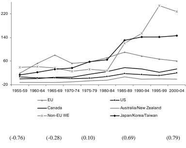
Australia contrasts with other high-income countries. According to new results
from a World Bank research project that provides results for more than 70 countries
accounting for 90 percent of global agriculture (Anderson 2009a), all have followed a
similar path to Australia’s in the sense of raising their relative rates of assistance to
farmers as their national incomes have risen. However, except for New Zealand, those
RRAs have risen from higher bases and to higher levels than Australia, and more so the
hint of a structural break to the growth of agricultural protection around the time of the
Uruguay Round Agreement on Agriculture coming into force in 1995, no other OECD
country except New Zealand has made as dramatic a reduction in agricultural assistance –
in terms of driving the RRA towards zero – as Australia.
Developing countries, on the other hand, are on average much more like
Australia, although their RRAs were even lower in the early years of their independence
from imperial powers, and some have risen even faster than Australia’s. Indeed as a
group they have now ‘overshot’, in the sense that their average RRA is above zero for
developing countries as a whole (Figure 3). In the past, those disincentives to developing
country farmers assisted Australia and other agricultural-exporting countries by making
farm products scarcer in international markets. By the turn of the century, however, their
policies were adding to the downward pressure on prices in international food markets
caused by high-income country policies.
That is, taken together these estimated RRAs suggest that by 2004 the policies of
both high-income and developing countries were depressing the international prices of
farm products. Their weighted average moved from being negative to being positive in
the 1980s.2 These facts suggest that the prices received by farmers in an open,
non-distorting country such as Australia were depressed in 2004 by policies in the rest of the
world. But to determine by how much, the new price distortion estimates need to be
inserted in a model of the world’s trading nations that is capable of generating their
2 That timing is consistent with the modelling finding by Tyers and Anderson (1992, Table 6.9) that as of
impact on Australia’s terms of trade, which in turn need to be inserted in a model of the
Australian economy that is disaggregated sectorally and regionally.
III Modelling Approach
The above suggests that to get a sense of just how much agricultural and trade
policies abroad are impacting on farmers and others in Australia, a two-stage modeling
procedure is needed. For the first stage we use a global model to estimate the net impact
on Australia’s terms of trade of distortions to agricultural and other goods markets abroad
in 2004 (known as the Linkage Model, described in van der Mensbrugghe 2005). For the
second stage, a national model with regional details (known as the TERM Model,
described in Horridge, Madden and Wittwer 2005) is used to estimate the regional
consequences of the terms of trade effects of those discriminatory policies. Since
Australia had virtually no sectoral or trade distortions of its own by 2004, there is no need
to also simulate own-country reform.
(i) The Global (Linkage) Model
Global results, based on the comparative static version of the LINKAGE model, use
a modified version of the latest release of the GTAP database, in that the distortions to
developing country agriculture are replaced with ones from the World Bank’s new
estimates of distortions to agricultural incentives (from Anderson and Valenzuela 2008).
These simulated global results are transmitted to the Australian national model via
as vertical shifts in the export demand curves (that is, of the willingness to pay for
Australian exports – see below).
(ii) The Australian (TERM) Model
The national results use the Australian TERM model, which is a "bottom-up"
CGE model with features that enable it to deal with the detailed behavior of producers,
consumers and government economic agents in many regions of the country. We simulate
the impacts of the removal of current distortions to world markets on Australia by
dividing the national economy into 59 regions (Statistical Divisions) and 27 industrial
sectors. We also define three super-regions of urban, rural and mining localities, based on
the ratio of the sectoral value added share for each region to the national share of sectoral
value added (see Appendix Tables 1 and 2 for the regional and sectoral classifications
and the regions’ relative sectoral value added shares, respectively). The 13 urban regions
comprise just over 73 percent of the population and 71 percent of national GDP, and the
13 mining regions comprise 9 percent of the nation’s population and 13 percent of GDP.
Thus the 33 rural regions account for the residual 18 percent of the population and 16
percent of GDP.
The data structure in TERM allows the model to capture explicitly the behavior of
industries, households, investors, exporters and the government all at the regional level.
The model’s theoretical structure is based on that of the well-known CGE model, ORANI
(Dixon et al. 1982). Producers in each regional industry are assumed to maximize profits
subject to a production technology that allows substitution between primary factors
inputs. A representative household in each region purchases goods in order to obtain the
optimal bundle in accordance with its preferences and its disposable income. Investors
seek to maximize their rate of return. In the short-run, this desire is expressed as a
positive relationship between regional industry investment and rates of return. In the
medium- to long-run assumed here, it is expressed as the endogenous physical capital
supply to each regional industry at exogenous rates of return.
Commodity demands by foreigners are modeled via export demand functions that
capture the responsiveness of foreigners to changes in Australian supply prices.
Economic agents decide on the geographical source of their purchases according to
relative prices and a nested structure of substitution possibilities. The first choice facing
the purchaser of a unit of a particular commodity is whether to buy one that has been
imported from overseas or one that has been produced in Australia. If an Australian
product is purchased, a second decision is made as to the particular region the commodity
originates from. It is assumed that Australian-made brands are considerably more
substitutable than is an Australian brand with a foreign brand. The national data include
regional margins for transportation and retailing, with the possibility of substitution of the
margins sources based on their relative prices.
(iii) Simulation Design
Anderson, Valenzuela and van der Mensbrugghe (2009), for a wide range of
countries, present terms of trade results from the World Bank’s LINKAGE model under a
long-run scenario in which world agricultural and other goods market distortions are
paper we use the TERM model to assess the implications of that set of price impacts at
Australia’s national border for various sectors and regions of its economy. To do so, we
must translate into TERM inputs or shocks the two sets of LINKAGE outputs:
movements in foreign currency prices for Australian imports, and vertical (willingness to
pay) movements in foreign demand schedules for Australian exports.
For movements in foreign currency import prices, the communication of results
between the two models is relatively straightforward. We translate movements in foreign
currency import prices classified by LINKAGE commodity into movements in foreign
currency import prices classified by TERM commodity via equation (1).
Hc,k(M) ( ,2)(cTermr)* Hc,t(M) ( ,2)(tLinkage)*
k Linkage t Linkage
p p
∈ ∈
⎡ ⎤
=
⎢ ⎥
⎣
∑
⎦∑
(c∈COM,r∈REG) (1)where H(M)c,k is a matrix of values showing the distribution of imports of TERM
commodity c across LINKAGE commodities k; ( ,2)( )*
Term c r
p is the percentage change in the
foreign currency price of TERM commodity c used in region r; and ( )* ,2
Linkage t
p is the
percentage change in the foreign currency price of TERM commodity t (values for which
are reported in column 3 of Table 1). Results for (,2 )*
Term c
p are reported in column 2 of
Appendix Table 3. Notice that in equation (1) the exogenous percentage movements in
the foreign currency price of commodity c ( ( )* ( ,2)
Term c r
p ) are assumed to be identical across all
regions, a feature of our shocks that assists in the interpretation of regional results.
Translating LINKAGE results for foreign currency export prices into TERM
shocks is more complicated. As Horridge and Zhai (2006) argue with the help of
willingness-to-pay shifts implicit in the price and quantity movements produced by the
global model. Horridge and Zhai show that these can be calculated via the formula:
fpt(Linkage) = pt(Linkage)*+qt(Linkage)*/ηt(Linkage) (2)
where fpt(Linkage) is the percentage vertical shift in the export demand schedule for
LINKAGE commodity t; pt(Linkage)* is the percentage change in the foreign currency
export price for LINKAGE commodity t; qt(Linkage)* is the percentage change in the
quantity of exports of LINKAGE commodity t; and ηt(Linkage) is the export demand
elasticity for LINKAGE commodity t. Unlike national models, where the export demand elasticity typically appears as an explicit parameter, in global models like LINKAGE and
GTAP, ηt(Linkage) is implicit in the theory and parameters governing how agents in each
country substitute between alternative sources of supply for each commodity. We explain
our method for calculating ηt(Linkage) in the Appendix. Column (4) of Table 1 reports our
(Linkage)
t
η estimates.
The results for fpt(Linkage) are translated to vertical shifts for TERM commodities,
(4)
c
f , via equation (3).
(X) (4) (X) ( )
c,k , c,t
H c r H tLinkage k Linkage t Linkage
f fp
∈ ∈
⎡ ⎤
=
⎢ ⎥
⎣
∑
⎦∑
(c∈COM,r∈REG) (3)where H(X)c,k is a matrix of values showing the distribution of the value of TERM exports
of commodity c across LINKAGE commodities k; (4) ,
c r
f is the vertical shift in the TERM
export demand schedule for commodity c from region r; and fpt(Linkage) is the vertical shift
reported in the first two columns of Table 1. Results are reported in column 1 of
Appendix Table 3. Like equation (1), equation (3) assumes that the movements in
commodity-specific export demand schedules ( fc r(4), ) are identical across regions. This
will prove useful in interpreting the regional results below.
(iv) Model Closure
We use a long-run comparative-static closure of TERM. This closure has the
following characteristics:
• Physical capital is in elastic supply to each regional industry at exogenous rates of
return;
• Agricultural land supplies are exogenous and land rental rates are endogenous;
• National employment is exogenous and the national real wage is endogenous;
• National population is exogenous and, subject to this constraint, regional
populations follow regional employment outcomes;
• Labour is largely free to move between regions, although there is some regional
stickiness in labour supply by allowing the gap between the regional wage and the
national wage to be positively related to the movement in regional employment;
• Regional industry investment/capital ratios are exogenous and national investment
is endogenously determined as the sum of regional industry investments;
• National consumption (public plus private) is a fixed proportion of gross national
disposable income and, subject to this national constraint, private consumption at
• The ratio of real public consumption spending to real private consumption
spending in each region is exogenous.
IV Results: Effects of Distortions on Incomes of Australian Farmers and Rural Areas
To understand the impacts through the terms of trade effects on Australia of the
rest of the world’s farm and trade policies, we begin with the macroeconomic effects
before turning to the sectoral and regional results. The macro impacts are decomposed
into two effects: those attributable to changes in demand for Australian exports (column 1
of Table 2); and, those attributable to changes in the prices Australia pays for its imports
(column 2). Column 3 reports the sum of those two effects.
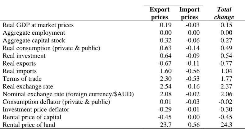
Removal of distortions in global goods markets has a favourable effect on
Australia’s terms of trade: they improve by 1.8 percent, made up of a 2.3 percent
improvement in export prices and offset by a 0.5 percent change in import prices (Table
2, row 8). The increasing demand for agricultural exports lifts rental rates on agricultural
land, by almost one-quarter (24 percent, row 14). Together with the increase in the terms
of trade, this encourages expansion of the long run national capital stock (row 3). With
the capital stock higher than otherwise, so too is real GDP (row 1). The positive
movements in real GDP and the terms of trade account for the positive outcome for real
consumption (row 4), which rises by 0.5 per cent relative to what it would otherwise have
been. Approximately 0.35 percentage points of the total outcome for real consumption is
attributable to the positive terms of trade outcome, with the remaining 0.15 percentage
trade allows the real GNE outcome to exceed the real GDP outcome. This accounts for
the movement towards deficit in the real balance of trade, which is expressed as a
contraction in the aggregate volume of exports and an expansion in aggregate import
volume (rows 6 and 7, column 3). The mechanism that achieves this is real appreciation,
amounting to 2.4 percent (row 9 of Table 2).
That real appreciation of the exchange rate means tradable sectors whose prices
do not rise much could be under pressure to contract. And indeed this is what happens.
The bias towards agriculture in the improvement in Australia’s terms of trade ensures that
output of agricultural and food manufacturing industries expand, but the real exchange
rate appreciation causes other main trade-exposed sectors to contract. This can be seen
from Figure 5, where it is evident that virtually all agricultural and food industries expand
(with dairying and rice benefiting most) but other manufacturing output shrinks by about
1 percent overall, and mining output shrinks by 2 percent.
Our modelling assumes all regions within Australia experience the same
commodity-specific percentage changes in export and import prices from removal of
world agricultural and other trade distortions. As a result, regional differences in the
industrial composition of local economic activity determine much of the dispersion in
regional economic impacts.3 That is, regional income effects are strongly positive for
rural regions, slightly negative for mining-intensive regions (the less-agricultural regions
of Western Australia and South Australia, the Northern Territory, and Mackay and
3 Adams, Horridge and Parmenter (2000) show that an industry can make a positive contribution to a
region’s relative growth rate if it is a fast (slow)-growing industry and is over (under)-represented in the region, or if it grows more quickly in the region than it does in the nation as a whole. In applying the LINKAGE model results to the bottom-up regional model TERM, we had no basis for differentiating the region-specific shocks to commodity-specific import and export prices. Hence, with the sizes of
Fitzroy in Queensland), and mixed for urban regions (Figure 6). The urban results depend
among other things on the extent to which an urban centre is specialized in servicing
more the agricultural sector (as with Adelaide and Melbourne) rather than the mining
sector (as in Perth and Darwin, which is where many miners live when they are not
working on remote mine sites). In terms of geography, these output results are reported
also on the map of Australia (Figure 7).
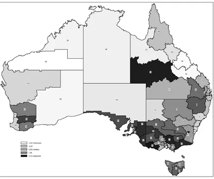
Notice from Figure 6 that the income gains to rural areas are by no means
uniform. Indeed there is a wide variation, ranging from less than 0.1 percent in Far North
Queensland (where mining also occurs – see Appendix Table 2) to more than 4 percent in
the agriculturally lush Western Districts of Victoria. Again this reflects the regional
differences in the industrial composition of local economic activity, given the wide range
of output changes shown in Figure 5. It also correlates with the regions most adversely
affected by drought recently (see Horridge, Madden and Wittwer 2005) and by
Dutch-disease effects flowing from the mining boom (Horridge and Wittwer 2008).
V The Bottom Line
The key net effects of the changes reported above are that real net rural incomes
in Australia would be 1.2 percent higher, and real returns to agricultural land in particular
would be 24 percent higher, in the absence of price distortions resulting from agricultural
and trade policies in the rest of the world.4 Clearly those policies abroad are hurting
Australia’s rural households, adding to the adverse impact of drought over recent years
4 Even though incomes in mining regions would be 0.7 percent lower on average, those regions currently
(Horridge, Madden and Wittwer 2005, Horridge and Wittwer 2008). The upturn in
international food prices in 2007-08 has brought a welcomed reprieve, and Australian
farmers and trade negotiators are hoping that upturn might help revive the agricultural
part of the multilateral trade negotiations under WTO’s Doha Development Agenda. As
shown in Anderson and Martin (2006), nothing short of a very ambitious reform outcome
from those negotiations is needed to ensure this source of discrimination by agricultural
protectionist countries towards rural communities in agricultural-exporting countries is
permanently reduced.
REFERENCES
Adams, P.D., M.J. Horridge and B.R. Parmenter (2000), “Forecasts for Australian
regions using the MMRF-GREEN model”, Australasian Journal of Regional Studies 6(3): 293-322.
Anderson, K. (ed.) (2009a), Distortions to Agricultural Incentives: A Global Perspective, 1955-2005,London: Palgrave Macmillan and Washington DC: World Bank (forthcoming).
Anderson, K. (ed.) (2009b), Agricultural Price Distortions, Inequality and Poverty, London: Palgrave Macmillan and Washington DC: World Bank (forthcoming).
Anderson, K., R. Lattimore, P.J. Lloyd and D. MacLaren (2009a), “Distortions to
Agricultural Incentives in Australia and New Zealand”, Ch. 6 in Anderson (2009).
Anderson, K., P.J. Lloyd and D. MacLaren (2007), ‘Distortions to Agricultural Incentives
Anderson, K. and W. Martin (eds.) (2006), Agricultural Trade Reform and the Doha Development Agenda, London: Palgrave Macmillan and Washington DC: World Bank.
Anderson, K. and E. Valenzuela (2008), Global Estimates of Distortions to Agricultural Incentives, 1955-2005, spreadsheet available at www.worldbank.org/agdistortions
from October.
Anderson, K., E. Valenzuela and D. van der Mensbrugghe (2009), “Global Effects of
Agricultural and Trade Policies Using the Linkage Model”, Ch. 2 in Anderson
(2009b).
Dixon, P.B., B.R. Parmenter, J. Sutton, and D.P. Vincent (1982), Orani: A Multisectoral Model of the Australian Economy, Amsterdam: North Holland.
Dixon, P.B. and M.T. Rimmer (2002), Dynamic General Equilibrium Modelling for Forecasting and Policy: A Practical Guide and Documentation of MONASH, Contributions to Economic Analysis 256, Amsterdam: North-Holland.
Gardner, B. (2009), “Distortions to Agricultural Incentives in the United States and
Canada”, Ch. 5 in Anderson (2009a).
Gruen, F.H. (1968), “Welfare Economics, the Theory of the Second Best, and Australian
Agricultural Policy”, mimeo, Monash University, Clayton, Vic.
Hayami, Y. and M. Honma (2009), “Distortions to Agricultural Incentives in Japan,
Korea and Taiwan”, Ch. 3 in Anderson (2009a).
Horridge, J.M., J.R. Madden and G. Wittwer (2005), ‘Impact of the 2002-03 Drought on
Horridge, M. and G. Wittwer (2008), “Creating and Managing an Impossibly Large CGE
Database that is Up-to-date”, Paper presented at the 11th Annual Global Economic
Analysis Conference, Helsinki, 12-14 June.
Horridge, J.M. and Zhai, F (2005), “Shocking a Single-Country CGE Model with Export
Prices and Quantities from a Global Model”, annex to Chapter 3 in T.W. Hertel
and L.A. Winter (eds.) Poverty and the WTO: Impacts of the Doha Development Agenda, London: Palgrave Macmillan and Washington DC: World Bank.
Josling, T. (2009), “Distortions to Agricultural Incentives in Western Europe”, Ch. 4 in
Anderson (2009a).
Lerner, A.P. (1936), “The Symmetry Between Import and Export Taxes”, Economica
3(11): 306-13, August.
Lloyd, P.J. (1973), Non-tariff Distortions of Australian Trade, Canberra: Australian National University Press.
Tyers, R. and K. Anderson (1992), Disarray in World Food Markets: A Quantitative Assessment, Cambridge and New York: Cambridge University Press.
van der Mensbrugghe, D. (2005), ‘LINKAGE Technical Reference Document: Version
6.0,’ Unpublished, World Bank, Washington DC, January 2005. Accessable at
www.worldbank.org/prospects/linkagemodel
Vousden, N. (1990), The Economics of Trade Protection, Cambridge and New York: Cambridge University Press.
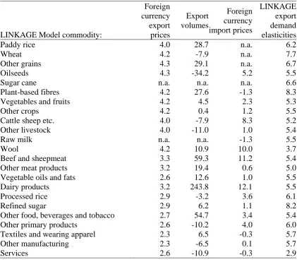
Table 1: Impact of rest of world’s trade policies on prices and volume of
Australia’s exports and imports, 2004
(LINKAGE Model results, long-run percentage change relative to baseline)
LINKAGE Model commodity:
Foreign currency export prices
Export volumes
Foreign currency import prices
LINKAGE export demand elasticities
Paddy rice 4.0 28.7 n.a. 6.2
Wheat 4.2 -7.9 n.a. 7.7
Other grains 4.3 29.1 n.a. 6.7
Oilseeds 4.3 -34.2 5.2 5.5
Sugar cane n.a. n.a. n.a. 6.6
Plant-based fibres 4.2 27.6 -1.3 8.3
Vegetables and fruits 4.2 4.5 2.3 5.3
Other crops 4.2 0.4 1.2 5.5
Cattle sheep etc. 4.0 -7.9 8.3 5.2
Other livestock 4.0 -11.0 1.0 5.4
Raw milk n.a. n.a. -1.3 5.5
Wool 4.2 10.9 10.0 3.7
Beef and sheepmeat 3.3 59.3 11.2 5.4
Other meat products 3.2 19.4 0.6 5.0
Vegetable oils and fats 2.6 12.6 1.0 5.5
Dairy products 3.2 243.8 12.1 5.5
Processed rice 2.9 -3.2 3.6 6.1
Refined sugar 2.9 6.2 1.1 8.2
Other food, beverages and tobacco 2.7 54.7 3.4 5.4
Other primary products 2.6 -10.2 4.0 6.0
Textiles and wearing apparel 2.3 6.5 -0.3 5.7
Other manufacturing 2.3 -6.5 0.1 5.7
Services 2.6 -10.9 -0.3 2.9
Table 2: National macroeconomic results, Australia, 2004
(percent)
Due to changes in:
Total change Export
prices
Import prices
Real GDP at market prices 0.19 -0.03 0.15
Aggregate employment 0.00 0.00 0.00
Aggregate capital stock 0.32 -0.06 0.27
Real consumption (private & public) 0.63 -0.14 0.49
Real investment 0.64 -0.09 0.54
Real exports -0.67 -0.11 -0.77
Real imports 1.60 -0.56 1.04
Terms of trade 2.30 -0.53 1.77
Real exchange rate 2.54 -0.16 2.37
Nominal exchange rate (foreign currency/$AUD) 2.08 -0.02 2.06
Consumption deflator (private & public) 0.01 -0.03 -0.02
Investment price deflator -0.29 -0.01 -0.30
Rental price of capital -0.45 0.00 -0.45
Rental price of land 23.7 0.56 24.3
Table 3: Aggregate sectoral real income effects, Australia, 2004
(percent)
Change in net
income
Real net farm income (agricultural value added)
17.45
Real net non-farm income (non-agricultural value added)
-0.08
of which food processing 6.47
Overall real national incomea 0.49
a
Nominal GDP at market prices, deflated by the price of consumption
Figure 1: Nominal rates of assistance to manufacturing, all non-agricultural tradables, all agricultural tradable industries, and relative rate of assistance,a Australia, 1946-47 to 2004-05
(percent)
-37.00 -27.00 -17.00 -7.00 3.00 13.00 23.00 33.00
1
946 1948 1950 1952 1954 1956 1958 9601 1962 1964 1966 1968 1970 1972 1974 1976 1978 1980 1982 1984 1986 1988 9901 1992 1994 1996 1998 2000 2002 2004
NRA Manuf. NRA non-ag tradables NRA ag tradables RRA
a
The RRA is defined as 100*[(100+NRAagt)/(100+NRAnonagt) – 1]
Figure 2: Relative rates of assistance to agriculture,a Australia and other high-income countries, 1955 to 2004
(percent)
-20 60 140 220
1955-59 1960-64 1965-69 1970-74 1975-79 1980-84 1985-89 1990-94 1995-99 2000-04
EU US
Canada Australia/New Zealand Non-EU WE Japan/Korea/Taiwan
(-0.76) (-0.28) (0.10) (0.69) (0.79)
a
The RRA is defined as 100*[(100+NRAagt)/(100+NRAnonagt) – 1]. The numbers in brackets are indexes of agricultural comparative advantage, defined as net exports as a ratio of the sum of exports and imports of agricultural and processed food products (hence bound between -1 and +1), averaged over the twenty years from 1960, from Sandri, Valenzuela and Anderson (2006).
Figure 3: Relative rates of assistance to agriculture,a high-incomeb and developing countries, 1955 to 2004
(percent)
-60 -40 -20 0 20 40 60
1955-59 1960-64 1965-69 1970-74 1975-79 1980-84 1985-89 1990-94 1995-99 2000-04
Developing countries HIC+ECA HIC+ECA incl. Decoupled
a
The RRA is defined as 100*[(100+NRAagt)/(100+NRAnonagt) – 1]
b
HIC+ECA is the sum of high-income OECD member countries plus Turkey and the transition economies of Europe and Central Asia (that is, Eastern Europe, and the former Soviet Union).
Figure 4: Changes in sectoral output, Australia, 2004 (percent)
Figure 5: Regional income impacts in Australia, 2004
(percent change)
Source: Authors’ TERM Model results
-2.5 -1.5 -0.5 0.5 1.5 2.5 3.5 4.5 W e st e rn D ist ri ct ( V IC ) Ce nt ra l W e s t ( Q L D ) G o u lbour n ( V IC ) E a s t G ipps land (V IC ) Mur ray Lands ( S A ) S out h E a s t (S A ) Mal lee ( V IC ) O u te r A del a ide (S A ) U pper G reat S out her n ( W A ) Y o rk e and Low er N o rt h Ey re ( S A) O v e n s -M u rra y (V IC ) W imm er a ( V IC ) N o rt her n ( N S W ) S o u ther n ( T A S ) M u rr a y (N S W ) Mur ru m bi dgee ( N S W ) D a rl ing D o w n s ( Q LD ) M e rs e y -L y e ll (T A S ) Low er G re a t S out her n Mi dl and s ( W A ) G ipps land ( V IC ) N o rt her n ( T A S ) N o rt h W e s t (N S W ) Loddon-C a mpas pe ( V IC ) C ent ra l H ighl ands ( V IC ) So u th Ea s t (N SW) W e s t Mor e ton (Q LD ) C ent ra l W e s t ( N S W ) S out h W e s t (Q LD ) B a rw o n (V IC ) W ide B a y B u rnett ( Q LD ) F a r N o rt h (QL D ) S outh W e s t (W A ) C ent ra l ( W A ) H unt er ( N S W ) F a r W e s t (N S W ) Ill a w a rr a (N S W ) N o rt her n ( Q LD ) N o rt her n ( S A ) N o rt h W e s t ( Q LD ) Re s t o f N T ( N T ) Kim b e rle y ( W A) S outh E a s t (W A ) Fi tz ro y (Q L D ) M a cka y ( Q L D ) P ilbar a ( W A ) A del ai de ( S A ) M e lbour ne ( V IC ) AC T R ic h mond T w ee d (N S W ) Mi d N o rt h C oas t (N S W ) G reater H obar t (T A S ) B ri s bane ( Q LD ) S uns hi ne C o a s t ( Q LD ) G o ld C oas t (Q LD ) S y dney ( N S W ) P e rt h (W A ) D a rw in (N T)
Figure 6: Geographical distribution of real gross regional product outcomes in Australia, 2004 46 44 52 53 54 55 33 31 37 36 7 12 32 51 6 11 43 30 34 35 10 8 9 41 29 50 19 49 18 23 2 48 21 57 5 16 59 42 58 40 22 20 17 1 39 39 24 28 4 15 3 14 25 47 27 13 38 2656 4545 -2.27 (minimum) -0.27 0.39 (median) 1.36 4.12 (maximum)
APPENDIX: Derivation of export demand elasticities implicit in LINKAGE’s
parameters and theoretical structure
Economic agents within each country in LINKAGE face a two-stage sourcing decision
problem. This is described by Appendix Figure 1. First, agents assemble a composite
commodity i via a CES aggregation of domestic commodity i and a composite of imported commodity i. Second, the composite import is assembled from alternative foreign sources via a CES aggregation function.
Following the approach outlined in Dixon and Rimmer (2002, pp. 222-25) we
derive the Australia-specific export demand elasticities implicit in LINKAGE as follows.
On the assumption that only the price of the Australian good is varying, from the familiar
form for the linearised cost-minimising demand equations implicit in the economic
problem represented in the bottom nest in Appendix Figure 1, we know that demand for
the Australian good is given by:
(1) xi Aust, =xi Imp, −φi(2)(pi Aust, −Si Aust, pi Aust, )
or
(2) xi Aust, =xi Imp, −φi(2)(1−Si Aust, )pi Aust,
where Si Aust, is Australia’s share in world trade in i.
From the top nest, we know that demand for the imported good is given by:
(3) xi Imp, = −xi φi(1)(pi Imp, −pi)
On the assumption that only the price of the Australian good is varying (3) simplifies to:
(4) (1)
, ( , , , , , )
i Imp i i i Aust i Aust i Imp i Aust i Aust
x = −x φ S p −S S p
which simplifies to:
Finally, we assume that demand for Xi is sensitive to its own price. We represent this
with the following constant elasticity demand schedule
(6) xi = −ηipi
Assuming that only the price of the Australian good is varying, this simplifies to:
(7) xi = −ηiSi Aust, Si Imp, pi Aust,
Substitute (7) and (4) into (2)
(8) xi Aust, = −[ηiSi Aust, Si Imp, +φi(1)Si Aust, Si Dom, +φi(2)(1−Si Aust, )]pi Aust,
In equation (8), pi Aust, is the purchaser’s price in the foreign country of Australian good i. Movements in this price can be divided into two parts: movements in the f.o.b price of Australian good i, and movements in transaction charges and taxes related to getting the good from Australia to the user in the foreign country. In the absence of
changes in such charges and taxes, pi Aust, depends only on pi Aust,fob , the percentage change in the f.o.b price of Australian good i, and Si Aust,fob , the share of the f.o.b price in the foreign country purchaser’s price:
(9) , , ,
fob fob i Aust i Aust i Aust
p =S p
Substituting (9) into (8) we have:
(10) (1) (2)
, [ , , , , (1 , )] , ,
fob fob i Aust i i Aust i Imp i i Aust i Dom i i Aust i Aust i Aust
x = −η S S +φ S S +φ −S S p
Hence, the Australian export demand elasticity for good i implicit in the LINKAGE theory and database is:
( ) (1) (2)
, , , , , ,
[ (1 )]
Linkage fob
t iSi AustSi Imp i Si AustSi Dom i Si Aust Si Aust
η = −η +φ +φ −
i
η The elasticity of demand for good i (irrespective of source) in the foreign country.
Typically, we might expect the value for ηi to be low, perhaps around 0.10.
,
i Aust
S Australia’s share in world trade for good i. For wool, the value for Si Aust, is quite
high (around 0.65). For most commodities it is quite low (around 0.05)
,
i Imp
S The import share in world usage of commodity i. A typical value for Si Imp, is
around 0.15.
,
i Dom
S The domestic sourcing share in world usage of commodity i (=1-Si Imp, ). A typical value for Si Dom, is around 0.85.
(1)
i
φ The elasticity of substitution between domestic and imported varieties of good i.
In LINKAGE, a typical value for φi(1) is around 4.
(2)
i
φ The elasticity of substitution between alternative foreign sources of supply for
imported good i. In LINKAGE, a typical value for φi(2) is around 8.
,
fob i Aust
S The share of the f.o.b price in the foreign country purchaser’s price of good i. A typical value for ,fob
i Aust
S is 0.7.
Hence, in LINKAGE, a typical value for the Australian export demand elasticity for
commodity t is:
( )
[0.10 0.05 0.15 4 0.05 0.85 8 (1 0.05)] 0.7 7.7
Linkage t
Appendix Table 1: Regional and sectoral classification in the TERM model of Australia’s
economy
Regional classification Sectoral classification
Rural Mining 1. Sheep
2. Hunter (NSW) 32. Fitzroy (QLD) 2. Wheat
3. Illawarra (NSW) 34. Mackay (QLD) 3. Other grains
6. Northern (NSW) 37. North West (QLD) 4. Rice
7. North West (NSW) 44. Northern (SA) 5. Beef cattle
8. Central West (NSW) 46. Rest of NT (NT) 6. Dairy cattle
9. South East (NSW) 48. South East (WA) 7. Other livestock
10. Murrumbidgee (NSW) 54. Pilbara (WA) 8. Cotton
11. Murray (NSW) 55. Kimberley (WA) 9. Vegetables and fruit
12. Far West (NSW) 10. Sugar cane
15. Barwon (VIC) 11. Other agriculture
16. Western District (VIC) 12. Mining
17. Central Highlands (VIC) 13. Meat products manuf
18. Wimmera (VIC) 14. Dairy products manuf
19. Mallee (VIC) Urban 15. Fruit and vegetable manuf
20. Loddon-Campaspe (VIC) 1. Sydney (NSW) 16. Oils and fats manuf
21. Goulbourn (VIC) 4. Richmond Tweed (NSW) 17. Flour and cereal manuf
22. Ovens-Murray (VIC) 5. Mid North Coast (NSW) 18. Other food, bev. & tobacco
23. East Gippsland (VIC) 13. ACT 19. Sugar refining
24. Gippsland (VIC) 14. Melbourne (VIC) 20. Woven fibres
28. West Moreton (QLD) 25. Brisbane (QLD) 21. Textiles, clothing & footwear
29. Wide Bay-Burnett (QLD) 26. Gold Coast (QLD) 22. Other manufacturing
30. Darling Downs (QLD) 27. Sunshine Coast (QLD) 23. Utilities
31. South West (QLD) 38. Adelaide (SA) 24. Construction
33. Central West (QLD) 45. Darwin (NT) 25. Dwellings
35. Northern (QLD) 47. Perth (WA) 26. Public admin. & defence
36. Far North (QLD) 56. Greater Hobart (TAS) 27. Services
39. Outer Adelaide (SA) 40. Yorke, Lower North (SA) 41. Murray Lands (SA) 42. South East (SA) 43. Eyre (SA) 48. South West (WA)
49. Lower Great Southern (WA) 50. Upper Great Southern (WA) 51. Midlands (WA)
53. Central (WA) 57. Southern (TAS) 58. Northern (TAS) 59. Mersey-Lyell (TAS)
a
Numbers for regions refer to those shown on the map in Figure 6
Appendix Table 2: Sectoral shares of gross regional product and regional shares of GDP and population, Australia, 2004
Sectoral shares (%, relative to sectoral share of national GDP)
Share of national GDP (%)
Share of national popn (%)
Agri-culture Mining Other sectors
Rural 15.9 19.1
CentlWestQLD 14.92 0.1 0.56 0.1 0.1
UpperGtSthWA 14.14 0.1 0.58 0.1 0.1
MidlandsWA 13.60 0.3 0.52 0.4 0.3
EyreSA 10.96 0.2 0.73 0.2 0.2
YorkLwrNthSA 10.33 0.2 0.74 0.2 0.2
WimmeraVIC 9.80 0.4 0.72 0.3 0.4
SouthEastSA 8.78 0.3 0.79 0.3 0.3
WestnDistVIC 7.99 0.5 0.82 0.5 0.5
SouthWestQLD 7.80 0.1 0.39 0.3 0.1
SouthernTAS 7.36 0.2 0.86 0.1 0.2
MalleeVIC 6.97 0.3 0.87 0.4 0.3
DarlDownsQLD 6.41 1.1 0.81 1.1 1.1
NorthernNSW 6.25 0.9 0.89 0.8 0.9
MurrayLndsSA 6.20 0.3 0.90 0.3 0.3
LowerGtSthWA 5.49 0.3 0.87 0.3 0.3
NorthWestNSW 5.42 0.6 0.81 0.5 0.6
GoulbournVIC 4.87 0.8 0.95 0.9 0.8
EastGippsVIC 4.55 0.3 0.93 0.3 0.3
MurrayNSW 3.92 0.6 0.98 0.5 0.6
MrmbidgeeNSW 3.58 0.7 0.99 0.7 0.7
WideByBntQLD 3.51 1.3 0.89 0.9 1.3
OtrAdelaidSA 3.38 0.6 0.99 0.5 0.6
MerseyLylTAS 3.19 0.6 0.93 0.4 0.6
WMoretonQLD 3.11 0.4 0.88 0.3 0.4
CentrlWstNSW 2.98 0.9 0.87 0.9 0.9
NorthernTAS 2.79 0.7 1.01 0.5 0.7
OvensMrryVIC 2.33 0.5 1.04 0.4 0.5
GippslandVIC 2.19 0.8 0.95 1.0 0.8
FarNorthQLD 2.03 1.2 0.99 1.0 1.2
SouthEastNSW 1.76 1.0 1.06 0.9 1.0
CentHilndVIC 1.64 0.6 1.05 0.6 0.6
LoddonCmpVIC 1.54 1.0 1.04 0.7 1.0
Appendix Table 2 (cont.): Sectoral shares of gross regional product, Australia, 2004
Sectoral shares (%, relative to sectoral share of national GDP)
Share of national GDP (%)
Share of national popn (%)
Agri-culture Mining Other sectors
Mining 13.1 9.0
PilbaraWA 0.06 11.1 0.15 1.7 0.2
KimberleyWA 1.83 8.69 0.30 0.4 0.2
FarWestNSW 0.97 7.39 0.44 0.2 0.1
SouthEastWA 1.46 6.90 0.47 0.5 0.3
NorthWestQLD 3.84 6.81 0.39 0.3 0.2
MackayQLD 1.17 6.65 0.50 1.4 0.8
CentralWA 3.39 6.24 0.46 0.5 0.3
NorthernSA 2.30 4.87 0.61 0.5 0.4
FitzroyQLD 2.06 4.29 0.67 1.6 1.0
RoNT 0.68 4.07 0.74 0.8 0.7
SouthWestWA 1.39 2.40 0.86 1.1 1.0
NorthernQLD 1.13 1.88 0.92 1.0 1.0
HunterNSW 0.36 1.51 0.98 3.1 3.0
Urban 71.0 72.0
SydneyNSW 0.05 20.7 1.12 22.0 20.7
ACT 0.02 1.6 1.12 2.0 1.6
AdelaideSA 0.21 5.5 1.11 4.6 5.5
GrtHobartTAS 0.48 1.0 1.10 0.7 1.0
MelbourneVIC 0.11 18.2 1.10 17.7 18.2
RichTweedNSW 0.80 1.1 1.09 1.8 1.1
MidNthCstNSW 0.76 1.4 1.09 0.8 1.4
GoldCoastQld 0.54 2.5 1.07 2.0 2.5
BrisbaneQLD 0.11 8.8 1.07 8.2 8.8
IllawarraNSW 0.14 2.0 1.05 1.8 2.0
SunshnCstQld 0.72 1.4 1.04 1.1 1.4
PerthWA 0.21 7.3 0.97 7.8 7.3
DarwinNT 1.04 0.3 0.88 0.5 0.3
National average
shares 3.2 7.8 89.0 100.0 100.0
Urban = Capital cities and other regions with relative share >1.03 unless rural relative share is greater (viz. BarwonVIC, SouthEastNSW, CentHilndVIC, LoddonCmpVIC, OvensMrryVIC)
Mining = regions with relative share >1.5 unless rural relative share is greater (SouthWestQLD, CentrlWstNSW), or it is a capital city (viz. Perth, Darwin)
Appendix Table 3: Commodity-specific import price shocks, and estimates of export price impacts on Australia, 2004
Australian TERM Model sector:
Vertical
(willingness-to-pay) shifts in export demand
Changes in import prices
1. Sheep 9.93 10.59
2. Wheat 3.14 0.00
3. Other grains 5.02 2.58
4. Rice 8.33 0.00
5. Beef cattle 2.34 8.25
6. Dairy cattle 0.00 -1.31
7. Other livestock 1.74 1.03
8. Cotton 7.31 -1.30
9. Vegetables and fruit 5.03 2.32
10. Sugar cane 0.00 0.00
11. Other agriculture 4.28 0.94
12. Mining 0.75 4.01
13. Meat products manufacturing 11.18 5.90
14. Dairy products manufacturing 29.08 12.05
15. Fruit and vegetable manufacturing 11.43 3.41
16. Oils and fats manufacturing 4.85 0.98
17. Flour and cereal manufacturing 10.74 3.52
18. Other food, beverages, and tobacco manufacturing 11.43 3.41
19. Sugar refining 3.66 1.10
20. Woven fibres 7.14 9.95
21. Textiles, clothing and footwear 3.45 -0.34
22. Other manufacturing 1.10 0.09
23. Utilities -1.37 -0.27
24. Construction -1.37 -0.27
25. Dwellings -1.37 -0.27
26. Public administration and defence -1.37 -0.27
27. Services -1.37 -0.27
Source: Derived by the authors’ from Linkage model results reported above in Table 1
Appendix Figure 1: The LINKAGE Model’s commodity sourcing structure
where:
i
X is a particular country’s demand for commodity i; CES is a constant elasticity of substitution function;
,
i Dom
X is the quantity of commodity i sourced from domestic producers;
,Imp
i
X is the quantity of commodity i sourced from foreign producers;
(1)
i
φ is the Allen elasticity of substitution between domestic and imported i;
(2)
i
φ is the Allen elasticity of substitution between alternative foreign sources of imported i;
,
i Aust
X is the quantity of imported i that is supplied by Australia; and
,
i r
X is the quantity of imported i that is supplied by country r.
Source: van der Mensbrugghe (2005) Xi
CES
Xi,dom Xi,imp
CES
Xi,Aust Xi, 2 Xi,N-1
φ
i (1)Appendix Figure 2: Transmitting export results from the global to the national model
where fpt(Linkage) is the percentage vertical shift in the export demand schedule for
LINKAGE commodity t; (Linkage)*
t
p is the percentage change in the foreign currency export price for LINKAGE commodity t; qt(Linkage)* is the percentage change in the quantity of exports of LINKAGE commodity t; and ηt(Linkage) is the export demand
elasticity for LINKAGE commodity t.
Source: Horridge and Zhai (2005)
( ) ( )* ( )* ( )
/
Linkage Linkage Linkage Linkage
t t t t