INVESTIGATION
Estimation of Quantitative Trait Locus Effects
with Epistasis by Variational Bayes Algorithms
Zitong Li* and Mikko J. Sillanpää*,†,‡,§,1 Departments of *Mathematics and Statistics and†Agricultural Sciences, University of Helsinki, Helsinki FIN-00014, Finland, and Departments of‡Mathematical Sciences and§Biology, University of Oulu, Oulu FIN-90014, Finland
ABSTRACT Bayesian hierarchical shrinkage methods have been widely used for quantitative trait locus mapping. From the computational perspective, the application of the Markov chain Monte Carlo (MCMC) method is not optimal for high-dimensional problems such as the ones arising in epistatic analysis.Maximum a posteriori(MAP) estimation can be a faster alternative, but it usually produces only point estimates without providing any measures of uncertainty (i.e., interval estimates). The variational Bayes method, stemming from the meanfield theory in theoretical physics, is regarded as a compromise between MAP and MCMC estimation, which can be efficiently computed and produces the uncertainty measures of the estimates. Furthermore, variational Bayes methods can be regarded as the extension of traditional expectation-maximization (EM) algorithms and can be applied to a broader class of Bayesian models. Thus, the use of variational Bayes algorithms based on three hierarchical shrinkage models including Bayesian adaptive shrinkage, Bayesian LASSO, and extended Bayesian LASSO is proposed here. These methods performed generally well and were found to be highly competitive with their MCMC counterparts in our example analyses. The use of posterior credible intervals and permutation tests are considered for decision making between quantitative trait loci (QTL) and non-QTL. The performance of the presented models is also compared with R/qtlbim and R/BhGLM packages, using a previously studied simulated public epistatic data set.
T
HE general goal of quantitative trait locus (QTL) map-ping and association studies is tofind certain genomic regions, or QTL, that have nonnegligible contributions to the distribution of quantitative traits (e.g., Xu 2003). In a ge-nome-wide set of markers, the majority of the markers may not link to the QTL and should have zero effects in theory. The ordinary least-squares estimates of marker effects may show large variances. When epistasis is investigated, all pos-sible pairs of marker-by-marker interactions are typically in-cluded into the model, which drastically increases the model dimension. This usually leads to an oversaturated model, where the number of marker effects can be many times larger than the sample size (the number of individuals). These problems motivate the implementation of variable selection, including only a subset of important loci in the model and excluding markers irrelevant to the phenotype(e.g., see Broman and Speed 2002; Sillanpää and Corander 2002), and parameter regularization, assigning a penalty term to shrink the marker effects toward zero (Tibshirani 1996). Correspondingly, two classes of Bayesian models (e.g., see O’Hara and Sillanpää 2009) have been developed and used for QTL mapping:
1. Bayesian variable selection models: The first class is based on a two-component mixture prior distribution assigned to each marker/locus effect. In thefirst compo-nent, the distribution of the marker effects has a narrow Gaussian distribution (or point mass) at zero, while in the other component the marker effects can vary in a large range of values. An auxiliary indicator variable is then used to specify which component a marker belongs to. Examples include stochastic search variable selection (SSVS) (George and McCulloch 1993; Yi et al. 2003), Bayes B type methods (Meuwissenet al.2001; Sillanpää and Bhattacharjee 2005; Habieret al.2007), and a Bayes-ian classification approach introduced by Zhang et al. (2005).
2. Bayesian shrinkage models: The second class is based on hierarchical shrinkage modeling, where hierarchical
Copyright © 2012 by the Genetics Society of America doi: 10.1534/genetics.111.134866
Manuscript received September 20, 2011; accepted for publication October 19, 2011 Supporting information is available online at http://www.genetics.org/content/ suppl/2011/10/31/genetics.111.134866.DC1.
1Corresponding author: Departments of Mathematical Sciences and Biology, P.O. Box
sparsity-inducing priors are used to shrink unimportant marker effects toward zero. Proposed models include Bayesian adaptive shrinkage (Xu 2003), the Student’s tmodel (Yi and Xu 2008; Yi and Banerjee 2009), Bayesian LASSO (Park and Casella 2008; Yi and Xu 2008), and extended Bayesian LASSO (Mutshinda and Sillanpää 2010). In class 1, QTL occupancy probabilities and cor-responding Bayes factors can be used to judge QTL (Knürr et al. 2011). In class 2, after performing the shrinkage estimation of the marker effects, criteria such as posterior credible intervals (Liet al.2011) or permu-tation tests (Xu 2003) can be used to decide the location of the real QTL signals. Note, however, that rigorous de-cision making between QTL and non-QTL is still an open research problem in Bayesian shrinkage models (Heaton and Scott 2010).
After choosing a particular Bayesian model for QTL analysis, the next issue is to estimate the posterior distribution. Overall, there are two families of methods for reaching this goal. Thefirst family consists of stochastic methods, and the other consists of deterministic point-estimation algorithms. Among the stochastic methods, the most commonly used technique is Markov chain Monte Carlo (MCMC) simulation (Robert and Casella 2004). By using this, we are able to generate a sequence of dependent samples for each un-known parameter from our target (posterior) distribution, and these samples can be used to estimate distributional characteristics, e.g., the posterior mean and the parameter uncertainty around it. So far, most of the proposed Bayesian regression methods in QTL mapping have been based on MCMC methods. However, MCMC, as well as many other sampling-based methods, has huge computational demands when applied to large-scale data problems. Therefore, de-terministic methods are usually preferable for large-scale data sets, since they can be faster in terms of computation time. A typical example of such a method is the computation of the posterior mode, or so-called maximum a posteriori (MAP) estimation. Numerical optimization algorithms, in-cluding the Newton–Raphson method, coordinate descent, and expectation maximization (EM) are often used for this task (Gelman et al. 2004; Zhang and Xu 2005; Yi and Banerjee 2009; Xu 2010). A third choice, called the varia-tional Bayes (VB) method (Jaakkola and Jordan 2000; Grimmer 2011), can produce a factorized approximated dis-tribution to the targeted posterior in a deterministic manner. It has high computational speed and moreover can give an uncertainty measure for the unknown coefficients.
In this article, we propose three variational Bayes algo-rithms for Bayesian shrinkage-based QTL and epistasis analysis. The hierarchical shrinkage models that we focus on here are Bayesian adaptive shrinkage (Xu 2003), Bayesian LASSO (Yi and Xu 2008), and extended Bayesian LASSO (Mutshinda and Sillanpää 2010). All of them were originally implemented by MCMC methods. The former two models have been gaining increased interest for QTL
analy-sis, while the latter one was recently developed and there-fore needs to be investigated more carefully. To our knowledge, the application of the VB method for quantita-tive trait locus analysis is very limited. A recent publication is Logsdon et al.(2010), which implements a VB algorithm on the basis of the Bayesian classification model of Zhang et al.(2005) for the genome-wide association study of hu-man data. Another related work is Armagan (2009), in which a variational bridge regression method was proposed, which is closely related to Bayesian LASSO, but produces sparse models using a different mechanism.
The structure of this article is as follows.Methods intro-duces the Bayesian and frequentist shrinkage-based multiple regression models commonly used in QTL and epistatic anal-ysis. Then we cover the general VB theory and next present the VB algorithm for these shrinkage models. In Example analyses, we demonstrate the efficiency of our VB methods for estimating QTL and epistatic effects by using the North American Barley data (Tinker et al. 1996) and simulated epistasis data from Xu (2007). Comparisons are done from two perspectives: (1) the difference among the three Bayes-ian shrinkage models and (2) the difference between VB and MCMC computation. Finally, we discuss the strengths and weaknesses of our VB approaches.
Methods
Bayesian shrinkage-based regression models
We consider a standard multiple linear regression model of the form
yi ¼ b0 þ
Xp
j¼1
xijbj þ ei: (1)
For QTL mapping,yirepresents the phenotypic value of the ith individual in the mapping population, andxijis the ge-notypic value of individualiat markerj, coded 1 for geno-typeAAand21 forBBorABin a doubled haploid (DH) or a backcross (BC) population resulting from inbred line cross experiments with only two possible genotypes at each marker.b0is the intercept,bjis the effect of locusj, andei is the random error for individuali, following a normal dis-tributionNð0;s20Þwith mean 0 and unknown variances20:In addition to the main QTL effects, the interaction between some pairs of markers may also contribute to the phenotypic variation. To study this, model (1) can be extended to
yi¼b0þ Xp
j¼1 xijbjþ
Xp
u,v
xiuxivbuvþei; (2)
(e.g., see Zhang and Xu 2005). Thus, throughout the article, we consider (1) as our model.
Our interest is to estimate the marker effects (possibly including interaction effects)bjforj¼1, 2, ,p, to detect the statistical association between markers and phenotypes. In the Introduction, we pointed out that a class of Bayesian shrinkage regression (BSR) approaches has been discussed and used widely for estimating the marker effects. Many of them are related to the frequentist shrinkage approaches, including ridge regression (Hoerl and Kennard 1970) and LASSO (Tibshirani 1996). Ridge regression can be specified as
^
br¼arg min
b 2 4Xn
i¼1 0 @yi2b02
Xp
j¼1 xijbj
1 A 2
þlX p
j¼1
b2j
3 5; (3)
where l $0. The ℓ2norm penalty functionlPpj¼1b2j plays a role of shrinking the regression coefficients toward zero. Shrinkage factorlis a tuning parameter, which determines the level of the shrinkage.lis usually selected externally by a model selection criterion such as cross-validation, Akaike information criterion (AIC), or Bayesian information crite-rion (BIC). LASSO, on the other hand, uses anℓ1norm pen-alty and is defined as
^
bl¼arg min b
2 4Xn
i¼1 0 @yi2b02
Xp
j¼1 xijbj
1 A 2
þlX p
j¼1 bj
3 5:
(4)
In contrast to ridge regression, LASSO is able to shrink some of the marker effects exactly to zero because of the nature of theℓ1penalty.
Now let us go back to BSR. In BSR, the marker effects are assigned independent hierarchical priorspðbjjs2jÞ}Nðbjj0; s2jÞ for each marker. Note that through the article, we use the notation p(•|parameters) to represent a density function. For example,Nð•j0;s2jÞrepresents the normal density func-tion with mean 0 and variances2j. Further sparsity-inducing prior distributions are chosen for nuisance parameterss2j to guarantee that each marker effect has a high probability to be zero on the basis of the assumption of the model. Note that we assume the same amount of shrinkage for all effects in our study regardless of them being main or interaction effects (cf. Sillanpää 2009). In addition, noninformative pri-ors can be used for other unknown parameters in (1), for example,p(b0)}1 andpðs20Þ}1= s20. These hierarchical prior settings actually play a similar role to the penalty terms in ridge regression or LASSO, which shrink the marker effects toward zero. The choices of the priors for the variancess2 j usually determine the behavior of the shrinkage. In the fol-lowing, we list three possible choices, which have been re-cently proposed and used for mapping quantitative traits: 1. Bayesian adaptive shrinkage (BAS): An improper prior
pðs2jÞ}1=s2j was used by Xu (2003) for mapping
quanti-tative traits. This can be regarded as an extreme case of an inverse gamma priorpðs2
jÞ}Inv-Gammaðs2jja; bÞwith hyperparametersaandb[in this article, the parameter-ization of the inverse gamma, gamma, and exponential distributions follows the book by Gelmanet al.(2004)] that together determine the amount of shrinkage and the degree of model sparsity. By settinga= 0 andb= 0, the inverse gamma distribution leads to the improper prior pðs2jÞ}1=s2j (Tipping 2001; Figueiredo 2003).
2. Bayesian LASSO (BL): The prior fors2j is an exponential distribution Expðl2 = 2Þ(withl.0). It has been
demon-strated that under this hierarchical structure of the priors, the marginal prior ofbjis a Laplace distribution (also called double-exponential distribution) with the density p bj ¼l 2e
2ljbjj
¼RN0 Nbj0;s2j
Exp
s2jl
2
2
ds2j:
(5)
This has been recognized as a Bayesian alternative to the LASSO (Park and Casella 2008). Here l is also used for determining the degree of the model sparsity. Different from LASSO in which l should be selected externally, in the Bayesian LASSO, Gamma(g, y) with the predetermined hyperparameters gand y can be used as a conjugate prior forl2(other nonconjugate priors are possible), so thatlcan be updated through the Bayesian updating scheme. The applications of Bayesian LASSO to QTL mapping include Yi and Xu (2008), Xu (2010), and Liet al.(2011).
3. Extended Bayesian LASSO (EBL): Mutshinda and Sillan-pää (2010) generalized the regular setting of the Bayes-ian LASSO prior aspðs2
jÞ}Expðs2jjððdhjÞ 2
= 2ÞÞ, wheredis a global shrinkage factor likelin Bayesian LASSO, andhj is specified individually for each marker. [In our work, the parameterization ofdandhjdiffers slightly from that in Mutshinda and Sillanpää 2010, so that here we use pðs2jÞ}Expðs2jjðd2h2j= 2ÞÞ, which is in agreement with the common parameterization of Bayesian LASSO. More details can be found in the Discussion.] By setting our own shrinkage factors for each individual marker effect, the model has moreflexibility for controlling the amount of the local shrinkage and choosing model sparsity. A similar approach called Bayesian adaptive LASSO has been proposed in Sunet al.(2010) with different param-eterization. An earlier related frequentist version is adap-tive LASSO (Zou 2006).
In the following, we turn to the general theory of variational Bayes approximation.
distributions we are interested in are intractable, mean-ing that it is not possible to derive the marginal likelihood for each parameter analytically. By using VB estimation, we are aiming to find a tractable distribution that can approximate the target posterior. Here, we specially refer to a variational approximation method that seeks a fac-torized distribution to approximate the original posterior distribution. This VB method was originally adapted from the meanfield theory (Parisi 1988) in theoretical physics and has been widely used for various Bayesian inferential problems in the fields of machine learning and signal processing (Beal 2003; Bishop 2006; Šmídl and Quinn 2006). In this section, we briefly go through the founda-tion of the VB method. More detailed introducfounda-tion to the topic can be found, for example, in the tutorial of Tzikas et al. (2008). Specifically, let us assume that our target posterior distribution has the form p(u|data) with un-known parameters u ¼ (u1, u2, . . . , uN). The goal of variational Bayes estimation is to find a tractable distri-butionq(u|data) that is“close”to the target posterior. In VB, the approximate distribution q is supposed to be in a factorized form as
qðujdataÞ ¼Y K
k¼1
qðukjdataÞ; (6)
whereu1,u2, . . . ,uKis a certain partition of the parameter vectoruso thatK#N(and each uk is a block of parame-ters). Compared to real posterior p, the approximate distri-butionqassumes conditional independence ofuk(k¼1, . . . , K), so that the posterior correlation among the parameter blocks is ignored. From the perspective of information the-ory, the“distance”between two probability distributions can be measured by Kullback–Leibler divergence (Kullback and Leibler 1951),
KLðqjjpÞ ¼ Z
Q
qðuÞlnqðuÞ
pðuÞdu; (7) where Q represents the parameter space of u. Note KL(q ||p) $0, and it equals 0 if and only if the two dis-tributions are the same. In VB, we seek the approximate distribution^qðujdataÞthat satisfies
^
qðujdataÞ ¼arg min
qð•jdataÞKLðqðujdataÞ jjpðujdataÞÞ; (8) which means the closest possible approximate distribution to the target posteriorp(u|data). It has been demonstrated (see Šmídl and Quinn 2006) that the minimum of (8) is reached at
^
qðukjdataÞ ¼ exp
n
E^qðu2kjdataÞ½ln pðu;dataÞ o
R Qkexp
n
E^qðu2kjdataÞ½lnpðu;dataÞ o
duk
(9)
}expnE^qðu2kjdataÞ½lnpðu;dataÞo for k¼1; 2; : : : ;K;
(10)
where E^qðu2kjdataÞ½ln pðu;dataÞ is the expectation of the log-joint distribution with respect to ^qðu2kjdataÞ ¼ Q
i6¼k^qðuijdataÞ, the product of distributions of all other par-titions of uexceptuk. It is important to (i) choose suitable (preferably conjugate) prior distributions and (ii) partition the parameter vectoruproperly to guarantee that each ap-proximate marginal distribution in (10) is tractable. In a con-venient case,^qðukjdataÞ(k¼1, . . . ,K) can be recognized as a standard parametric distribution from (10). Then it is pos-sible to iteratively estimate^qðukjdataÞby using the following algorithm:
Step 1: Initialize the approximate marginal distribution for eachuk.
Step 2: Update the parameters of each approximate mar-ginal distribution ^qðukjdataÞ in the cyclic manner 1, 2, . . . , Kuntil convergence.
Otherwise, if^qðukjdataÞ cannot be recognized as a stan-dard distribution, numerical integration methods are needed to estimate the denominator part in (9) to formulate ^
qðukjdataÞ, which is computationally more demanding. In both cases, we are able to obtain approximate marginal dis-tributions for each block of parameters. Thus, we also obtain uncertainty measures for them from the VB approach. (In some cases, the MAP approach can also provide uncertainty measures for the parameters. See Zhang and Xu 2005 as an example. The posterior variance from MAP may be biased downwardly because it is often conditional on other param-eters.) For example, if the approximate marginal distri-bution ^qðukjdataÞ is a standard distribution, then we can easily determine the credible interval for the parameter blockuk. In more complicated cases, this requires numerical techniques.
Finally, it is useful to point out that the VB approximation can be understood from the perspective of the following lower bound of the marginal distribution of the data (marginal likelihood); see Šmídl and Quinn (2006). Note that the following relation is satisfied,
lnpðdataÞ ¼RQqðujdataÞlnpðu;dataÞ qðujdataÞdu 2RQqðujdataÞlnpðujdataÞ
qðujdataÞdu
¼RQqðujdataÞlnpðu;dataÞ qðujdataÞdu
þKLðqðujdataÞ jjpðujdataÞÞ
$RQqðujdataÞlnpðu;dataÞ qðujdataÞdu [LðqðujdataÞÞ;
(11)
LðqðujdataÞÞ ¼RQ QK k¼1
qðukjdataÞlnpðu;dataÞdu 2RQQK
k¼1
qðukjdataÞ
PK
k¼1
ln qðukjdataÞdu
¼EQK
k¼1qðukjdataÞ
½lnpðu;dataÞ 2 PK
k¼1
EqðukjdataÞ½qðukjdataÞ:
(12)
It is not difficult to prove that maximizing (12) with respect to q(uk|data) leads to the same equation (Equation 10) that we obtained by minimizing the KL divergence. From another perspective, in the above-mentioned iteration al-gorithm, after updating each^qðukjdataÞonce, we can then calculate the value of the corresponding lower bound by using (12) and use it as a stopping criterion for the algo-rithm. Furthermore, the lower bound can also be used as a criterion for model comparison, since it is an approxima-tion to the log marginal-likelihood funcapproxima-tion of a particular model, which is essentially needed for constructing a Bayes factor (Beal 2003).
In the next sections, we show that the conjugate priors we choose in the hierarchical shrinkage models guarantee that (10) can be easily evaluated.
VB algorithm for Bayesian shrinkage models
We are able to formulate posterior approximation algo-rithms for BAS, BL, and EBL on the basis of the variational Bayes theory described above. In the following, we provide a skeleton of the VB algorithm for the EBL model, which is the most complicated model of the three. The VB procedure can be derived for BAS and BL models in a similar way, and the details are presented in supporting informa-tion,File S1.
The likelihood for model (1) can be specified as
pyb;t20}Y n
i¼1 N
0 @yib0þ
Xp
j¼1
bjxij;t202 1
A; (13)
wheret20¼1= s20. In addition, the priors are specified as
pðb0Þ}1; (14)
p t20
! } 1
t20; (15)
p
bjt2j
}N bj0;1 t2j
!
; (16)
wheret2j ¼1= s2j,
p
t2jd2;h2j
}Inv-Gamma t2j1;d
2h2
j 2
!
; (17)
pd2jg;v}Gammad2jg;n; (18) and
p
h2jjc;q
}Gamma
h2jjc;q
: (19)
We take each single parameter b0;b1;. . .;bp; t20;t21;. . .;
t2P; d2; h21;. . .;h2P as a subcomponent of u. Now we seek an approximate distribution to the posterior denoted by
^
qðujyÞ ¼^qðb0jyÞq^ðb1jyÞ : : : ^q
bpy
^
qt20y^qt21y
: : : ^qt2py^qd2y^qh21y : : : ^qh2py: (20) From Equation 10, we can derive the approximate density of each component as follows:
^
qðb0jyÞis a normal density; (21)
^
qt20yis a gamma density; (22)
^ q
bjy
is a normal density; (23)
^ q
t2jy
is an inverse Gaussian density; (24)
^
qd2yis a gamma density; (25)
^ q
h2jy
is a gamma density: (26)
A detailed description of (21)–(26) is provided in the Ap-pendix. After certain initial values are assigned to the param-eters of each distribution ^qð•jyÞ, an iterative algorithm is used to update them successively until convergence. In prac-tice, the lower bound can be calculated in each iteration and be used as a criterion for stopping. Typically, in the nth iteration, we can calculate jðLðnÞ2Lðn21ÞÞ= LðnÞj. If it is smaller than some predefined threshold (small positive value), then the algorithm should stop. After convergence, we obtain the approximate marginal distributions for each parameter defined in the model.
Example Analyses
the barley data with real phenotypes. Differences between VB and MCMC approaches were also investigated. Both bar-ley data and simulated data are available as the supplemen-tary materials of Xu (2007), which can be downloaded from the websitehttp://www.biometrics.tibs.org/.
Analysis of simulated data replicates
We used the barley marker data (described below) as a basis for the simulation study. Before the analysis, each missing marker genotype was completed (once) by random draws from Bernoullið^pmisÞ, where^pmis is the conditional expecta-tion estimated fromflanking markers with known genotypes (see Haley and Knott 1992). We placed QTL positions ex-actly on the six markers (nos. 2, 20, 40, 60, 80, and 102) with additive effects of20.5, 0.5,20.3, 0.3,20.8, and 0.8, respectively. On this basis, we simulated 50 replicated sets of phenotype data independently, setting the population inter-cept to 0 and residual variance of normal distribution to 1. By doing so, the average heritability over replications was 0.6881. For each replication, wefitted the BAS, BL, and EBL to the data using both variational Bayes and MCMC estima-tion algorithms (in the following, we abbreviate the meth-ods as VB-BAS, VB-BL, VB-EBL, MCMC-BAS, MCMC-BL, and MCMC-EBL respectively). In VB-BL, we chose hyperpriors
l2 Gamma(1, 0.0001), and for VB-EBL, we had d2 Gamma(1, 0.0001) and hj2 } Gamma(1, 0.0001). Note that Gamma(1, 0.0001) is a noninformative prior, which is close to an improperflat uniform prior Uni(0,N), meaning that we have a weak preassumption on the values ofd2and
h2j. For comparison, in MCMC-EBL and MCMC-BL, we used the same priors for shrinkage factors as in the VB approaches. In VB, we chose a threshold oft¼1026, so that if jðLðnÞ2Lðn21ÞÞ= LðnÞj ,t is satisfied, we stopped running the algorithm. Since we obtained an approximate posterior distribution for each parameter from VB, we used the expec-tation of each posterior distribution as our point estimate. In MCMC, we generated 15,000 samples, where thefirst 5000 samples were discarded as burn-in, and from the remaining 10,000 samples we stored only every 10th sample to reduce the serial correlation. Next, the posterior mean was calcu-lated and considered as the estimate of the marker effects. Although both VB and MCMC approaches do not shrink any marker effects exactly to zero, they can still be used to guide
the variable selection. We used the criterion that if the 95% credible interval contained zero for the estimated coeffi-cient, then the corresponding marker had zero effect (i.e., is not a QTL). The same criterion has been used in Liet al. (2011). For 50 replications, we reported the average num-ber of correctly selected nonzero effects (denoted asC) and that of incorrectly selected nonzero effects (denoted asI) in Table 1. Sometimes, the estimated QTL signals (effects) were detected from the neighboring markers instead of the actual marker positions that were used to generate the phenotypes. Therefore, we also reported the number of cor-rectly selected QTL or their closest neighboring markers (denoted as C extension). In addition, the average mean squared error (MSE) and fivefold cross-validation error (CVE) (see Hastieet al.2009) were also calculated for each method. The MSE here refers to the average sum of squa-red errors, defined as MSE¼Pn
i¼1ð^yi2yiÞ 2
= n, where ^
yiði¼1;. . .; nÞ are the fitted values. We calculated ^yi by using the formula ^yi¼b^0þ
Pp
j¼1xijb^j, where
^
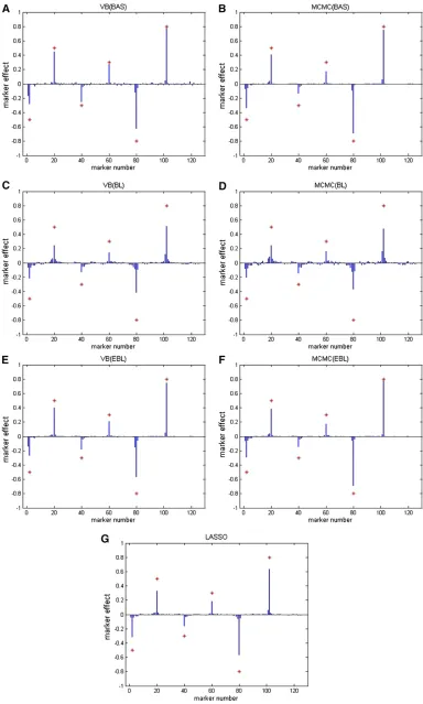
bjðj¼0; 1;. . .; pÞ represented the posterior mean esti-mates obtained from VB and MCMC methods or the ℓ1 -penalized least-squares estimates from the LASSO method. Note that for comparison, we also performed a standard LASSO analysis (Tibshirani 1996) by using the coordinate descent algorithm (Friedmanet al.2010) on the same data, where the LASSO shrinkage factor l was chosen so that the minimum of CVE was reached. These results are also presented in Table 1. Finally, the estimated QTL effects av-eraged over 50 replications for all the methods are shown in Figure 1.
From the perspective of producing the correct number of nonzero effects (i.e., QTL), VB-EBL performs best, because it is able to capture on average 5.50 trait loci, which is close to 6, and at the same time provides accurate estimates of QTL effects. VB-BL also estimates almost 6 trait loci correctly, but it overshrinks their QTL effects. VB-BAS tends to identify correct QTL and provides accurate effect estimates for them, but it also gives many spurious signals. Compared to the VB approaches, MCMC-BAS and MCMC-EBL behave equally well in the sense that they accurately estimate the QTL effects. However, the number of correctly identified QTL is much smaller, because the 95% credible intervals estimated from MCMC samples are wider than those from VB.
MCMC-Table 1 Average performance of eight methods in the simulation study with 50 replications
Method MSE CVE C I Cextension
VB-BAS 0.6598 (0.1051) 1.7512 (0.1197) 4.9800 7.6600 6.4800
MCMC-BAS 0.9518 (0.1295) 1.4939 (0.0903) 3.7200 0.5800 4.1600
VB-BL 0.7701 (0.1175) 1.5476 (0.0556) 4.6000 1.4200 5.7400
MCMC-BL 0.6481 (0.1189) 1.6279 (0.0755) 1.9400 0.0600 1.9800
VB-EBL 0.7960 (0.1097) 1.4401 (0.0626) 4.5800 1.3600 5.5000
MCMC-EBL 0.7412 (0.1156) 1.4648 (0.0625) 2.6800 0.0600 2.7200
LASSO 0.8461 (0.1552) 1.3694 (0.0463) 2.2600 0.0600 2.3200
Figure 1 (A–G) In the simulation
BL, similarly to VB-BL, tends to overshrink the QTL effects. Compared to the Bayesian methods, standard LASSO is able to shrink marker effects exactly to zero, but it is not able to provide confidence intervals. Thus, we implemented the phenotype permutation method to decide a 95% signifi-cance threshold, on the basis of which QTL were selected from the LASSO solution (Churchill and Doerge 1994). To perform a permutation test, the phenotypes were reshuffled to destroy the association between the phenotypes and the markers for 1000 runs. For each run, we estimated the marker effects and used the largest absolute effect to con-struct an empirical distribution. We used its 95% quantile as a threshold, so that a marker with the absolute effect larger than the threshold was considered to be a QTL. Results showed that 2.32 QTL on average were detected. Further-more, we also performed the permutation test for the three VB methods, and the results are summarized in Table 2. It seems that the permutation test performed well with VB-EBL. It correctly detected 3.72 QTL on average, which is less than the number of QTL detected by the credible intervals, but it also provided less falsely selected QTL. For VB-BAS, the estimated threshold was too high so that only 0.46 markers were detected to be the QTL on average. For VB-BL, the threshold was too low, and we obtained too many false positive signals. Moreover, MSE is often used to mea-sure the goodness-of-fit of the model to the data. From the results, it can be seen that MCMC-BL and VB-BAS have smaller MSE on average than others, meaning that theyfit the data better. On the other hand, cross-validation provides a measure of predictive ability for a method. Standard LASSO, MCMC-EBL, VB-EBL, and MCMC-BAS approaches tend to give smaller CVE, meaning that they have good pre-dictive ability. MCMC-BL and VB-BAS produced the highest CVEs, indicating that these two methods may suffer from overfitting in this replication study.
Analysis of simulated data to estimate epistatic effects A backcross data set with 600 individuals was simulated in Xu (2007). In this data set, 121 markers were evenly distributed through a single chromosome of 1800 cM. Simulated QTL with main effects were exactly placed on 9 markers, and 13 marker pairs were simulated to have interaction effects. Phenotypes were simulated as the cumulative sum of all main and pairwise interaction effects. The population mean and residual variance of normal distribution used in the simulation were 5.0 and 10.0,
respectively (the resulting heritability was 0.9065). See Xu (2007) for more details on these data.
We tested the efficiency of VB methods to estimate epistatic effects by using simulated backcross data from Xu (2007). Note that the same linear regression model pre-sented in (1) can also be used here. Design matrixXshould include not only 121 markers, but also1212
¼7260 pair-wise interaction terms between each possible pair of markers, which leads to an ill-posed (P?n) regression prob-lem. We implemented VB-BAS, VB-BL, and VB-EBL as well as MCMC-BAS, MCMC-BL, and MCMC-EBL (with the same gamma priors for d2 and h
j2 as in the previous example analysis) on these data. Here we use the same priors for the main and interaction effects. The 95% credible inter-vals-based criterion is also considered as the tool to judge the QTL for each method.
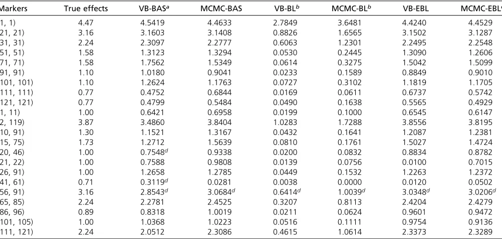
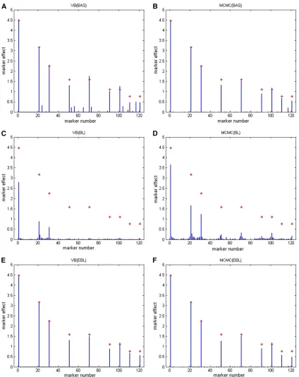
Results are summarized in Table 3 and Figures 2 and 3. For methods including VB-BAS, MCMC-BAS, VB-EBL, and MCMC-EBL, we conclude that their performance is good in general, because they are able to detect almost all the cor-rect loci with main effects as well as the interaction terms, and the estimated QTL effects are also accurate. VB-EBL, MCMC-EBL, and MCMC-BAS fail tofind an interaction effect at marker pair (41, 61). In addition, VB-EBL does notfind an effect at pair (21, 22). MCMC-EBL produced a quite accurate estimate of 0.7015 at (21, 22) that is close to the true effect size 1, but the pair (21, 22) is not recognized as a QTL by the interval test. Compared to the former three methods, VB-BAS is able tofind all the important signals, but tends to give many spurious signals in addition to the correct ones. Fi-nally, the results obtained from VB-BL and MCMC-BL are not satisfactory. They can detect only a few major QTL, and the estimated QTL effects in these positions are not accurate. Similar analysis has been done by using empirical Bayes, LASSO, penalized maximum likelihood (Zhang and Xu 2005), and SSVS in Xu (2007). Results obtained from our variational Bayes approaches including VB-EBL and VB-BAS are also competitive with the results published earlier.
Finally, we employed still two other efficient methods for detecting epistatic effects and compared them to our methods. The first one is an EM algorithm for estimat-ing epistatic effects introduced by Yi and Banerjee (2009). In summary, a Bayesian hierarchical model was proposed with priors bjjs2j Nð0;s2jÞ and s2j Inv2x2ðnj; s2jÞ
ðj¼1; . . . ; pÞ. Note that an inverse-x2distribution Inv–
x2(n, s2) is equivalent to an inverse gamma distribution Inv-Gammaðn= 2; ns2= 2Þ. If both n and s2 were set to be zero, we exactly obtain a BAS model. In our example, we chosen¼0.01 ands2¼0.0001, as Yi and Banerjee (2009) suggested. The method has been implemented in the re-cently developed R package BhGLM (http://www.ssg.uab. edu/bhglm/), which takes the advantage of R’s built-in
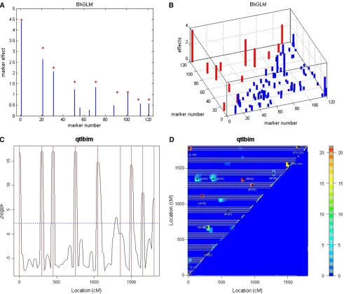
func-tion glm. We found that the method cannot be directly ap-plied to this data set due to the memory limitation of the computer. Alternatively, we used a model search strategy (with thresholds t1¼ 1028and t2 ¼0.1) also introduced
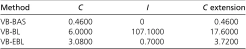
Table 2 Average performance of the permutation test to judge QTL signals for VB-BAS, VB-BL, and VB-EBL with 50 replications
Method C I Cextension
VB-BAS 0.4600 0 0.4600
VB-BL 6.0000 107.1000 17.6000
VB-EBL 3.0800 0.7000 3.7200
in Yi and Banerjee (2009), which gradually filters out the markers with negligible effects and therefore reduces the dimensionality of the model. The second method is a MCMC-based model-finding algorithm of Yi et al. (2005), which has been implemented in the R package qtlbim (see Yandell et al. 2007). We set the expected number of QTL with main effects (main.nqtl) to be 9, and the expected total number of QTL with both main and epistatic effects (mean. nqtl) to be 20 on the basis of the number of main and epistatic effects detected by VB-EBL. The results are shown in Figure 4. It seems that R/BhGLM does not provide as good results as VB-EBL. First of all, the locations of two main QTL, which were found at 88 and 113, are biased from the true locations 91 and 101. Second, many spurious QTL sig-nals were detected in R/BhGLM analysis. These may be mainly caused by the use of the model search strategy. A simultaneous estimation of all the markers and the interac-tion terms may lead to better results. On the other hand, R/ qtlbim seems to work nicely. Since the Bayesian model be-hind R/qtlbim assigned an indicator variable to each marker, an estimate of the Bayes factor can be derived from the MCMC samples and be used to judge the QTL positions. Results in Figure 4C indicate the markers with large values of Bayes factors were located either exactly at the positions of true main QTL or close to them. Furthermore, R/qtlbim was also able to correctly detect most of the marker pairs with true epistatic effects, as illustrated in Figure 4D. Like VB-EBL, R/qtlbim failed to detect the epistatic effects at marker pairs (21, 22) and (41, 61). In addition, it produces
a few false positive signals. We have also found that the performance of R/qtlbim relies on the choice of priors in-cluding main.nqtl and mean.nqtl. As we have shown, it is possible to set those priors on the basis of results from our VB methods.
Real barley data analysis
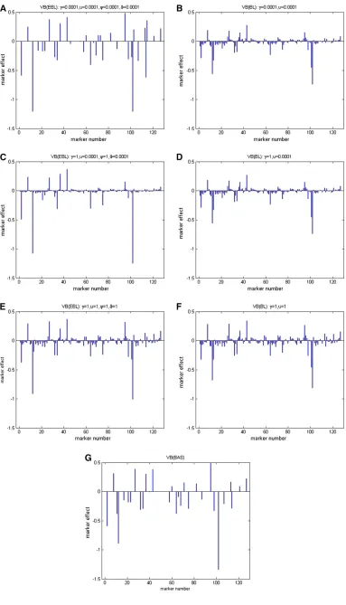
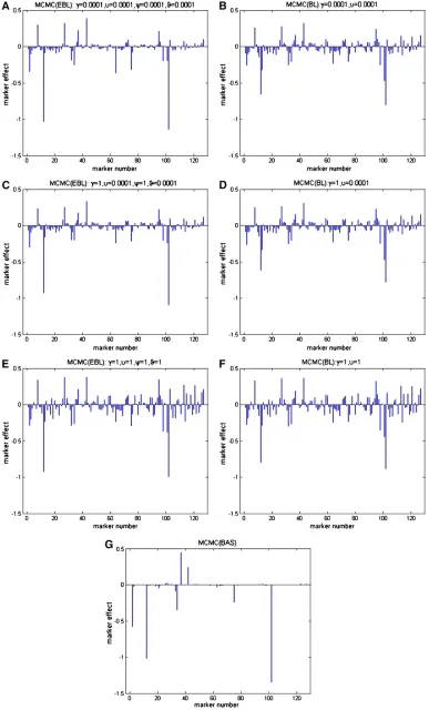
The mapping population consists of 145 doubled haploid lines (n¼145), each grown in a range of environments. A total of 127 markers were genotyped, covering 1270 cM of the barley genome, with the average distance between markers of 10.5 cM. Seven traits including yield, heading, maturity, height, lodging, kernel weight, and test weight were measured for each line.
Here we selected the kernel weight as the quantitative traits used in the analysis. Before the analysis, the pheno-type values for each line in the traits were averaged over the environments. Missing marker genotypes were imputed in the same way as in the first example analysis. The VB methods based on the three models as well as the corresponding MCMC approaches were used for the analy-sis. To test the prior sensitivity of VB-BL and VB-EBL, we implemented VB-BL with different combinations of hyper-parameters as (g1,n1) ¼(0.0001, 0.0001), (g2,n2) ¼(1, 0.0001), and (g3, n3) ¼ (1, 1), respectively. Correspond-ingly, for VB-EBL, we chose (g1,n1)¼(c1,q1)¼(0.0001, 0.0001), (g2,n2)¼(c2,q2)¼(1, 0.0001), and (g3,n3)¼ (c3,q3) ¼(1, 1). In MCMC-EBL and MCMC-BL, we used the same priors as in the corresponding VB approaches.
Table 3 Estimated main and interaction effects from VB-BAS, MCMC-BAS, VB-BL, MCMC-BL, VB-EBL, and MCMC-EBL for the backcross data originally simulated by Xu (2007)
Markers True effects VB-BASa MCMC-BAS VB-BLb MCMC-BLb VB-EBL MCMC-EBLc
(1, 1) 4.47 4.5419 4.4633 2.7849 3.6481 4.4240 4.4529
(21, 21) 3.16 3.1603 3.1408 0.8826 1.6565 3.1502 3.1287
(31, 31) 2.24 2.3097 2.2777 0.6063 1.2301 2.2495 2.2548
(51, 51) 1.58 1.3123 1.3294 0.0530 0.2445 1.3090 1.2606
(71, 71) 1.58 1.7562 1.5349 0.0614 0.3275 1.5042 1.5099
(91, 91) 1.10 1.0180 0.9041 0.0233 0.1589 0.8849 0.9010
(101, 101) 1.10 1.2624 1.1763 0.0727 0.3102 1.1819 1.1705
(111, 111) 0.77 0.4752 0.6844 0.0169 0.0611 0.6737 0.5742
(121, 121) 0.77 0.4799 0.5484 0.0490 0.1638 0.5565 0.4929
(1, 11) 1.00 0.6421 0.6958 0.0199 0.1000 0.6545 0.6147
(2, 119) 3.87 3.4860 3.8404 1.0283 1.7288 3.8556 3.8195
(10, 91) 1.30 1.1521 1.3167 0.0432 0.1641 1.2087 1.2381
(15, 75) 1.73 1.2712 1.5639 0.0810 0.1761 1.5027 1.4724
(20, 46) 1.00 0.7548d 0.9338 0.0200 0.0832 0.8834 0.8782
(21, 22) 1.00 0.7588 0.9808 0.0139 0.0756 0.0100 0.7015
(26, 91) 1.00 1.2658 1.2785 0.0449 0.1532 1.2263 1.2372
(41, 61) 0.71 0.3119d 0.0281 0.0038 0.0000 0.0120 0.0502
(56, 91) 3.16 2.8543d 3.0684d 0.6414d 1.0039d 3.0348d 3.0206d
(65, 85) 2.24 2.2781 2.4525 0.3207 0.8113 2.4204 2.4279
(86, 96) 0.89 0.8318 1.0019 0.0211 0.0624 0.9601 0.9472
(101, 105) 1.00 1.0368 1.0223 0.0516 0.1111 0.9754 0.9136
(111, 121) 2.24 2.0512 2.3086 0.4615 1.0614 2.3373 2.3289
aIn addition to those reported, VB-BAS detects 307 spurious QTL signals.
bFor both VB-BL and MCMC-BL, markers (or marker pairs) (1, 1), (21, 21), (31, 31), (2, 119), (56, 90), (65, 85), and (111, 121) are judged as QTL on the basis of the 95%
credible interval test.
cFor MCMC-EBL, marker pair (21, 22) is not judged as a QTL on the basis of the 95% credible interval test.
Together with VB-BAS, results of VB estimation are pre-sented in Figure 5. Additionally, results of MCMC estimation are shown in Figure 6. We see that the VB-EBL is quite sensitive to the choices of the hyperparameters. By our pref-erable choice of shape parameter as 1 and rate parameter as 0.0001, VB-EBL tends to produce a relatively sparse model compared to the other two choices. On the other hand, VB-BL seems to be less sensitive to the choice of the
hyperpara-meters. We also note the difference between the results obtained from VB and MCMC methods. For example, in the BAS model, the MCMC approach leads to a sparser model than the VB approach. Another interesting feature is that the credible interval estimated from VB methods tends to be narrower than the one estimated from the MCMC samples based on the same shrinkage model. Figure 7 shows an example, where we plot the estimated effects of
markers (in blue) which are announced to be significant (95% credible intervals do not contain zero) from VB-EBL. The corresponding posterior means and 95% C.I.’s estimated by MCMC (in red) are also shown in Figure 7. Clearly, all the MCMC-derived 95% C.I.’s contain VB-derived 95% C.I.’s. Consequently, from VB, we obtain 12 QTL by interval infer-ence, but from MCMC, only 3 of them including markers 12, 43, and 102 are claimed to be significant. This implies that, in practice, the VB inference based on intervals may tend to give more false positive results. Alternatively, we performed a permutation test with VB-EBL, and three markers, 2, 12,
and 102 were found to be significant. These markers are located close to the QTL signals reported in Tinker et al. (1996).
Discussion
We propose a variational Bayes approximation-based algo-rithm for Bayesian shrinkage analysis of multiple-QTL mapping. Because of the usage of the conjugate priors, iterative algorithms can be easily derived for hierarchical Bayesian shrinkage models including BAS, BL, and EBL to
update the approximate marginal distribution of each parameter. Compared to MCMC methods, which are used to generate dependent samples from the target posterior distribution directly, VB seeks an approximate distribution in a factorized form that has minimum KL divergence to the target posterior. Therefore, it is not surprising that for a particular model, the posterior mean estimated by MCMC can be different from that estimated by VB. Another feature is that the credible intervals estimated by VB methods are narrower than those of MCMC. Therefore, if the credible intervals are used to judge QTL, VB tends to give more false positive signals. On the other hand, MCMC-based shrinkage methods tend to provide too large credible intervals arguably due to the collinearity between loci, and a criterion
based on these may fail to find some true QTL signals. Therefore, we suggest that a credible intervals-based crite-rion should be used for QTL detection only in thefirst stage. A further method may be needed to judge QTL in a more accurate way in the second stage. We found that a permu-tation-based test might be a suitable tool to control false positivefindings under the VB-EBL model, but not for VB-BL and VB-BAS. However, performing such a test often requires huge computation time and is not preferable for the high-dimensional data. As Heaton and Scott (2010) pointed out, how to select the significant variables under a Bayesian shrinkage procedure remains an open problem and needs to be investigated in further studies. Compared to the MCMC approaches, one major advantage of VB approaches is their
computational efficiency. Note that the computation time for a single iteration in VB is approximately identical to a Gibbs sampling step. On the basis of our empirical experiments, VB algorithms need 100–1500 iterations until convergence. On the other hand, when MCMC is used, we usually need to draw .10,000 MCMC samples to obtain good posterior summaries. Therefore, compared to MCMC, VB methods re-quire much less computation time. Table 4 presents a com-parison of the computation time of both VB and MCMC in our second and third example analyses. All the methods were implemented in MATLAB on a regular desktop with a 3.00-GHz Intel Pentium 4 processor and 3 GB RAM. The MATLAB source code is available in File S2.
The VB method we consider here can be regarded as an extension of the well-known EM algorithm and can be applied to a broader class of Bayesian models. In an EM algorithm, when the hidden variables interact with each other and their joint full conditional distribution is not analytically available, the variational approximation may be applied as an alternative to proceed to the E-step. This is then called the VB-EM algorithm (Beal 2003). Furthermore, if the parameters, with respect to which the objective func-tion is maximized, are considered as the hidden variables so that only the E-step is remaining, then we exactly obtain the VB algorithm mentioned in this article. More information about the connection between VB and EM algorithms is pro-vided inFile S1.
This article discusses three Bayesian shrinkage models, including BL, EBL, and BAS. BL and EBL can be regarded as the same model class, which uses double exponential prior
distributions of marker effects. Compared to BL, an impro-vement in EBL is to assign a marker-specific shrinkage factor hj to each marker in addition to a global shrinkage factor d. Mutshinda and Sillanpää (2010) pointed out that, by using this marker-specific shrinkage factor, EBL is able to relax the penalty for the important marker effects and mean-while push the unimportant marker effects strongly toward zero. From the results of our example analyses, it can be seen that VB-EBL outperformed VB-BL. In our simulated examples, VB-EBL gave accurate estimates of the marker effects and meanwhile produced a relatively sparse model. On the other hand, VB-BL tended to shrink the large marker effects too much, so that the estimation was biased. BAS, a third model we focused on, comes from a different model class, where the Student’stprior is assigned for the marker effects. In the simulation studies, we found that VB-BAS can produce accurate estimates of the marker effects, but the resulting model was not sparse compared to VB-EBL [with our default hyperparameters (g,n)¼(c,q)¼(1, 0.0001)], meaning that some spurious signals were present. There-fore, VB-BAS may not be a preferable method for QTL map-ping, in which we are more interested in detecting QTL with relatively large effects on the traits.
The Bayesian LASSO method has also been used for predicting phenotypic values and breeding values (De Los Camposet al.2009; Legarraet al.2011). In thefirst repli-cation study, we used cross-validation to measure the pre-dictive ability of our proposed methods, and we found that the performance of VB-EBL is competitive to LASSO, which has been widely used for prediction problems in many areas. However, the predictive performance of a certain method depends on the property of data sets, i.e., the distribution of QTL effects (Daetwyleret al.2010; Clarket al.2011). The general predictive abilities of our VB methods need to be investigated in more complicated data sets.
In addition, it is necessary to point out the difference between our EBL and BL models and other approaches. Compared to Mutshinda and Sillanpää (2010), we used dif-ferent parameterizations and priors of the shrinkage factors in the EBL and BL models. Taking the EBL model as an example, in Mutshinda and Sillanpää (2010),dandhjwere treated as parameters, and they were assigned the uniform priors Uni(0, 100). However, in our VB approaches,d2and
h2j are treated as parameters, and conjugate priors d2 Gamma(g,n) andh2j Gamma(c,q) are used to guarantee the convenience of the computation. For comparison, here we used the same gamma priors for MCMC as in the VB approaches. However, on the basis of our empirical experi-ments, EBL is sensitive to the hyperparameters with the
Figure 7 A comparison between 95% credible intervals estimated from VB (in blue) and MCMC (in red).
Table 4 Comparison of the approximate computation time (scaled in seconds) of VB and MCMC methods for the barley (p¼127,n¼145) and simulated data by Xu (2007) (p¼7260,n¼600)
Data size VB-BAS VB-BL VB-EBL MCMC-BAS MCMC-BL MCMC-EBL
p¼127,n¼145 4.05 0.48 0.72 111.50 112.85 114.66
gamma priors in MCMC, and the use of the uniform priors suggested by Mutshinda and Sillanpää (2010) might be a good choice to avoid tuning.
In BL and EBL, another remaining issue is“unimodality”. To guarantee unimodality of the posterior, Park and Casella (2008) suggested the incorporation of the global residual variance s2
0into the prior distribution of marker effects as
bjN(0,s20sj2). They demonstrated that, by doing this, the posterior distribution has a unique mode (maximum value), and the corresponding MCMC algorithm may converge faster. However, in VB estimation, instead of the posterior mode, we seek the minimum value of the KL divergence between the factorized approximate distribution and the original posterior. Thereby, the model suggested by Park and Casella (2008) may not be optimal for our variational Bayes approach. In fact, we found that the VB algorithm based on the Park and Casella model even slowed down the convergence. Also note that the uniqueness of the min-imization (i.e., convergence to a global minimum) of the KL divergence in VB estimation is not guaranteed in general (see Šmídl and Quinn 2006). Further investigation may be needed to check for uniqueness of the VB approximation.
Finally, we point out some weaknesses of our current VB approach, which can potentially be improved in future work. First, we derived the approximate marginal distribution for each marker effectbjseparately. During the approximation, the posterior correlations among marker effectsbjare lost. It may be beneficial to take all marker effects as a blockb¼
[b1,. . .,bp] and update them simultaneously. This may help to reduce the minimum value of KL divergence and may give a better approximation to the target posterior distribution. In practice, this involves the inversion of a p · p matrix
ðE½t2 0X
TXþ
diagðEðt2ÞÞÞ21
; where Eðt2Þ ¼ ½Eðt2 1Þ;. . .; Eðt2
pÞ; which is demanding in terms of computation and storage when p is large. This problem can be potentially solved by applying“Woodbury matrix identity”(Woodbury 1950), which can be applied to convert thep·pmatrix into ann·none, so that the dimension of the matrix is reduced significantly. Second, in VB-EBL and VB-BL, we used gamma priors for shrinkage factors and chose shape parameters to be 1 and rate parameters to be a small value (say 0.0001) so that the priors were flat. This strategy was successful throughout our example analyses here, but may not be the optimal choice in general, since these methods are quite sensitive to the choice of the gamma parameters (see our third example analysis). A first solution to this problem might be that we perform a prior sensitivity analysis using cross-validation for new data to give optimal models on the basis of different data sets. Second, we have found that in the formula to update qðh2
jjyÞðj¼1; :::;pÞ (in step VI in the Appendix), if we heuristically replace E½1=t2
j by 1= E½t2j ¼1= m, VB-EBL can produce equally good results, and these slight modifications seem to make VB less sensitive to hyperparameters, although they do not have any theoretical justification. Logsdon et al. (2010) also made some slight modifications in their VB algorithm to maintain the ease of
computation, and they stated that those modifications did not significantly affect the results. However, in this article, we have presented only the results from standard VB.
Acknowledgments
We are grateful to Petri Koistinen for giving constructive comments on the manuscript. This work was supported by the Finnish Graduate School of Population Genetics and by research grants from the Academy of Finland and the University of Helsinki’s Research Funds.
Literature Cited
Armagan, A., 2009 Variational bridge regression, pp. 17–24 in 12th International Conference on Artificial Intelligence and Statis-tics, edited by D. van Dyk and M. Welling. Clearwater Beach, Florida.
Beal, M. J., 2003 Variational algorithms for approximate Bayesian inference. Ph.D. Thesis, University of London, London. Bishop, C. M., 2006 Pattern Recognition and Machine Learning.
Springer-Verlag, New York.
Broman, K. W., and T. P. Speed, 2002 A model selection approach for the identification of quantitative trait loci in experimental crosses. J. R. Stat. Soc. B 64: 641–656.
Churchill, G. A., and R. W. Doerge, 1994 Empirical threshold values for quantitative trait mapping. Genetics 138: 963–971. Clark, S. A., J. M. Hickey, and J. H. J. Van Der Werf,
2011 Different models of genetic variation and their effect on genomic evaluation. Genet. Sel. Evol. 43: 18.
Daetwyler, H. D., R. Pong-Wong, B. Villanueva, and J. A. Woolliams, 2010 The impact of genetic architecture on genome-wide eval-uation methods. Genetics 185: 1021–1031.
De los Campos, G., H. Naya, D. Gianola, J. Crossa, A. Legarraet al., 2009 Predicting quantitative traits with regression models for dense molecular markers and pedigree. Genetics 182: 375–385. Figueiredo, M. A. T., 2003 Adaptive sparseness for supervised learning. IEEE Trans. Pattern Anal. Mach. Intell. 25: 1150– 1159.
Friedman, J., T. Hastie, and R. Tibshirani, 2010 Regularization paths for generalized linear models via coordinate descent. J. Stat. Softw. 33: 1.
Gelman, A., J. B. Carlin, H. S. Stern, and D. B. Rubin, 2004 Bayesian Data Analysis, Ed. 2. Chapman & Hall, London. Grimmer, J., 2011 An introduction to Bayesian inference via
var-iational approximations. Polit. Anal. 19: 32–47.
George, E. I., and R. E. McCulloch, 1993 Variable selection via Gibbs sampling. J. Am. Stat. Assoc. 88: 881–889.
Habier, D., R. L. Fernando, and J. C. M. Dekkers, 2007 The impact of genetic relationship information on genome-assisted breeding values. Genetics 177: 2389–2397.
Haley, C. S., and S. A. Knott, 1992 A simple regression method for mapping quantitative trait loci in line crosses using flanking markers. Heredity 69: 315–324.
Hastie, T., R. Tibshirani, and J. Friedman, 2009 Elements of Sta-tistical Learning, Ed. 2. Springer-Verlag, New York.
Heaton, M., and J. Scott, 2010 Bayesian computation and the linear model, pp. 527–545 in Frontiers of Statistical Decision Making and Bayesian Analysis, Chap. 14, edited by M. H. Chen, D. K. Dey, P. Müller, D. Sun, and K. Ye. Springer-Verlag, New York.
Jaakkola, T. S., and M. I. Jordan, 2000 Bayesian parameter esti-mation via variational methods. Stat. Comput. 10: 25–37. Kass, R. E., and A. Raftery, 1995 Bayes factors. J. Am. Stat. Assoc.
90: 773–795.
Knürr, T., E. Läärä, and M. J. Sillanpää, 2011 Genetic analysis of complex traits via Bayesian variable selection: the utility of a mixture of uniform priors. Genet. Res. 93: 303–318. Kullback, S., and R. A. Leibler, 1951 On information and suffi
-ciency. Ann. Math. Stat. 22: 79–86.
Legarra, A., C. Robert-Granié, P. Croiseau, F. Guillaume, and S. Fritz, 2011 Improved Lasso for genomic selection. Genet. Res. 93: 77–87.
Li, J., K. Das, G. Fu, R. Li, and R. Wu, 2011 The Bayesian LASSO for genome-wide association studies. Bioinformatics 27: 516– 523.
Logsdon, B. A., G. E. Hoffman, and J. G. Mezey, 2010 A varia-tional Bayes algorithm for fast and accurate multiple locus genome-wide association analysis. BMC Bioinformatics 11: 58.
Meuwissen, T. H. E., B. J. Hayes, and M. E. Goddard, 2001 Pre-diction of total genetic value using genome-wide dense marker maps. Genetics 157: 1819–1829.
Mutshinda, C. M., and M. J. Sillanpää, 2010 Extended Bayesian LASSO for multiple quantitative trait loci mapping and unob-served phenotype prediction. Genetics 186: 1067–1075. O’Hara, R. B., and M. J. Sillanpää, 2009 A review of Bayesian
variable selection methods: What, how, and which? Bayesian Anal. 4: 85–118.
Parisi, G., 1988 Statistical Field Theory. Addison-Wesley, New York.
Park, T., and G. Casella, 2008 The Bayesian LASSO. J. Am. Stat. Assoc. 103: 681–686.
Robert, C. P., and G. Casella, 2004 Monte Carlo Statistical Meth-ods, Ed. 2. Springer-Verlag, New York.
Seshadri, V., 1999 The Inverse Gaussian Distribution. Springer-Verlag, New York.
Sillanpää, M. J., 2009 Detecting interactions in association studies by using simple allele recoding. Hum. Hered. 67: 69–75.
Sillanpää, M. J., and M. Bhattacharjee, 2005 Bayesian associa-tion-based fine mapping in small chromosomal segments. Ge-netics 169: 427–439.
Sillanpää, M. J., and J. Corander, 2002 Model choice in gene mapping: what and why. Trends Genet. 18: 301–307.
Šmídl, V., and A. Quinn, 2006 The Variational Bayes Method in Signal Processing. Springer-Verlag, New York.
Sun, W., J. G. Ibrahim, and F. Zou, 2010 Genomewide multiple-loci mapping in experimental crosses by iterative adaptive pe-nalized regression. Genetics 185: 349–359.
Tibshirani, R., 1996 Regression shrinkage and selection via the lasso. J. R. Stat. Soc. B 58: 267–288.
Tinker, N. A., D. E. Mather, B. G. Rossnagel, K. J. Kasha, A. Kleinhofs et al., 1996 Regions of the genome that affect agronomic per-formance in two-row barley. Crop Sci. 36: 1053–1062. Tipping, M. E., 2001 Sparse Bayesian learning and the relevance
vector machine. J. Mach. Learn. Res. 1: 211–244.
Tzikas, D. G., A. C. Likas, and N. P. Galatsanos, 2008 The varia-tional approximation for Bayesian inference. IEEE Signal Pro-cess. Mag. 25: 131–146.
Woodbury, M., 1950 Inverting modified matrices. Technical Re-port 42. Statistical Research Group, Princeton University, Prince-ton, NJ.
Xu, S., 2003 Estimating polygenic effects using markers of the entire genome. Genetics 163: 789–801.
Xu, S., 2007 An empirical Bayes method for estimating epistatic effects of quantitative trait loci. Biometrics 63: 513–521. Xu, S., 2010 An expectation–maximization algorithm for the
Lasso estimation of quantitative trait locus effects. Heredity 105: 483–494.
Yandell, B. S., T. Mehta, S. Banerjee, D. Shriner, R. Venkataraman et al., 2007 R /qtlbim: QTL with Bayesian Interval Mapping in experimental crosses. Bioinformatics 23: 641–643.
Yi, N., and S. Banerjee, 2009 Hierarchical generalized linear mod-els for multiple quantitative trait locus mapping. Genetics 181: 1101–1113.
Yi, N., and S. Xu, 2008 Bayesian LASSO for quantitative trait loci mapping. Genetics 179: 1045–1055.
Yi, N., V. George, and D. B. Allison, 2003 Stochastic search vari-able selection for identifying multiple quantitative trait loci. Ge-netics 164: 1129–1138.
Yi, N., B. S. Yandell, G. A. Churchill, D. B. Allison, E. J. Eisenet al., 2005 Bayesian model selection for genome-wide epistatic quantitative trait loci analysis. Genetics 170: 1333–1344. Zhang, Y.-M., and S. Xu, 2005 A penalized maximum likelihood
method for estimating epistatic effects of QTL. Heredity 95: 96–104. Zhang, M., K. L. Montooth, M. T. Wells, A. G. Clark, and D. Zhang, 2005 Mapping multiple quantitative trait loci by Bayesian clas-sification. Genetics 169: 2305–2318.
Zou, H., 2006 The adaptive lasso and its oracle properties. J. Am. Stat. Assoc. 101: 1418–1429.
Appendix: VB Estimation Algorithm for Extended Bayesian LASSO
First, the logarithm of the joint distribution of parameters and data is
lnpðu;yÞ ¼pb0;b1; :::;bp;t20;t21; :::;t2p;d2;h21; :::;h2py
¼
2 4n
2lnt 2 02 t2 0 2 Xn
i¼1
0
@yi2b02
Xp
j¼1 xijbj
1 A
23
5þ 2lnt2
0 þ 2 41 2 Xp
j¼1 ln t2
j2 1 2
Xp
j¼1
t2 jb2j
3 5
þ
2 4plnd2þPp
j¼1 ln h2
j22
Pp j¼1
ln t2 j2
1 2
Xp
j¼1
d2h2 j t2
j
3
5þ ðg21Þlnd22nd2
þ
"
ðc21ÞPp j¼1
ln h2 j2q
Pp j¼1
h2 j
#
þC;
(A1)
whereCis a constant. Next, we start to derive the VB mar-ginal distributions ^qð•jyÞ for parameters b0; b1;. . .;bp;
t2
0; t21;. . .;t2p; d 2; h2
1;. . .; h2p on the basis of Equation 10.
I. Derivation ofq^ðb0jyÞ
By keeping only terms containingb0, we obtain
ln^qðb0jyÞ}E^qðu=b0jyÞ½lnpðu;yÞ
¼2Et20
2 8 < :nb2022b0
Xn
i¼1
0 @yi2
Xp
j¼1 xijE½bj
1 A 9 = ;þC;
(A2)
where ^qðu= b0jyÞ represents the product of all other ap-proximate marginal distributions except ^qðb0jyÞ. Here E[•] is a simplified notation of the expectation of the pa-rameter • with respect to its approximate marginal dis-tribution ^qð•jyÞ [i.e., E½t20 is a simplified notation of
E^qðt2 0jyÞ½t
2 0 ¼
RN 0 t
2 0^qðt
2 0jyÞdt
2
0Þ], and C represents those terms that do not contain b0. We can recognize from (A2) that^qðb0jyÞis anormal distributionwith mean
E½b0 ¼ 1 n
Xn
i¼1 0 @yi2Xp
j¼1 E h bj i xij 1 A (A3) and variance
Var½b0 ¼ 1 n
1
Et20: (A4)
To update E[b0] and Var[b0], we need to calculate E[bj] andE½t20on the basis of approximate marginal distributions
^
qðbjjyÞðj¼1;. . .;pÞ and ^qðt20jyÞ, respectively, which are shown in the following.
II. Derivation of ^qðbj j yÞðj¼1;. . .;pÞ
Following a similar procedure to that in (1), we have
ln^q
bjy
}E^qðu=b
jjyÞ½lnpðu;yÞ
¼21 2 E t
2 0
Xn
i¼1 xi2 jþE
h
t2j
i!
b2j
þbjEt20X n
i¼1
yi2E½b02 X
k6¼j
E½bkxi k
xi jþC;
(A5)
showing that^qðbjjyÞis also anormal distributionwith mean
E½bj ¼E½t20X
n
i¼1
x2i jþE½t2j
21 E½t20X
n
i¼1
yi2E½b02
X
k6¼j E½bkxi k
xi j
(A6)
and variance
Var½bj ¼ ðE½t20 Xn
i¼1
x2i jþE½t2jÞ21: (A7)
In addition, the expectation ofbj2(second moment) can be calculated by E[bj2] = E[bj]2 + Var[bj], which is needed later.
III. Derivation of ^qðt20 j yÞ
We have
ln^qt20jy}E^qðu=t2 0yÞ
½lnpðu;yÞ
¼ ða121Þlnt202 b1
2t 2 0þC;
(A8)
where
a1¼n
2; (A9)
and
b1¼
Pn
i¼1ðyi2E½b02
Pp
j¼1E½bjxi jÞ2þVar½b0 þ
Pn i¼1
Pp
j¼1x2i jVar½bj
2 :
(A10)
Here ^qðt20 j yÞ is recognized as a gamma distribution with parameters shape parameter a1 and rate parameter b1. In addition, we need to calculate the meanE½t20 j y ¼a
1= b1to update other approximate distributions.
IV. Derivation ofq^ðt2j j yÞ( j = 1, . . . , p) ln^qðt2jjyÞ}E^qðu=t2
jyÞ
½lnpðu;yÞ
¼23 2lnt
2
j 2 1 2E½b
2
jt2j 2 1 2
E½d2E½h2j
t2j þC:
(A11)
Here^qðt2
m¼
ffiffiffiffiffiffiffiffiffiffiffiffiffiffiffiffiffiffiffiffiffi E½d2E½h2j
E½b2j
v u u
t (A12)
and
lj¼Ed2
E
h
h2j
i
: (A13)
Note that a general form of the inverse Gaussian density is
pðx j m;lÞ ¼l 2p
1=2
x2ð3=2Þexph2lð2mx22mxÞ2
i
ðx.0;m.0;l.0Þ: (A14) To update other approximate distributions, we need to obtain the expectation of t2j as E½t2j ¼m, as well as the expectation of 1= t2j asE½1= t2j ¼1= mþ1= lj.
V. Derivation of^qðd2jyÞ
ln^qd2jy}E^qðu=d2jyÞ½lnpðu;yÞ
¼ ðpþg21Þlnd22
1 2
Xp
j¼1 Eh2jE
1
t2j
þn
d2þC:
(A15)
Here ^qðd2 j yÞ is recognized as a gamma distribution with shape parameter
a2¼pþg (A16)
and rate parameter
b2¼1 2
Xp
j¼1 E½h2jE
h1
t2j
i
þn: (A17)
We also need the expectationE½d2 ¼a2 = b2.
VI. Derivation ofq^ðh2
j j yÞ(j = 1, . . . , p) ln^qðh2j j yÞ}Eq^ðu=h2
jyÞ
½lnpðu;yÞ
¼clnh2j 2
1 2Ed
2 E
1
t2j
þq
h2j þC:
(A18)
Thus, ^qðh2j j yÞ is also a gamma distribution with shape parameter
a3j¼1þc (A19)
and rate parameter
b3j¼ 1 2E½d
2E
1
t2j
þq: (A20)
The expectationE½h2
j ¼a3j= b3jalso needs to be calculated. To update the approximate distributions inAppendix sec-tions I–VI successively, we need tofirst assign initial values to the required expectations. In practice, we use E[bj] ¼ 0 (j¼0, 1, . . . , p),E½t2
j52 (j¼0, 1, . . . ,p),E[d2]¼ 1, and E½h2
j51 (j ¼ 0, 1, . . . , p). In addition, we can derive the lower bound as
L¼2n2p21
2 lnð2pÞ þ 2pþ1
2 2pln 22 Pp
j¼1E½b 2
jE½t2j
2 þ
ln Var½b0
2 þX
p
i¼1
ln Var½bj
2 þln
ng GðgÞþ pln
qc
GðcÞ2a1lnb1þlnGða1Þ
2
Pp j¼1ln lj
2 2 a2lnb2þlnGða2Þ2 Xp
j¼1
½a3jlnb3j2lnGða3jÞ
þ12X p
j¼1
E½d2E½h2jEh1
t2
j i
;
(A21)
whereG(•) is the gamma function.
Finally, after convergence, we obtain an approximate distribution for each marker effect. The mean E[bj] can be regarded as a point estimate of the effect of marker j, and its 1 –apercent credible interval can be defined as
ðE½bj2
ffiffiffiffiffiffiffiffiffiffiffiffiffiffi Var½bj q
Qða = 2Þ;E½bj þ
ffiffiffiffiffiffiffiffiffiffiffiffiffiffi Var½bj q
GENETICS
Supporting Information http://www.genetics.org/content/suppl/2011/10/31/genetics.111.134866.DC1
Estimation of Quantitative Trait Locus Effects
with Epistasis by Variational Bayes Algorithms
Zitong Li and Mikko J. SillanpääSupporting Information
Estimation of Quantitative Trait Locus Effects with Epistasis by Variational
Bayes Algorithms
Zitong Li and Mikko J. Sillanpää
October 21, 2011
1 Connection between VB and EM
The VB method we consider in the paper is closely related to the well known EM algorithm. According to TZIKAS et al. (2008), the principle of EM algorithm for the MAP estimation problem θˆ = arg max
θp(θ|data) can be interpreted as follows: First of all, the log posterior distribution can be decomposed as
lnp(θ|data) =
!
q(z) lnp(θ,z|data)
q(z) dz−
!
q(z) lnp(z|θ,data)
q(z) dz
≡ L(q(z)) +KL(q(z)||p(z|θ,data)), (1.1) where z = {z1, ..., zm} are the hidden variables (to be integrated out), which are not of main interest, but are helpful to estimate the value of parametersθ. q(z)is a free selected
distribu-tion forz. Since KL(q(z)||p(z|θ,data))≥0,L(q(z))can be viewed as a lower bound of the log
posteriorlnp(θ|data). Denote the current value ofθasθOLD. In the E-step, the lower bound is
maximized with respect to the distributionq(z), which leads toq(z) =p(z|θOLD,data). In the
M-step, the lower bound withq(z)substituted byp(z|θOLD,data)is maximized with respect to
θ, which leads to a new estimation ofθasθNEW. By implementing these two steps successively,
the value of log posterior function increases, and eventually reaches its maximum.
An easy implementation of the EM algorithm requires the full conditional distributionp(z|θ,data)
to be explicitly known. However, in many models, hidden variables may interact with each other, and p(z|θ,data)becomes too complicated to be used in EM. One solution is to implement the
variational approximation method in the E-step, that is, the distributionq(z)is assumed to be
of the factorized formq(z) ="mi=1q(zi). Next, the lower bound can be maximized with respect
toq(zi) (i= 1,2, .., m). This procedure has been called variational EM (see BEAL 2003).
Fur-thermore, it is possible to consider the parametersθas a part of hidden variables, and implement a variational algorithm with only the E-step. This is exactly the same VB method introduced in the paper. Therefore, variational Bayes and variational EM can be viewed as extensions of
1
File S1
Supporting Information
traditional EM algorithm, and can be applied to a broader class of Bayesian models.
2 VB estimation algorithm for Bayesian Adaptive
Shrink-age
The priors are specified as
p(β0)∝1, (2.1)
p(τ2 0)∝
1
τ2 0
, (2.2)
p(βj|τj2)∝N(βj|0, 1
τ2
j
), (2.3)
p(τj2)∝
1
τ2
j
, (2.4)
and the logarithm of the joint distribution of parameters and data is
lnp(θ,y) = p(β0,β1, ...,βp,τ02,τ12, ...,τp2|y)
= [n
2lnτ
2 0 − τ2 0 2 n ! i=1
(yi−β0−
p
!
j=1
xijβj)2] + [−lnτ02] + [
1 2
p
!
j=1
lnτj2−
1 2
p
!
j=1 τj2β2j]
+[−
p
!
j=1
lnτ2
j] +C, (2.5)
whereC is a constant. Similarly as in VB-EBL, we can derive the VB marginal distributions
ˆ
q(•|y)for parametersβ0,β1,· · ·,βp,τ02,τ12,· · ·,τp2 in VB-BAS:
(I) Derivation ofqˆ(β0|y): qˆ(β0|y)is recognized as anormal distributionwith mean
E[β0] =
1
n
n
!
i=1
(yi−
p
!
j=1
E[βj]xij), (2.6)
and variance
Var[β0] = 1 n
1
E[τ2 0]
. (2.7)
(II) Derivation ofqˆ(βj|y): q(βj|y)is also anormal distribution, with mean
E[βj] = (E[τ02]
n
!
i=1
x2ij+E[τj2])−1E[τ02]
n
!
i=1
(yi−E[β0]−
!
k"=j
E[βk]xik)xij, (2.8)
and variance
Var[βj] = (E[τ02]
n
!
i=1
x2ij+E[τj2])−1, (2.9)

![Figure 3 The absolute value of estimated interacting effects [blue (effects aresimulated interacting effects (red solid lines on the left) from (A) VB-BAS, (B) MCMC-BAS, (C) VB-BL, (D) MCMC-BL, (E) VB-EBL, and (F) MCMC-EBL in .0.1) and green (effects are ,0.1) solid lines on the right] compared todata from Xu (2007).](https://thumb-us.123doks.com/thumbv2/123dok_us/1565583.1192417/11.603.91.514.41.528/absolute-estimated-interacting-effects-effects-aresimulated-interacting-compared.webp)