Measuring dinitrogen gas emissions from a lagoon treatment system

ABSTRACT

LARSEN, JULIE MELISSA. Measuring dinitrogen gas emissions from a lagoon treatment system. (Under the direction of John Classen, Sarah Liehr)

A method for collecting dinitrogen gas emissions from open pond waste treatment systems was developed. The method was critically tested in a laboratory for sources of air contamination to ensure reliable gas measurements. A laboratory experiment was done to estimate the rate at which dissolved dinitrogen would be stripped out of solution due to non-dinitrogen bubbles rising through the water column. A volumetric mass transfer coefficient for the process was estimated for clean water. The gas collection method was implemented in a partially aerated lagoon treatment system for dinitrogen and methane gas sampling. The volumetric mass transfer coefficient found in the laboratory for clean water was adjusted to compensate for field gas production rates, temperatures and wastewater quality to estimate the rate of stripped dinitrogen from the partially aerated lagoon. The estimated rate of stripped dinitrogen was subtracted from the total measured dinitrogen flux to estimate the dinitrogen produced biologically. Results from laboratory testing revealed that dinitrogen can be measured with low amounts of dinitrogen atmospheric contamination (0.57% N2) and

MEASURING DINITROGEN GAS EMISSIONS FROM A LAGOON TREATMENT SYSTEM

By

JULIE MELISSA LARSEN

A thesis submitted to the Graduate Faculty of North Carolina State University

in partial fulfillment of the requirements for the Degree of

Master’s of Science

BIOLOGICAL AND AGRICULTURAL ENGINEERING

Raleigh 2003

APPROVED BY:

__________________________

BIOGRAPHY

ACKNOWLEDGEMENTS

Many people have contributed to this research project and I would like to acknowledge and thank them for their support. My advisors Dr. Classen, Dr. Sarah Liehr and Dr. Wayne Robarge have helped me tremendously with the planning and direction of this project. Many thanks goes to Dr. Pedro Luna for his hard work and long hours collecting gas samples, liquid samples, and other field measurements. Bob Seila from the Environmental Protection Agency in Research Triangle Park, NC, kindly donated the SUMMA canisters used in this research. Roberto Munilla and Brian Phillips from North Carolina State University also helped significantly in the design and building of the field implementation of the gas collection method. Laboratory analysis of liquid samples and gas samples was provided by Rachel Huie and Christine Hayes of the Biological Engineering Department at North Carolina State University. I would also like to thank the Battelle Memorial Institute for providing some of the funding for this research and the InStreemTM _{Water Unit used in the}

TABLE OF CONTENTS

Page

LIST OF TABLES . . . . . . . v

LIST OF FIGURES . . . . . . . vi

LIST OF SYMBOLS . . . . . . . vii

1.0INTRODUCTION . . . . . . . 1

2.0EXPERIMENTAL DESIGN AND METHODS. . . 5

2.1Testing Gas Chromatography. . . 7

2.2 Testing Gas Collection Method. . . 8

2.3 Testing to Estimate a Volumetric Mass Transfer Coefficient. . . 11

2.3.1 Calculations . . . 12

2.4 Field Implementation of Gas Collection Method . . . 14

2.4.1 Calculations . . . 19

3.0RESULTS AND DISCUSSION. . . .. . . 22

3.1Gas Chromatography. . . 22

3.2Gas Collection Method Testing. . . 22

3.3Estimation of Mass Transfer Coefficient. . . 23

3.4Field Implementation of Gas Collection Method. . . 25

4.0 CONCLUSIONS. . . 29

REFERENCES . . . 31

APPENDIX Appendix A – Part Numbers and Materials Tables. . . . 35

Appendix B – Detailed Procedures. . . . . . . 40

Appendix C – Data tables. . . . . . . 47

Appendix D – Pictures. . . . . . . 50

Appendix E – Calculations . . . . . . . 53

LIST OF TABLES

Table 1. Testing gas chromatography method………. 22 Table 2. Experiment 1: Results from testing gas collection method with initial

low dissolved oxygen and dinitrogen concentrations for air

contamination ………

23

Appendix

Table A1. Materials used to make the SUMMA® can devices used in this research 36 Table A2. Materials used for the carboy device, not including the flotation device. 37 Table A3. Materials used for flotation device. . . 37 Table A4. Other material/equipment that are not shown in tables A1, A2, A3 . . . 38 Table A5. Supply company information . . . 39 Table C1. Dinitrogen and methane emissions from the lagoon treatment system . . 48 Table C2. Estimations of the stripped dinitrogen from field data and using an alpha

value of 0.7 . . . 49 Table C3. The estimated rate of stripping and biological emissions (using an alpha

LIST OF FIGURES

Figure 1. Summa Canister® with fittings and valves ……… 7

Figure 2. Diagram of experimental design for testing gas collection method …. 9 Figure 3. Device used to implement gas collection method ……….. 16

Figure 4. Diagram of lagoon treatment system with dimensions ……….. 17

Figure 5. InStreemTM Water Unit installed in the lagoon treatment system……… 18

Figure 6. Picture showing InStreemTM Water Unit, gas collection device, and two hanging baffles ……… 18

Figure 7. Dissolved oxygen measurements over time for diffused air and diffused helium in a tank filled with clean water ……….. 24

Figure 8. Dinitrogen flux measurements and stripping estimations using an alpha of 0.7 ………. 25

Figure 9. Relationship between estimated stripped N2 flux when using an alpha value of 0.7 with measured non-dinitrogen flux ……… 27

Appendix Figure B1. Diagram of aluminum bars and tabs used to build the flotation device 44 Figure B2. Diagram to show the top view of flotation device and the nuts and bolts locations……… 46 Figure B3. Diagram of styrofoam and fiberglass boards bolted together………….. 46

Figure D1. Disks inside the InStreemTM Water Unit used in the lagoon treatment system……….. 51

Figure D2. Picture of the lagoon treatment system with InStreemTM Water Unit and hog houses……… 51 Figure D3. Picture of Dr. Luna taking sample from gas collector………... 52

Figure D4. Pigs inside hog house………. 52

Figure E1. Diagram for the two-film theory for gas transfer……….. 55

LIST OF SYMBOLS

field

a = total specific area (At/V) in field conditions, m2 m-3; used in equation (9)

lab

a = total specific area (At/V) in lab conditions, m2 _m-3_{; used in equation (9)}

At = total bubble surface area, m2 ; used for equation (9)

C = the bulk solution concentration, g m-3 used in equations (2), (3), (4), (5)

e

C = equilibrium concentration g m-3; used in equation (6)

i

C = the initial bulksolution concentration, g m-3; used in equation (4)

s C atm _ s C bubble _ s C

= the saturation concentration that is equilibrium with a gas phase; used in equation (4)

= saturation concentration that is equilibrium with the gas phase in the atmosphere, (g m-3_{); used in equation (2), (6)}

= the saturation concentration at the surface of the bubble, assumed to be in equilibrium with the bulk gas phase, g m-3; used in equations (3)

[ ]

kLa _bubble = liquid volumetric mass transfer coefficient for transfer at the surface of the

bubble, sec-1 ; used in equations (3), (4), (5), (6)

[ ]

k_La _cleanwater = liquid volumetric mass transfer rate in clean water, sec-1; used in equation (8)

field La

k ]

[ = liquid volumetric mass transfer rate adjusted for field conditions, sec-1; used in equation (9)

lab La

k ]

[ = liquid volumetric mass transfer rate found in laboratory testing, sec-1; used in equation (9)

[ ]

kLa process water = liquid volumetric mass transfer rate in process waste water, sec

-1_{; used in}

equation (8)

[ ]

kLa surface = liquid volumetric mass transfer coefficient for transfer at the surface of the

tank, sec-1; used in equations (2), (4), (6)

total La

k ]

[ = liquid volumetric mass transfer coefficient including surface and bubble transfer, sec-1 ; used in equation (4)

T La

k ]

[ = liquid volumetric mass transfer coefficient at temperature, T oC , sec-1; used in equation (7)

t = time, sec; used in equations (1), (2), (3), (4), (5)

T = temperature, o C; used in equation (7)

field

Q = gas production rate in a lagoon treatment system, m3 _sec-1_{; used in equation}

(9)

lab

Q = average gas flow rate used in experiment 2, m3 sec-1; used in equation (9) V = total liquid volume, m3; used for equation (9)

Greek symbols

1.0 INTRODUCTION

In many parts of the country, open pond treatment systems are favored methods for managing and treating animal waste, small municipality waste, and industrial waste because of the low capital cost and the minimal management required. One important goal of open pond treatment is nitrogen removal, which occurs as the result of a combination of ammonia volatilization, algal uptake, nitrification/denitrification, sludge deposition, and adsorption onto bottom sediment (Crites and Tchobanoglous, 1998).

The predominant mechanism for nitrogen losses from livestock waste management systems has been thought to be ammonia volatilization (Phillips, 1995). For example, Koelliker and Miner (1973) estimated an ammonia volatilization loss of 49 kg N ha-1 d-1 from an anaerobic swine lagoon based on the nitrogen lost in the mass balance calculations and not from direct measurement. Such estimates of ammonia volatilization from waste treatment systems have caused concerns because of ammonia’s pungent odor that is noticeable at concentrations above 50 ppm (Phillips, 1995) and because of its suspected role in both air quality problems and nutrient enrichment due to deposition (Aneja et al., 2001; Walker et al., 2000).

However, all nitrogen loss from lagoon treatment systems may not be due to ammonia volatilization. Other mechanisms for nitrogen loss include N2 production from the microbial

processes of nitrification and denitrification. These mechanisms are preferred over ammonia volatilization because N2 is harmless and inert. Many researchers doubt N2 production is

nitrite and nitrate. In anoxic conditions, denitrification reduces nitrate and nitrite to N2 gas.

Typically, nitrification has been reported to occur in environments where the dissolved oxygen concentrations were higher than 1.0 mg L-1 (Tchobanoglous and Burton, 1991). However, scientists have reported dinitrogen gas produced during anaerobic treatment of natural and synthetic waste (Poth, 1986; Bock et al., 1995; Mulder et al., 1995; van de Graaf et al., 1996; Schmidt and Bock, 1997; Harper and Sharpe, 1998; Jetten et al., 1999). Possible pathways for N2 production include low oxygen nitrification (Bock et al., 1995),

denitrification by nitrifying organisms (Goreau et al., 1980; Poth, 1986; Bock et al., 1995; Schmidt and Bock, 1997) and anaerobic ammonia oxidation (Mulder et al., 1995; Jetten et al., 1999). One study reported Nitrosomonas eutropha and Nitrosomonas europaea

nitrifying with dissolved oxygen concentrations as low as 0.2 mg L-1 (Bock et al., 1995).

Recent field studies of gas emissions from anaerobic swine lagoons by Harper and Sharpe (1998) provide evidence that dinitrogen gas is produced in amounts equal to or greater than ammonia. This study found ammonia emissions in the range of 4.9 to 10.5 kg NH3 –N ha-1

d-1 _{and dinitrogen emissions ranging from 8.9 to 120 kg N}

2-N ha-1 d-1. This level of N2

production would require a source of oxygen to accomplish the initial ammonia-oxidizing step. The traditional term, “anaerobic” lagoon can be misleading because oxygen and dinitrogen diffuse into the lagoon at the atmosphere-lagoon interface. Jones et al. (2000) estimated a range of oxygen transfer rates at the air-water interface of an anaerobic lagoon with temperature of 20o_{C, dissolved salts at 5,000 ppm and wind speed ranges from 1 to 10}

these oxygen transfer rates are adequate to explain the measured N2 flux by Harper and

Sharpe (Jones et al., 2000).

Estimating denitrification from waste treatment systems by measuring N2 gas emissions is

difficult because of problems associated with sampling and stripping. Atmospheric contamination in gas sampling and analysis is a major concern because 78 % of dry air is composed of N2 (Weiss, 1970). Another concern that may affect accurate estimations of

The goals of this research include designing a method for measuring dinitrogen gas emissions with minimal air contamination from a waste treatment system. The equipment and the method were critically tested in a laboratory to ensure reliable gas measurements and to quantify the amount of N2 that could come from air contamination. A laboratory

2.0 EXPERIMENTAL DESIGN AND METHODS

The gas collection method was modified from Harper and Sharpe's gas collection method (1998) and involves a submerged gas collector for trapping gas produced from an open pond treatment system and a storage device for transporting gas samples to a laboratory for N2 gas

between the two devices. The Precision Scientific high vacuum pump capable of pulling 29.9 in. of Hg, was used to evacuate the SUMMA canister before storing a gas sample. An Ashcroft® vacuum gauge (industrial gauge, Grainger®, Raleigh, NC) was used to determine when the SUMMA canister was evacuated to the pump’s capacity. A 11 mm Supelco septum (gr-2 gray, Sigma-Aldrich, Supelco Inc, Bellefonte, PA) was inserted inside the Swagelok crawford special adaptor and screwed on the port connected to the Swagelok union tee on the SUMMA canister. Each SUMMA canister was leak tested to verify gas samples could be stored without air contamination. Possible leaks can come from a broken valve or improperly attached Swagelok crawford special adaptor. The Swagelok crawford special adaptor should not be overly tightened or it will push and twist the septum inside the port on the canister and allow air to leak inside. The septum was also inspected before each use to make sure no cracks or holes were developing from needle punctures. Each SUMMA canister was leak tested by rechecking the vacuum inside the canister after it remained evacuated (29.9 in. Hg) for at least 12 hrs. If the vacuum in the SUMMA canister lowered in any degree the septum and its position was inspected again and the canister was retested. Once the vacuum in the SUMMA canister remained constant at 29.9 in. of Hg, it could be used in the method for storing gas samples.

Figure 1. Summa Canister with Swagelok® fittings and valves

2.1 Testing Gas chromatography

Gas samples were analyzed using a Shimadzu 15-A gas chromatograph (GC) (Shimadzu Scientific Instruments, Inc., Norcross, GA). The GC was equipped with a thermal conductivity detector with a 3 m by 3.2 mm stainless steel column packed with 100/120 carbosieve SII. Ultra high purity (UHP) 100% helium (National Welders Supply Co., Raleigh, NC) was used as the carrier gas and entered the GC at a constant flow rate of 200 ml min-1. The GC was tested for its ability to accurately analyze N2 gas samples without air

Diaphragm valve (valve 3)

Female branch tee

Crawford special adaptor nut

Hose connector 2

Plug valve (valve 2)

Union tee

Hose connector 1

nut

Reducing Union

Reducer

inaccurate measurements of N2 in samples. The first test determined the background N2 in

the GC without a sample or needle injection. This test was referred to as a “system blank”. System blanks were done by physically blocking the injection port and performing normal analysis. The second test determined the amount of N2 introduced into the GC by puncturing

the septum with a syringe needle and performing normal analysis. This test was referred as a “blank injection”. No gas sample was actually injected into the GC for this test. Standard gases used for calibration were run as samples to determine the GC’s percent recovery. These gases were composed of 50% N2 / 4 % CH4, 30% N2/ 50% CH4, 10% N2/ 80% CH4

(National Specialty Gases, Division of National Welders Supply Co. Inc., Raleigh, NC).

2.2 Testing Gas Collection Method

An experiment was done in a controlled laboratory environment to determine if the gas collection method could accurately and precisely collect and measure N2 gas emissions from

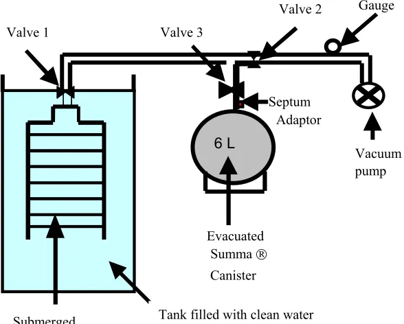
Figure 2. Diagram of experimental design for testing gas collection method

The experiment used water with dissolved oxygen concentrations lower than 10% saturation. The dissolved oxygen was removed by bubbling UHP helium gas through the water with a fine bubble diffuser (Point Four Systems Inc., model MBD 75, Richmond, BC, Canada) and Nalgene® vacuum tubing. The removal process of dissolved oxygen and dinitrogen by the helium bubbles was assumed to be the same, so the percent removal of dissolved oxygen and dinitrogen from saturated conditions should also be the same (Wold, 1973). In this experiment, the effect of dissolved N2 stripping would be minimal because of the low

dissolved dinitrogen concentrations in the water column. An accurate method should measure close to zero percent N2 if no air leaked into the system. However, the amount of N2

measured from the method would quantify the amount of N2 introduced into the system from

air contamination.

Gas Collector

Adaptor Septum

Vacuum pump

Evacuated Summa 

Canister

Gauge

Submerged

6 L

Valve 1

Valve 2 Valve 3

Water temperature was measured with a mercury thermometer and the atmospheric pressure was measured by a nearby weather station. Dissolved oxygen concentrations were measured with a Cole Parmer dissolved oxygen (DO) meter (WTW Multiparameter Kit, Vernon Hills, IL) and a galvanic DO probe (WTW Cellox 325, Cole Parmer Instrument Co, Vernon Hills, IL) before and after every experiment. The gas collector, with valve one open, was placed upright in the tank filled with water (fig. 2), and submerged until valve one rested on the surface of the water. Valve one was then closed to avoid any air contamination. Approximately 10 liters of UHP helium gas was bubbled directly under the submerged gas collector using Nalgene® tubing. No diffuser was used to distribute the helium into the water. To transfer gas from the gas collector to an evacuated (29.9 in. of Hg) SUMMA canister, both devices were connected with Nalgene® vacuum tubing and secured with Swaglok® hose clamps. Valve two was opened and the Precision Scientific high vacuum pump was used to evacuate the vacuum tubing to 29.9 in. of Hg. Valve two was closed before turning off the high vacuum pump. Valve one was opened and then valve three was slowly opened to allow the SUMMA canister to fill (approximately six liters). The gas collector was pushed down into the tank until valve one touched the surface of the water and then valves three and one were closed. This slightly pressurized the SUMMA canister and allowed gas samples to be taken from the septum-adapted nut with a syringe. A GASTIGHT Hamilton syringe (samplelockTM _{1005 SL, Sigma-Aldrich, Supelco Inc,}

2.3 Testing to Estimate a Volumetric Mass Transfer Coefficient

Standard procedures established by the American Society of Civil Engineers (ASCE, 1992) were incorporated with the method developed by Wilhelms and Martin (1992) to estimate a bubble volumetric mass transfer coefficient, [kLa]bubble, for determining the rate of dinitrogen

stripping. The procedures established by the American Society of Civil Engineers (ASCE, 1992) were used to estimate a total oxygen volumetric mass transfer coefficient for air bubbles in clean water. In addition to this, the approach developed by Wilhelms and Martin (1992) was used to determine the bubble and surface oxygen volumetric mass transfer coefficients from the total oxygen volumetric mass transfer coefficient. The total volumetric mass transfer coefficient would not be useful in determining the rate of stripping because it would include the surface gas exchange. It should also be noted that these procedures were written for evaluating oxygen mass transfer coefficients for diffuser aeration systems and not for dinitrogen stripping. However, assuming the ½ power relationship of diffusion coefficients in forced convection mass transfer, the [kLa] bubble value of dinitrogen gas would

be 94 % of that for oxygen gas (Cussler, 1997). Laboratory evaluations from Speece and Humenick (1973) also found the kL of N2 to be 89% of the kL of oxygen. Previous

researchers have used these ratios to model the mass transfer of dinitrogen and oxygen in aeration systems (Colt and Westers, 1982; DeMoyer et al., 2003). For this research, the ratio of 0.94 was used to estimate the dinitrogen value of [kLa] bubble from the laboratory

The experiment involved using a tank filled with 80 liters of clean water and a water column depth of 0.53 meters. Sodium sulfite and a cobalt catalyst were added to deoxygenate the water to 0.5 g m-3 of dissolved oxygen. The water was aerated with a fine bubble diffuser and every thirty seconds the dissolved oxygen was measured. Aeration continued until the water was fully saturated and in equilibrium with the atmosphere. Another experiment was done to determine the surface and bubble gas exchange. The water was deoxygenated again using sodium sulfate and a cobalt catalyst. UHP helium gas was bubbled through the water at the same gas flow rate as with the air pump. The dissolved oxygen was again measured every thirty seconds. The increase of dissolved oxygen in the water in this experiment was solely due to the oxygen absorbing at the surface. The helium was bubbled until the rate of oxygen stripped by the helium bubbles equaled the rate of oxygen absorbing at the surface and the dissolved oxygen concentration became constant. Water temperature was measured with a mercury thermometer before and after each experiment.

2.3.1 Calculations

The following equations from Wilhelms and Martin (1992) were used to determine the bubble and surface oxygen volumetric mass transfer coefficients from the total oxygen volumetric mass transfer coefficient. These equations assume that the hydrostatic pressure effects on the bubble are small and that the gas concentration inside the bubble did not change significantly. The gas transfer process that occurred while aerating with air bubbles over time can be broken into two parts: oxygen absorption at the water surface, and absorption from the air bubbles, which is described in equations 1, 2 and 3.

surface bubble t

C t

C dt

dC

   

∂ ∂ +    

∂ ∂

[

k_La

]

_surface(C_{s_atm} -C) t C surface =     ∂ ∂ (2)

[ ]

k_La _bubble(C_{s_bubble} -C)

t C bubble =     ∂ ∂ (3) where dt dC

= rate of total mass transfer per unit liquid volume, (g m-3 sec-1);

bubble t C     ∂ ∂

= rate of mass transfer through the surface of the bubble, (g m-3 sec-1);

surface t C     ∂ ∂

= rate of mass transfer through the water surface, (g m-3 sec-1);

[ ]

kLa_surface = liquid volumetric mass transfer coefficient for oxygen transfer at the

surface of the tank, (sec-1);

[ ]

kLa bubble = liquid volumetric mass transfer coefficient for oxygen transfer at the

surface of the bubble, (sec-1);

s

C = saturation concentration in equilibrium with a gas phase

atm

_ s

C = saturation concentration that is equilibrium with the atmospheric gas phase above the surface of the tank, (g m-3);

bubble

_ s

C = saturation concentration at the surface of the bubble that is assumed to be in equilibrium with the bulk gas phase, (g m-3);

C = the bulk solution concentration, (g m-3).

] ] [ exp[ ] ) ] [ ] ([ exp[ C - C C - C i s f

s _{k a k a t k a t}

total L surface

L bubble

L + = −

−

= (4)

The gas transfer process that occurred while bubbling helium gas can also be broken down into two parts: oxygen absorption at the water surface and oxygen being stripped from the water by the helium bubbles, which is described in equations 1, 2 and 5.

[ ]

k_La _bubbleC

t C bubble − =     ∂ ∂ (5)

The coefficients can be evaluated when equilibrium is reached and dC/dt equals zero. The equilibrium value, Ce, from the helium test is substituted for C in equations 5, 2 and 1. The

resulting proportion is shown.

[ ]

e atm s e bubble L surface L C C C a k a k − = _ ]

[ (6)

The equilibrium concentration, Ce, is the dissolved oxygen concentration when steady state

equilibrium occurs and the rate of stripped oxygen equals the rate of oxygen absorbed from the surface of the water. Equation 6 can be substituted into equation 4 to calculate the

surface La

k ]

[ and the [k_La]_bubblefrom the[k_La]_total. Once the [k_La]_bubble for oxygen is calculated, it is adjusted to a [k_La]_bubble for dinitrogen by multiplying by 0.94.

2.4 Field Implementation of Gas Collection Method

The third objective of this study was to design and demonstrate a simple and safe implementation of the gas collection method for measuring N2 gas emissions from an open

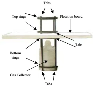
Figure 3. Device used to implement gas collection method

A nursery swine production unit located in Richlands, North Carolina, was selected as the site for implementing the gas collection method. The facility operated on a ‘pull-plug’ system with a cycle time of one week. After one week, the pits underneath the houses were emptied and the waste flowed by gravity into the lagoon treatment system (fig. 4). The lagoon treatment system was divided by hanging baffles to create a small anaerobic section and a partially aerated section (fig. 4).

Top rings

Gas Collector

Flotation board Tabs

Bottom rings

Tabs

Tabs Top rings

Gas Collector

Flotation board Tabs

Bottom rings

Tabs

Tabs Top rings

Gas Collector

Flotation board Tabs

Bottom rings

Tabs

Figure 4. Diagram of lagoon treatment system with dimensions. Arrows inside the lagoon represent the flow direction.

Waste entered the partially aerated section at the bottom of the hanging baffle that separated the two sections. The partially aerated section contained an InStreemTM Water Unit (IWU) and another hanging baffle. The IWU was designed and installed by Battelle Memorial Institute. The IWU provided mixing and dissolved oxygen by rotating nine 54 in. diameter discs that were submerged 21 inches into the water (see fig. D1 in appendix D). The disks

130 ft

170 ft

InStreemTM

Water Unit

Anaerobic Section Partially aerated _Section

Gas Collection device

Pipe from Swine Houses

Hanging Baffle

Figure 5. InStreemTM _{Water Unit installed in the lagoon treatment system}

The hanging baffle in this section was used to allow the water to flow in a circular direction as shown in figure 4. The gas collection device was used to measure N2 and methane

production in the partially aerated section of the lagoon treatment system (fig. 6).

Figure 6 . Picture showing InStreemTM _{Water Unit, gas collection device, and two hanging baffles}

weekly or biweekly depending on the length of time it took to fill the gas collector to at least 10 liters of gas. To transfer gas from the gas collector to an evacuated (29.9 in. of Hg) SUMMA canister, both devices were connected with Nalgene® vacuum tubing and secured with Swagelok® hose clamps. Valve two (fig. 1) was opened and two 12-volt DC powered vacuum pumps (miniature diaphragm twin pump 15D, Gast® Manufacturing Inc., Benton-Harbor, MI; diaphragm pump N85.3, KNF Neuberger Inc., Trenton, NJ) connected in series were used to evacuate the vacuum tubing to 28 in of Hg. The two DC powered vacuum pumps were powered by a Champion® motorcycle power sport battery (Agri-supply, Raleigh, NC). Valve two was closed before turning off the DC powered vacuum pumps. Valve one was opened and then valve three was slowly opened to allow the SUMMA canister to fill (approximately six liters). The gas collector was pushed down into the lagoon until valve one touched the surface of the water and then valves three and one were closed. The sample was then analyzed for dinitrogen and methane gas by GC. Gas analysis for each SUMMA canister were run in triplicate.

2.4.1 Calculations

T T L

La k a

k ₌ 20−

20 [ ]

]

[ θ (7) where

T La

k ]

[ = the volumetric mass transfer coefficient at some actual temperature, T (oC);

20

]

[k_La = the volumetric mass transfer coefficient at 20 o C.

Wastewater strength will also influence the mass transfer coefficient because of the presence of solids and surfactants (Baker, et al., 1975; Mihelcic et al., 1993). The mass transfer coefficient is corrected by using an alpha factor (equation 8).

r clean wate L water process L a] [k a] [k =

α (8)

Previous researchers have reported alpha values for different types of aeration devices and various wastewater strengths (Bass and Shell, 1977; Hwang and Stenstrom, 1985; Stenstrom and Gilbert, 1981; U.S. EPA, 1989). Values of alpha for oxygen have been reported to range from 0.4 to 0.9 in fine-bubble diffusers systems with mixed liquor domestic wastewater (Hwang and Stenstrom, 1985). The alpha values were found to increase with increasing treatment. Alpha factors also decreased with increasing airflow rate and increasing mixed liquor depth. The alpha factors ranged from 0.6 to 0.9 at a mixed liquor depth of 1.5 m, which would be similar to a lagoon treatment system. Other researchers have reported that alpha values of oxygen decreased from 0.9 to 0.4 when the total solids concentration of poultry waste increased from 1% to 5.5% in an oxidation ditch using cage rotors (Baker et al., 1975). After looking at the trends of previous research and assuming that the ratio of kLa

for oxygen and dinitrogen are unaffected by wastewater strength, so that the same α value would apply, a range of alpha values of 0.6 to 0.8 were selected to correct the kLa for process

The rate of gas production will also influence kLa values because at a higher gas flow rate

more bubbles will be produced and therefore increase the interfacial area available for transfer. If the same bubble size and rise velocity occurs in both the field and the lab, the relationship of gas flow rates to the total specific areas and volumetric mass coefficients can be described using equation 9 (see appendix E-3 for calculation).

lab L field L lab field lab field a k a k a a Q Q ] [ ] [ =

= (9)

where

Q_field = gas production rate in a lagoon treatment system (m3 sec-1);

Q_lab = average gas flow rate used in experiment 2 (m3 sec-1);

field

a = total specific area (At/V) in field conditions (m2 m-3); a_lab = total specific area (At/V) in lab conditions (m2 m-3);

At = total bubble surface area (m2); V = total liquid volume (m3).

While it is difficult to calculate total specific areas, a ratio of the gas production rate in an open pond treatment system to the average gas flow rate in the laboratory can be used to estimate the field volumetric mass transfer coefficient from the laboratory volumetric mass transfer coefficient. The dinitrogen bulk solution concentration, C, was estimated using an air solubility concentration table developed by Colt (1984) with the appropriate liquid field temperature and salinity value of 5 ppt. The dinitrogen concentration at the surface of the bubbles, Cs_bubble, was estimated by using Henry’s law. The adjusted volumetric mass

transfer coefficient, C and Cs_bubble were used to estimate the rate of dinitrogen stripped per

3.0 RESULTS AND DICUSSION

3.1 Gas Chromatography

The gas chromatography testing revealed relatively little N2 contamination. System blanks

and blank injections measured 0.038 and 0.095 % N2, respectively (Table 1). The standard

deviation was higher than the average percent N2 for the system blanks and blank injection.

The coefficient of variation for this instrument at its detection limits would be close to 100%. These results reveal the instrument is at its detection limit for the blank and blank injection. The percent recoveries from calibration gases were 101% for 10% N2, 100% for 30% N2, and

98.4 % for 50% N2. This indicates that the instrument calibration remained stable during

measurement periods.

Table 1. Testing gas chromatography method[a]

Sample Percentage of N2

Average

Percentage of N2

Standard Deviation Number of observations

System Blank [b] _{0.038 0.068 15}

Blank injection [c] _{0.095 0.105 15}

10% N2 / 80 % CH4 [d] 10.1 0.36 15

30% N2 / 50 % CH4 [d] 30.0 0.52 15

50% N2 / 4 % CH4[d] 49.2 1.20 15

[a] _{Testing to determine background N}

2 and GC accuracy [b] _{Purge sample loop and injection port with helium}

[c] _{Penetrate septum with syringe needle with no sample injection} [d] _{Standard gases}

3.2 Gas Collection Method Testing

contamination associated with the sampling procedure. This value is consistent with the calculated detection limit for determining N2 by using the standard deviation of the blank

injection (Table 1) and adopting the standard convention that the detection limit is equal to 3 times the standard deviation plus the blank (3 x 0.105 % + 0.095% = 0.41%) when the number of observations is 8 or greater.

Table 2. Experiment 1: Results from testing gas collection method with initial low dissolved oxygen and dinitrogen concentrations for air contamination

Dissolved Oxygen (g m-3₎

Average (std)

Dissolved N2 and O2 % Saturation

Average (std)

% N2 Gas Measured from Collection Method

Average (std)

Number of observations[a]

0.80 (0.11) 9.4 (1.2) 0.57 (0.097) 8

[a] _{Gas samples were analyzed in triplicate.}

3.3 Estimation of Mass Transfer Coefficient

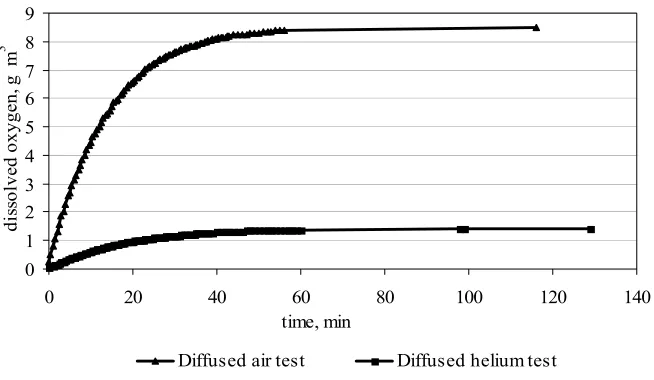
This experiment involved bubbling air to oxygenate the water column from 0.5 g m-3 to an average saturation concentration, Cs_atm of 8.58 g m-3. This part of the experiment was

replicated three times. The dissolved oxygen concentrations measured over time for the last replication are shown in figure 7. This experiment also involved bubbling helium gas through the water column. For this part the initial dissolved oxygen concentration was also 0.5 g m-3 and the finial equilibrium dissolved oxygen concentration, Ce, was 1.43 g m-3. The

0 1 2 3 4 5 6 7 8 9

0 20 40 60 80 100 120 140

time, min

dis

so

lv

ed

oxyge

n,

g m

3

Diffused air test Diffused helium test

Figure 7. Dissolved oxygen measurements for diffused air and diffused helium in a tank filled with clean water.

A total volumetric mass transfer for oxygen was estimated using SAS® (2001), statistical software, with the nonlinear regression model described in ASCE (1992) and the dissolved oxygen measurements for the experiments using diffused air. The average total volumetric mass transfer coefficient, [kLa]total was calculated to be - 4.13 hr-1 with a water temperature of

24.3 degrees Celsius. The average gas flow rate when bubbling helium and air was 2.0 liters min-1. Equations 4 and 6 and the values for Ce and Cs_atm, were used to calculate [kLa]bubble

from the [kLa]total. This coefficient for oxygen was then adjusted by multiplying by the ratio

3.4 Field Implementation of Gas Collection Method

Preliminary field data are reported to demonstrate the use of this method and the potential importance of N2 stripping. The adjusted volumetric mass transfer coefficient, C and Cs_bubble

were used to estimate the rate of dinitrogen stripped per unit liquid volume using equation 3. The liquid depth was multiplied by this rate to determine the rate of dinitrogen stripped per unit of surface area under the gas collector. The error associated with atmospheric contamination (0.57% N2) found in the first experiment was subtracted from the total percent

N2 measured with the gas collection method. The rate of stripped N2 was subtracted from the

total rate of N2 measured to estimate the rate of biologically produced N2. An average alpha

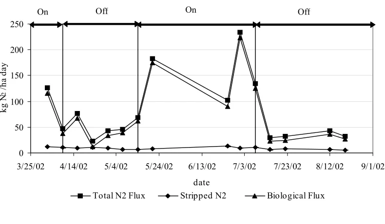
value of 0.7 was used to estimate the dinitrogen volumetric mass transfer coefficient, which was used to calculate these rates during periods when the rotating disk aerator was off and on (fig. 8).

Figure 8. Dinitrogen flux measurements and stripping estimations using an alpha value of 0.7. Graph labeled when rotating disk aerator was on and off.

0 50 100 150 200 250

3/25/02 4/14/02 5/4/02 5/24/02 6/13/02 7/3/02 7/23/02 8/12/02 9/1/02 date

kg N

2

/ha

da

y

Total N2 Flux Stripped N2 Biological Flux Series4 Series5 Series6

Off

Off On

The total N2 gas flux was significantly higher during the periods when the rotating disk

aerator was on than when the aerator was off (p = 0.0020). However, the estimates of the flux due to stripping remained low regardless of the aeration status. The estimates of nitrogen flux due to biological activity, total flux minus flux due to stripping, were statistically different from zero when aeration was on and when aeration was off. When aeration was on, the average flux due to stripping was 10.5 kg N2 ha-1d-1 out of a total

average flux of 161 kg N2 ha-1d-1, or 6.5% of the total nitrogen flux. However, when the

aeration system was off, the average flux of stripped dinitrogen was 7.86 kg N2 ha-1d-1 out of

a total flux of 40.45 kg N2 ha-1d-1, or 19.4% of the total nitrogen flux. The data suggest that

the consideration of the effect of gas stripping on nitrogen emissions may be quite significant.

Bubble size is an important component of the calculation of flux due to gas stripping because the ratio of surface area to volume is proportional to the reciprocal of the bubble diameter. For a given volume of gas production, total surface area will double if bubble diameter is reduced by half. A larger total surface area would enable more mass transfer to occur from the liquid to the bubbles, increasing the flux of stripped nitrogen. For example, if the bubble diameter with aeration on is half of that estimated in this work, the stripped nitrogen flux would double to 21 kg N2 ha-1d-1 or 13% of the total flux. With aeration off, the stripped flux

would be 15.7 kg N2 ha-1d-1 or 38.8% of the total flux. Because of the potential for

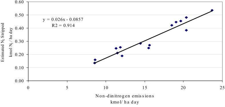
A positive linear relationship was found between the non-dinitrogen flux and the estimated stripped N2 flux (fig. 9). The calculation method assumed that the transfer coefficient, kLa,

was proportional to total gas flow. However, the relationship of stripped N2 flux to total gas

flux was not as good as that to non-dinitrogen flux because the transfer rate also depends on the concentration of N2 inside the gas bubble. Based on the trend in figure 9, an open

treatment system with a higher methane production may strip dissolved dinitrogen at higher rate until a dynamic equilibrium is established between dinitrogen leaving the system by stripping and dinitrogen entering the system from the atmosphere.

Figure 9. Relationship between estimated stripped N2 flux when using an alpha value of 0.7 with measured

non-dinitrogen flux.

Ammonia loss from animal waste systems is an important environmental concern. In order to properly implement abatement strategies, accurate estimates of the form and flux of nitrogen are needed. The method described above represents another tool to actually

measure a form of nitrogen that is very difficult to measure and that has often been ignored. The method uses engineering procedures to address important complicating factors in the

y = 0.026x - 0.0857 R2 = 0.914

0.00 0.10 0.20 0.30 0.40 0.50 0.60

0 5 10 15 20 25

N o n -d in itro g e n emis s io n s kmo l/ h a d ay

Es

tim

at

ed

N2

St

ri

pp

ed

kmo

l N

2

/ h

a d

measurement of N2 emissions from open pond systems. The application of this method will

4.0 CONCLUSIONS

The developed gas collection method for measuring dinitrogen gas emissions from lagoon treatment systems was critically tested in a laboratory to ensure reliable dinitrogen gas measurements. The results from laboratory testing revealed that dinitrogen can be measured with low amounts of dinitrogen atmospheric contamination (0.57% N2) when the method is

done properly and when the equipment is functioning like it should. I found it is crucial to leak check the SUMMA canisters prior to sampling and that the sealant on carboy lids be carefully monitored. The sealant on the carboy can be easily checked by filling the carboy with air, submerging it underwater and then checking for bubbles. If the lid is not properly sealed air bubbles will develop within a couple of seconds. This equipment needs close monitoring because any air leakage will give wrong measurements. The results from the gas chromatography testing revealed that the instrument was running in excellent condition and there was very little atmospheric N2 in blanks (0.038% N2), blank injections (0.105% N2) and

analysis of standard gases.

as much as 39% of the total N2 loss. This is significant and should be considered when

measuring for biological denitrification.

The results from implementing the method on a partially aerated swine waste treatment system suggested that N2 was biologically produced from microbial denitrification at a rate

higher than could be produced from stripping dissolved N2. The total measured dinitrogen

was also found to be significantly higher when aeration was on (p=0.0020) and was on average 161 kg N2 ha-1day-1. When the aeration was off the average total measured

dinitrogen flux was 40.4 kg N2 ha-1day-1. Harper and Sharper (1998) reported dinitrogen

emissions of 120.1 to 8.9 kg N2 ha-1 day-1 for two anaerobic lagoons in North Carolina. The

results from this study are higher than the dinitrogen emissions reported by Harper and Sharpe; however, this would be expected because the lagoon treatment system in this study was partially aerated and had more opportunity for microbial nitrification and denitrification. Harper and Sharpe also did not consider stripped dinitrogen to be apart of their flux measurements. The actual nitrogen loss from denitrification could be 20% to 40% less than what they have reported.

R

EFERENCES

Aneja, V.P., B. Bunton, J.T. Walker, and B.P. Malik. (2001). Measurement and analysis of atmospheric ammonia emissions from anaerobic lagoons. Atmospheric Environment. 35: 1949-1958.

ASCE. (1992). Measurement of oxygen transfer in clean water. 2nd ed. New York, NY.: ASCE.

Baker, D. R, R. C. Loehr, and A. C. Anthonisen. (1975). Oxygen Transfer at High Solids Concentrations. Journal the Environmental Engineering Division, Proceeding of the

American Society of Civil Engineers. 101: 759-774.

Bass, S. J. and G. L. Shell. (1977). Evaluation of Oxygen Transfer Coefficients of Complex Wastewaters. In Proceedings of the 32nd Industrial Waste Conference. 953-967. Ann Arbor, Mic.: Ann Arbor Science.

Bock, E., I. Schmidt, R. Stuven and D. Zart. (1995). Nitrogen loss caused by denitrifying

Nitrosomonas cells using ammonium or hydrogen as electron donor and nitrite as the

electron acceptor. Archives of Microbiology. 163: 16-20.

Bouck, G. R. (1982). Gasometer: An inexpensive device for continuous monitoring of dissolved gases and supersaturation. Transactions of the American Fisheries Society. 111: 505-516.

Clesceri, L. S., A. E. Greenberg & R. R. Trussel. (1995). Standard Methods for the

Examination of Water and Wastewater.19 ed. 2810: Dissolved gas supersaturation

.APHA, AWWA, WPCF.

Crites, R., and G. Tchobanoglous. (1998). Small and Decentralized Wastewater

Management Systems. Boston: McGraw-Hill.

Colt, J., and H. Westers. (1982). Production of gas supersaturation by aeration.

Transactions of the American Fisheries Society. 111: 342-360.

Colt, J. (1984). Computation of Dissolved Gas Concentrations in Water as Functions of

Temperature, Salinity, and Pressure. Bethesda, Maryland: American Fisheries

Cussler E.L. (1997). Diffusion: Mass transfer in fluid systems, 2nd _{ed., Cambridge:}

Cambridge University Press.

DeMoyer, C. D., E. L. Schierholz, J.S. Gulliver, and S. C. Wilhelms. (2003). Impact of bubble and free surface oxygen transfer on diffused aeration systems. Water

Research. 37: 1890-1904.

Goreau, T.J., W. A. Kaplan, S. C. Wofsy, M. B. McElroy, F. W. Valois and S. Watson. (1980). Production of NO-2 and N2O by nitrifying bacteria at reduced concentrations

of oxygen. Applied and Environmental Microbiology. 40(2): 526-532.

Harper, L. A. and R. R. Sharpe. (1998). Ammonia emissions from swine waste lagoons in the southeastern U. S. coastal plains. USDA-ARS Agreement No. 58-6612-7M-022. Raleigh, NC.: North Carolina Dept. of Environmental and Natural Resources. Harvey, H. H. (1975). Gas disease in fishes- a review. In Chemistry and Physics of Aqueous

Gas Solutions, 450-485. Princeton, New Jersey.: The Electrochemical Society.

Hwang, H. J. and M. K. Stenstrom. (1985). Evaluation of fine-bubble alpha factors in near full-scale equipment. Journal of the Water Pollution Control Federation. 57(12): 1142-1151.

Jetten, M. S. M., M. Strous, K. T. van de Pas-Schoonen, J. Schalk, U. G .J. M. van Dongen, A. A. van de Graaf, S. Logemann, G. Muyzer, M. C. M. van Loosdrecht and J.G. Kuenen. (1999). The anaerobic oxidation of ammonia. FEMS Microbiology Reviews. 22: 421-437.

Jones, M. L., S. K. Liehr, J. J. Classen and W. Robarge. (2000). Mechanisms of dinitrogen gas formation in anaerobic lagoons. Advances in Environmental Research. 4: 133-139.

Koelliker, J. K. and J. R. Miner. (1973). Desorption of ammonia from anaerobic lagoons.

Transactions of the ASAE. 16 (1): 148-151.

Mc Neil, C. L., B. D. Johnson, and D. M. Farmer. (1995). In-situ measurement of dissolved nitrogen and oxygen in the ocean. Deep-Sea Research I. 42 (5): 819-826.

Mihelcic, J. R., C. R. Baillod and J. C. Crittenden. (1993). Estimation of VOC emissions from wastewater facilities by volatilization and stripping. Journal of Air and Waste Association. 43: 97-105.

Mulder, A., A. A. van de Graaf, L. A. Roberston and J. G. Kuenen. (1995). Anaerobic ammonium oxidation discovered in a denitrifying fluidized bed reactor. FEMS

Microbiology Ecology. 16: 177-184.

Phillips, J. (1995). Control and pollution prevention options for ammonia emissions. EPA Contract No. EPA-456/R-95-002. Research Triangle Park, NC.: U.S. Environmental Protection Agency.

Poth, M. (1986). Dinitrogen production from nitrite by Nitrosomonas isolate. Applied and

Environmental Microbiology. 52 (4): 957-959.

SAS. (2001). SAS User’s Guide: Statistics. Ver. 8.2. Cary, NC.: SAS Institute, Inc. Schmidt, I. and E. Bock. (1997). Anaerobic ammonia oxidation with nitrogen dioxide by

Nitrosomonas eutropha. Archives of Microbiology. 167: 106-111.

Speece R. E., and M. J. Humenick. (1973). Carbon dioxide stripping from oxygen activated sludge systems. Journal of Water Pollution Control Federation. 45 (3): 412-423 Stenstrom, M. K., and R. G Gilbert. (1981). Effects of alpha, beta, and theta factor upon the

design, specification and operation of aeration systems. Water Research. 15: 643-654.

Swinnerton, J. W., V. J. Linnenbom, C. H. Cheek. (1962). Determination of dissolved gases in aqueous solutions by gas chromatography. Analytical Chemistry. 34(4): 483-485. Tchobanoglous, G. and F. Burton. (1991). Wastewater Engineering. New York, NY.:

McGraw-Hill.

U.S. EPA. (1989). Design Manual: Fine Pore Aeration Systems. EPA Contract No. EPA-625/1-89-023. Cincinnati,OH.: EPA. Center for Environmental Research and Development.

Walker, J. T., V. P. Aneja, and D. A. Dickey. (2000). Atmospheric transport and wet deposition of ammonium in North Carolina. Atmospheric Environment. 34: 3407-3418.

Weiss, R. F. (1970). The solubility of nitrogen, oxygen, and argon in water and seawater.

Deep Sea Research. 17: 721-735.

Wilhelms, S. C. and S.K. Martin. (1992). Gas transfer in diffused bubble plumes. In

Jennings SM and Bhowmilk NG, Eds. Hydraulic Engineering: saving a threatened

resource-in search of solutions, 317-322. New York, NY.: ASCE.

Table A1. Materials used to make the SUMMA® can devices used in this research

Part Name Part Number Company or person End connection or description Cost $

Adjustable Hose

Clamps MS-HCC-8

Swagelok® Raleigh

Valve and Fitting Co. ½ in. OD hoses 1.90 Automatic tube Weld

(ATW) Reducing Union

316-6-ATW-6-4 _{Valve and Fitting Co.} Swagelok® Raleigh

3/8 in. OD tube stub at one end and ¼ in. OD tube stub at

the other.

13.60

Crawford Special

Adaptor SS-404-1-0001

Swagelok® Raleigh Valve and Fitting Co.

A ¼ in. nut adapted to fit a

septum inside 7.20

DL series diaphragm valve (valve 3)

SS-DLS-4 _{Valve and Fitting Co.} Swagelok® Raleigh ¼ in. tube fitting on both ends 144.70

Female branch tee: _{SS-400-3-4TTF} Swagelok® Raleigh Valve and Fitting Co.

Identical tube stubs with ID = ¼ in. and female pipe with ¼

in. opening

23.70

Front and Back Ferrule SS-403-1 _{SS-404-1 Valve and Fitting Co.} Swagelok® Raleigh ¼ in. OD 0.73 _0.65

Hose connector (1) SS-4-HC-A-401 _{Valve and Fitting Co.} Swagelok® Raleigh ¼ in. ID hose connector and _{¼ in. tube adapter} 7.20

Hose connector (2) SS-4-HC-7-4 _{Valve and Fitting Co.} Swagelok® Raleigh

¼ in. ID hose connector and ¼ in. female NPT taper thread

end

10.80

Nut SS-402-1 _{Valve and Fitting Co.} Swagelok® Raleigh ¼ in. OD 1.40 Plug valve

(valve 2) SS-4P4T2

Swagelok® Raleigh Valve and Fitting Co.

¼ in. male American standard pipe thread (NPT) on both

ends

36.50

Reducer SS-400-R-6 _{Valve and Fitting Co.} Swagelok® Raleigh

¼ in. OD tube stub on one end and 3/8 in. OD on the

other end

6.70

Septums ₂₀₄₂₁ Sigma-Aldrich _{Supelco Inc.} gr-2 gray, 11mm

33.50 for one pack of 100

septums Stainless seal kit for

DL valve SS-3DK-DS

Swagelok® Raleigh

Valve and Fitting Co. NA 5.50

SUMMA® canister NA Bob Seila Top connection was a 3/8 in. _{OD union tee} free

Table A2. Materials used for the carboy device, not including the flotation device

Part Name Part Number _Company Supply End connection or _{description/size} Cost $

Hose connector (1) SS-4-HC-A-401 _{Valve and Fitting Co.} Swagelok® Raleigh ¼ in. ID hose connector and _{¼ in. tube adapter} 7.20

Nalgene® Polycarbonate

ClearboyTM _{Carboy 16101-186} VWR Scientific

Products 21 Liter volume 326.68 for four

Nut (fastener) NA BAE research shop ¼ in. Free

Outdoor Goop® NA Lowes® NA 4.87

Plug Valve (1) SS-4P4T _{Valve and Fitting Co.} Swagelok® Raleigh ¼ in. OD tube fittings both _ends 42.00

Rubber washers NA Lowes® 7/16 by 1 by 1/16 in. 0.62 for two

Stainless Steel Bulk head

reducer SS-400-R1-4

Swagelok® Raleigh Valve and Fitting Co.

¼ in.OD tube stub connection on one end and ¼

in. tube fitting

10.40

silicone sealant NA Lowes® NA 2.86

Table A3. Materials used for flotation device

Part Name and

description Dimensions Company Number per system Cost $

¼ in. thick, 1 in. wide aluminum: used for the

tabs and side bars

Tabs: 2 in. long Short bar: 10 in. long Long bar: 20 in. long Total length: 14 ft per device

NCSU Research Shop

16 tabs 4 short bars,

4 long bars 1/8 in. thick, 1 in. wide

aluminum: used for the rings

13 in. diameter rings: 40.8 in. length aluminum

piece

NCSU Research

Shop 4 rings

Blueboard Styrofoam 2 in. by 4 ft. by 8 ft Hughes Supply. _Inc. 2 20.00

Fiber glass boards Lowes 1 25.00

galvanized bolts ¼ in. 4 ½ long Lowes 4 0.33 each

galvanized bolts ¼ in. 3 ½ long Lowes 8 0.29 each

galvanized nuts ¼ in Lowes 12 0.07 each

RustoelTM _{Spray Paint NA Burke Brothers 1 4.23}

stainless steel wing nuts ¼ in NCSU Research _Shop 4 free

Table A4 . Other material / equipment that are not shown in tables A1, A2, and A3.

Part Name:

description/model number Part or catalog number

Supply

Company Dimensions or capacity Cost $ Hamilton samplelockTM

syringe: 1005 SL 26286

Sigma-Aldrich

Supleco Inc. 5-ml, 22 gauge 76.40

Belt Drive AC Powered Vacuum Pump:

Model D 150

5122005 Precision Scientific

29.9 in. Hg max. vacuum, 150 LPM open

flow

Borrowed from Roberto Munello

High Vacuum DC 12-volt

powered pump: N85.3 DC NA KNF Neuberger Inc.

29.2 in. Hg max. vacuum, 5.5 LPM open

flow 364.55

Nalgene® Vacuum tubing:

PVC 180 14 176 6B Fisher Scientific

¼ in. ID, 3/16 in wall

thickness 32.69 for one box (10ft) High Vacuuum DC 12

volt powered pump: 15D

5150 NA

Gast® Manufacturing

Inc. 25 in. Hg max. vacuum, 6 LPM open flow ? Ashcroft® Industrial

vacuum gauge 2C569 Grainger®

Max vacuum 30 inch

Hg 46.95

16 in. tool box with metal

latches NA Lowes NA 7.96

Champion® DC Motorcycle power sport

battery (12 volt)

Table A5. Supply company information

Company Name Address City, State, zip code Phone number

Agri Supply® 409 Highway 70 East Garner, NC, 27529 1-919-772-0865 Burke Brothers 5227 Hillsborough St. Raleigh, NC, 27606 1-919-851-1211 Cole Parmer Instrument Co. 625 East Bunker Court. Vernon Hills, IL, 60061-1844 1-800-323-4340

Fisher Scientific NA Atlantic, GA

Gast® Manufacturing Inc. 2300 Highway M-139 Benton Harbor, MI, 49022 1-616-926-6171 Grainger® 4820 Signett Drive Raleigh, NC, 27604 1 -919-790-0888 Hughes Supply. Inc. 2111 New Hope Church _Rd. Raleigh, NC, 27604 1-919-872-6543 KNF Neuberger Inc. Two Black Forest Road Trenton, NJ, 08691-1810 1-609-890-8600

Lowes 1575 US HWY 70 West Garner, NC, 27529

National Specialty Gases P.O Box 12013 Research Triangle Park, NC, ₂₇₇₀₉ 1-919-544-3772 National Welders Supply Co. 4301 Capital Blvd. Raleigh, NC, 27604-3497 1-919-876-6710

Point Four System, Inc. 100-13720 Mayfield Place Richmond, BC, Canada, V6V _2EA 1-800-267-9936

Precision Scientific 170 Marcel Dr. Winchester, VA, 22602 1 -800- 621-8820

Shimadzu Scientific Instruments, Inc. 3070 Business Park Drive, _{Suite H,} Norcross, GA, 30071 1-800-951-9167

Supelco Inc. Bellefonte, PA, 16823 1-800-247-6628

Swagelok® Raleigh Valve and Fitting

Co. 2621 Rowland Road Raleigh, NC 1-919-878-8085

VWR Scientific Products, VWR

B-1 Procedure used to build the SUMMA® Canister devices

The SUMMA canisters® were donated from Bob Seila and were already mounted with a (3/8 in. OD) union tee. The following is a step by step procedure used to build the SUMMA ® canister devices.

1) Weld the side bend of the union tee to the 3/8 in. OD tube stub end of the reducer (SS-400-R-6).

2) Weld the top bend of the union tee to the 3/8 in. OD end of the automatic tube weld (ATW) reducing union (316-6-ATW-6-4).

3) Remove the seals and other components found inside the diaphragm valve

(SS-DLS-4). Follow the Swagelok® procedures found in stainless steal replacement kit for the DL valve (SS-3DK-DS).

4) Weld the top of the ATW reducing union (¼ in. OD) to the bottom tube stub connection (¼ in. OD) of the diaphragm valve (SS-DLS-4).

5) Weld a (¼ inch OD) stainless tube pipe, about 1 inch in length, to the top tube stub connection of the diaphragm valve.

6) Attach a ¼ in. OD nut (SS-402-1) using both the front (SS-403-1) and back (SS-404-1) ferrules to the ¼ in. OD tube pipe. For detailed directions for this contact your Swagelok® supplier.

7) Tightly screw the female branch tee (SS-400-3-4TTF) inside the 1/4 in. OD nut from one of the ¼ tube stub connections of the tee.

8) Wrap teflon® tape around the ¼ in. NPT thread connection of the plug valve (valve 2,

9) Wrap teflon® tape around the other ¼ in. NPT thread connection of the plug valve.

Tightly scew the ¼ in. male connection of the plug valve inside the 1/4 in. female connection of the hose connector 2 (SS-4-HC-7-4).

10) Attach a ¼ in. OD nut (SS-402-1) using both the front (SS-403-1) and back (SS-404-1) ferrules to the ¼ in. OD tube pipe connection of the hose connector 1 (SS-4-HC-A-401).

11)Tightly screw this piece on the other ¼ in. tube stub connection of the female branch tee (SS-400-3-4TTF)

12)Since the old seals were removed from the diaphragm, new ones must be put back in. Replace the news seals using the stainless steel replacement kit for the DL valve (SS-3DK-DS).

B-2Procedure to assembly carboy lid, fittings and plug valve

1) Cut a 3/8 in. diameter hole in the center of the carboy lid. Use sand paper to roughen both the top and inside surface around the hole.

2) Place one rubber washer through the ¼ in. OD tube stub end of the stainless steel bulk head reducer (SS-400-R1-4). Having the tube stub end down, place stainless steel bulk head reducer through the hole in the center of the carboy lid.

3) Place another rubber washer through the end of the ¼ in. OD inside the lid. Tightly fasten with a stainless steel ¼ in. nut.

4) Remove the ¼ in. nut from the tube fitting end of the stainless steel bulk head reducer and attach the bottom tube fitting connection of the plug valve (1) (SS-4P4T).

5) Attach the ¼ in. OD nut (SS-402-1) with the ¼ in. tube connection of the hose connector 1 (SS-4-HC-A-401) and reattach to the top connection of the plug valve. 6) Generously apply the Outdoor Goop® around the base of the stainless steel bulk head

B-3 Procedure to build flotation device

Aluminum frame: See Appendix F, for the drawings of the frame:

1) Cut the 1/8 in. thick, 1 in. wide aluminum into 4 pieces that are 41 inches long. Bend the aluminum pieces to make a circle and weld the two ends together. This will make 4 (13 in. diameter) rings.

2) Cut the ¼ in. thick, 1 in. wide aluminum to make 16 (2 in. long) tabs. Continue to cut the ¼ in. thick aluminum into 4 long bars (20 in. long) and 4 short bars (10 in. long). 3) Weld the tabs to each end of the bars. The top and bottom tabs will be positioned in

the opposite direction (fig. B1). The short bars will make the top piece and the longer bars will make the bottom piece.

Figure B1. Diagram of aluminum bars and tabs used to build the flotation device

(not drawn to scale)

short (10 in. length) bar that will attach to the rings 2 in. long tab that will keep the carboy inside the frame

2 in. long tab that will attach to the

flotation device

4) Weld the four short (top piece) bars inside two rings and the four longer bars inside the other two rings. When doing this, it is crucial to align the one bottom bar with a particular top bar because they will be bolted together. Mark each set (one top and one bottom) so you can remember when you do bolt them together. See the drawings for a diagram. For the tabs that will be used to bolt the flotation device, drill a ¼ in. diameter hole in the center of the tab. It is again very crucial to align the pairs together when doing this.

Building the flotation board

1) Cut the styrofoam blue board into one 30 in. by 48 in. (0.76 m by 1.2 m) rectangle. Cut two 30 in. by 48 in. (0.76 m by 1.2 m) rectangles with the fiber glass board. 2) Cut a 13 in. (330 mm) diameter circle in the middle of all three boards, making sure

all three boards have the circle in the same place. Cut a square notch (76 mm by 76 mm) on one edge of the circle with all three boards.

3) Drill eight (¼ in. diameter) holes along the edge of all the boards and 4 (¼ in.

Figure B2. Diagram to show the top view of flotation device and the nuts and bolts locations.

Diagram is not drawn to scale.

Figure B3. Diagram of styrofoam and fiberglass boards bolted together. Diagram is not drawn to scale.

Nut

Styrofoam board

The head of the bolt Fiberglass board

washer washer

Nut and bolt Wingnut

Table C1. Dinitrogen and methane emissions from the lagoon treatment system

%N2 -

0.57%N2 % CH4 Pressure Temp Carboy

Volume Time

total Carboy

N2 Gas emission

CH4 Gas emissions

Date

Collected atm K Liters days mols kg N(ha*d) 2/ kg CH(ha*d) 4 /

4/2/02 16.07 73.43 1.00 293 20 5 0.835 127 332

4/9/02 7.93 81.73 1.01 293 21 7 0.886 47.4 280

4/16/02 12.82 71.82 1.01 293 21 7 0.881 76.2 244

4/23/02 3.81 80.46 1.00 293 21 7 0.878 22.6 273

4/30/02 7.47 78.24 1.00 293 20.5 7 0.855 43.1 258

5/7/02 12.53 75.70 1.01 297 13 7 0.537 45.4 157

5/14/02 17.00 70.24 1.00 297 14.5 7 0.594 68.1 161

5/21/02 31.05 58.66 1.01 297 21 7 0.870 182 197

6/25/02 15.24 79.17 1.01 301 21 6 0.855 103 305

7/1/02 34.97 58.75 1.01 304 21 6 0.847 233 224

7/8/02 23.53 67.80 1.01 304 21 7 0.849 135 222

7/15/02 10.71 82.29 1.00 304 10 7 0.401 29.0 128

7/22/02 9.17 82.55 1.00 304 13 7 0.524 32.4 167

8/12/02 11.27 77.18 1.00 303 20 10 0.808 43.0 169

Table C2. Estimations of the stripped dinitrogen from field data and using an alpha valve of 0.7. Cs C _Volume Carboy Time _Flowrate Gas _{20 oC temp} (Field Ka) Field Ka field _temp Lagoon N2 in

carboy

rate of stripped N2

Date Collected g/m3 g/m3 Liters days m3/hr 1/hr 1/hr mol g/(m^3 hr)

4/2/02 3.02 14.67 20 5 1.667E-04 -2.85E-03 -2.81E-03 0.134 0.0328

4/9/02 1.49 14.67 21 7 1.250E-04 -2.14E-03 -2.11E-03 0.070 0.0278

4/16/02 2.41 14.67 21 7 1.250E-04 -2.14E-03 -2.11E-03 0.113 0.0259

4/23/02 0.72 14.67 21 7 1.250E-04 -2.14E-03 -2.11E-03 0.033 0.0294

4/30/02 1.40 14.67 20.5 7 1.220E-04 -2.08E-03 -2.06E-03 0.064 0.0273

5/7/02 2.20 13.67 13 7 7.738E-05 -1.32E-03 -1.44E-03 0.067 0.0165

5/14/02 2.98 13.67 14.5 7 8.631E-05 -1.47E-03 -1.61E-03 0.101 0.0172

5/21/02 5.44 13.67 21 7 1.250E-04 -2.14E-03 -2.33E-03 0.270 0.0191

6/25/02 2.46 12.6 21 6 1.458E-04 -2.49E-03 -3.02E-03 0.130 0.0306

7/1/02 5.47 12.21 21 6 1.458E-04 -2.49E-03 -3.23E-03 0.296 0.0217

7/8/02 3.68 12.21 21 7 1.250E-04 -2.14E-03 -2.77E-03 0.200 0.0236

7/15/02 1.68 12.21 10 7 5.952E-05 -1.02E-03 -1.32E-03 0.043 0.0139

7/22/02 1.44 12.21 13 7 7.738E-05 -1.32E-03 -1.71E-03 0.048 0.0184

8/12/02 1.79 12.4 20 10 8.333E-05 -1.42E-03 -1.80E-03 0.091 0.0191

8/19/02 1.87 12.4 10 7 5.952E-05 -1.02E-03 -1.29E-03 0.047 0.0135

Table C3. The estimated rate of stripping and biological emissions (using an alpha value of 0.7).

rate of stripped N2

actual Liquid depth

Rate of

Stripped N2 Biological N2

Total Gas emissions

Non-Nitrogen emissions Date

Collected g/(m^3 hr) m kmol N(ha day) 2 / kmol N2 / (ha day) total kmol / (ha day) total kmol / (ha day)

4/2/02 0.03277 1.52 0.427 3.99 28.18 23.65

4/9/02 0.02781 1.52 0.362 1.24 21.35 19.66

4/16/02 0.02587 1.52 0.337 2.30 21.22 18.50

4/23/02 0.02945 1.52 0.383 0.33 21.16 20.35

4/30/02 0.02733 1.52 0.356 1.09 20.60 19.06

5/7/02 0.01652 1.68 0.238 1.38 12.93 11.31

5/14/02 0.01717 1.68 0.247 2.18 14.31 11.88

5/21/02 0.01914 1.68 0.275 6.22 20.96 14.45

6/25/02 0.03061 1.75 0.459 3.28 24.02 20.36

7/1/02 0.02173 1.83 0.341 8.07 23.80 15.48

7/8/02 0.02358 1.83 0.370 4.54 20.45 15.64

7/15/02 0.01387 1.83 0.217 0.88 9.66 8.63

Figure D1. Disks inside the InStreemTM _{Water Unit used in the lagoon treatment system}

Figure D3. Picture of Dr. Luna taking a sample from gas collector