HIGHLIGHTED ARTICLE
| GENOMIC SELECTION
An Equation to Predict the Accuracy of Genomic
Values by Combining Data from Multiple Traits,
Populations, or Environments
Yvonne C. J. Wientjes,*,†,1Piter Bijma,†Roel F. Veerkamp,*,†and Mario P. L. Calus*
*Animal Breeding and Genomics Centre, Wageningen UR Livestock Research, 6700 AH Wageningen, The Netherlands, and
†Animal Breeding and Genomics Centre, Wageningen University, 6700 AH Wageningen, The Netherlands
ABSTRACTPredicting the accuracy of estimated genomic values using genome-wide marker information is an important step in designing training populations. Currently, different deterministic equations are available to predict accuracy within populations, but not for multipopulation scenarios where data from multiple breeds, lines or environments are combined. Therefore, our objective was to develop and validate a deterministic equation to predict the accuracy of genomic values when different populations are combined in one training population. The input parameters of the derived prediction equation are the number of individuals and the heritability from each of the populations in the training population; the genetic correlations between the populations,i.e., the correlation between allele substitution effects of quantitative trait loci; the effective number of chromosome segments across predicted and training populations; and the proportion of the genetic variance in the predicted population captured by the markers in each of the training populations. Validation was performed based on real genotype information of 1033 Holstein–Friesian cows that were divided into three different populations by combining half-sib families in the same population. Phenotypes were simulated for multiple scenarios, differing in heritability within populations and in genetic correlations between the populations. Results showed that the derived equation can accurately predict the accuracy of estimating genomic values for different scenarios of multipopulation genomic prediction. Therefore, the derived equation can be used to investigate the potential accuracy of different multipopulation genomic prediction scenarios and to decide on the most optimal design of training populations.
KEYWORDSgenomic prediction; multipopulation; accuracy; prediction equation; genomic selection; GenPred; shared data resource
G
ENOMIC markers can be used to estimate genomic values of individuals, also known as additive genetic values or breeding values, that are used to select animals (e.g., Dekkers 2007; De Rooset al.2011) and plants for breeding (e.g., Heffner et al.2009; Janninket al.2010) and in humans to predict the genetic risk of diseases (e.g., Wrayet al.2007; De Los Campos et al. 2010). In genomic prediction, genome-wide single-nucleotide polymorphism (SNP) marker information is used to predict genomic values based on SNP effects estimated in a training population consisting of individuals with known SNP genotypes and phenotypes (Meuwissenet al.2001). The accu-racy of estimating genomic values is in general higher when the size of the training population is larger, when the level of linkagedisequilibrium (LD) between the SNPs and the quantitative trait loci (QTL) underlying the trait is higher, and when the predicted individuals are more related to the individuals in the training population (e.g., Daetwyleret al.2008; Zhonget al.2009; De Los Camposet al.2013; Wientjeset al.2013).
For numerically small populations, the size of the training population is limited, which restricts the accuracy of genomic prediction. Therefore, combining different populations in one training population for estimating SNP effects is an appealing approach to increase the size of the training population and, thereby, the accuracy of predicting genomic values. The potential accuracy of combing different populations in one training pop-ulation has been investigated by combining poppop-ulations from different breeds (e.g., Hayeset al.2009a; Harris and Johnson 2010), lines (e.g., Zhong et al. 2009; Calus et al. 2014; Lehermeieret al.2014), subpopulations (e.g., De Los Campos et al.2013), or countries (e.g., Lundet al.2011; Haile-Mariam et al.2015). The increase in accuracy by adding individuals from another population to the training population is in most cases Copyright © 2016 by the Genetics Society of America
doi: 10.1534/genetics.115.183269
Manuscript received September 30, 2015; accepted for publication November 27, 2015; published Early Online December 2, 2015.
much lower than the increase in accuracy obtained by adding an equal number of individuals from the same population. This is a result of differences that exist between populations, like differ-ences in allele frequencies, LD patterns (De Rooset al.2008; Zhonget al.2009; De Los Camposet al.2012), allele substitu-tion effects of QTL (Spelmanet al.2002; Thalleret al.2003; Wientjeset al.2015b), environments in combination with genotype-by-environment interactions (Lund et al.2011; Haile-Mariamet al.2015), the presence of QTL that are seg-regating only in one population (Kemperet al.2015), and the absence of close family relationships across populations.
Different deterministic equations are available to calculate the accuracy of genomic prediction when the training population is a subset from the same population as the predicted individuals (Daetwyleret al.2008; Vanraden 2008; Goddard 2009). One type of deterministic equation is based on prediction error vari-ance of the mixed-model equation and uses the genomic relation-ships within the training population and between training and predicted individuals (Vanraden 2008). This equation has been extended to enable the calculation of the accuracy when different populations are combined in one training population (Wientjes et al.2015b). A disadvantage of this equation is, however, that individuals have to be genotyped before the accuracy can be calculated. Therefore, this equation cannot be used to decide on the most optimal design of training populations. Another type of deterministic equation is able to predict the accuracy before genotype information is available and is based on population parameters, such as the size of the training population, the her-itability of the trait, and the effective number of chromosome segments (Daetwyler et al.2008, 2010). This equation can be used to investigate the accuracy of different training population designs; however, the equation is not applicable for situations with more than one population in the training population.
Thefirst objective of this study is to develop a deterministic equation using population parameters to predict the accuracy of genomic values when different populations are combined in one training population. The different combined populations might, for example, be populations from different lines or environments or populations measured for different traits. The second objective is to validate the derived equation. For the validation, different scenarios of multipopulation genomic prediction were considered by dividing 1033 Holstein–Friesian cows with real genotypes and simulated phenotypes into three populations, assuming different heritabilities within populations and different genetic correla-tions between populacorrela-tions. Moreover, the equation was used to investigate the potential accuracy for one specific dairy cattle scenario and one specific human scenario.
Materials and Methods
Theory
The accuracy of estimated genomic values (rEGV) is defined as
the correlation between estimated and true genomic values. The overall accuracy depends on the square root of the pro-portion of genetic variance captured by the SNPs (rLD) and on
the accuracy of estimating SNP effects (reffect) (Daetwyler
2009; Goddard 2009). The rLDdepends on the strength of
LD between QTL and SNPs; the stronger the LD, the higher the proportion of the genetic variance that is captured by the SNPs. The reffect depends on the characteristics of the trait,
the population in which the effects are estimated, and the population in which the effects are used to predict genomic values. First, we derive reffectfor a training population
con-sisting of two distinct populations, based on the same as-sumptions as underlying a commonly used prediction equation for single-population genomic prediction. Thereaf-ter,reffectis combined withrLDto account for the proportion
of the genetic variance captured by the SNPs to derive the accuracy of multipopulation genomic prediction.
Using the assumptions that M independent loci are un-derlying the trait and that each locus is explaining an equal amount of the genetic variance, Daetwyleret al.(2008) de-rived the following prediction equation forreffectwhen
con-sidering single-population genomic prediction,
reffect¼
ffiffiffiffiffiffiffiffiffiffiffiffiffiffiffiffiffiffiffi
h2N
h2NþM
s
; (1)
in whichh2is the heritability of the trait andNis the number
of individuals with phenotypes and genotypes included in the training population. The original derivation of this equation is rather complex and difficult to extend to multipopulation genomic prediction. As shown by Wientjeset al.(2015b), the same equation can also be derived by partitioning the variance of the average phenotype ofNindividuals into a part explained by one locus ðs2
a=MÞ and a part not explained by that locus
ððs2
p2ðs2a=MÞÞ=NÞ;in whichs2a is the total genetic variance
ands2
p is the phenotypic variance. In general, the accuracy of
predicting an effect is equal to the square root of the proportion of the total variance explained by that effect (Appendix Aprovides a formal proof that this result applies to estimation of gene ef-fects). So, the accuracy of predicting the effect of one locus equals
rlocus ¼
ffiffiffiffiffiffiffiffiffiffiffiffiffiffiffiffiffiffiffiffiffiffiffiffiffiffiffiffiffiffiffiffiffiffiffiffiffiffiffiffiffiffiffiffiffiffiffiffiffiffiffiffiffiffiffiffiffiffiffiffiffiffiffiffiffiffiffi s2
a
M
s2
a
Mþ
s2
p2ðs2a
MÞN
v
u u
t : (2)
Since each locus is assumed to explain only very little variance,
s2
p2ðs2a=MÞ s2p: Due to the assumption that each locus
explains an equal amount of the genetic variance, the accu-racy of estimating the effect of one locus is the same for each of the loci and represents the overall accuracy of estimating SNP effects (seeAppendix A):
reffect¼
ffiffiffiffiffiffiffiffiffiffiffiffiffiffiffiffiffiffiffiffiffiffiffiffiffiffiffiffiffiffiffiffiffiffiffiffiffiffiffiffi s2
a
M
s2
a
Mþ
s2
p
N
v
u u
t ¼
ffiffiffiffiffiffiffiffiffiffiffiffiffiffiffiffiffiffiffi
h2N
h2NþM
s
: (3)
simpler, and this derivation will be extended to derive the accuracy of multipopulation genomic prediction.
Similar to Daetwyleret al.(2008), we assume thatM in-dependent loci are underlying the trait and that each locus explains an equal amount of the genetic variance. The effects of the loci might be different in each population, which is measured by the genetic correlation between populations. Furthermore, we assume thatNAindividuals from population AandNBindividuals from populationBwith phenotype and genotype information are combined into one training popu-lation to estimate SNP effects. These estimated SNP effects are then used to predict genomic values of individuals from populationCthat could be a sample from one of the training populations or could be from a different population. The in-formation from populationsAandB, used to estimate SNP effects, is combined in a selection index approach (Hazel 1943), using the average phenotype ofNAindividuals from populationA(xA) and the average phenotype ofNB individ-uals from populationB(xB) as records and the genomic val-ues of individuals from populationCas breeding goal traits,
Ii¼^gCi¼bAxAþbBxB; (4)
in whichbAandbBare the regression coefficients on the average phenotype of individuals from populationA(xA) andB(xB) to predict genomic values for individualifrom populationC(^gCi).
The regression coefficients of genomic values of individuals from populationCon the average phenotype of populationA andBcan be calculated as
b¼
bA
bB ¼P
21g; (5)
in whichPis the (co)variance matrix ofxAandxBandgis a vector with covariances betweenxAandxBand the true ge-nomic value of individualifrom populationC(gCi),
P¼
VarðxAÞ CovðxA;xBÞ
CovðxA;xBÞ VarðxBÞ ; (6)
and
g¼
CovðxA;gCiÞ
CovðxB;gCiÞ
: (7)
In analogy with Wientjeset al.(2015b), the variance of the average phenotype ofNA individuals can be partitioned into a part explained by one locusðs2
aA=MÞand a part not explained
by that locusððs2
pA2ðs2aA=MÞÞ=NAs 2
pA=NAÞ;in whichs2aA is
the total genetic variance in populationAands2
pA is the total
phenotypic variance in populationA. So, the total variance of xAcan be written as
VarðxAÞ ¼ s2
aA
M þ
s2 pA
NA:
(8)
Note thats2
pA=NArepresents the part of the phenotypic
vari-ance not explained by that locus,i.e., the residual variance (s2
eA;j) for one locusj.
The covariance between the average phenotypes in the two populations can be partitioned into a part explained by one locus, a part not explained by that locus, and twice the covariance between the two parts. In an additive model, Covða;eÞ ¼0 and the parts not explained by a locus,i.e., the residual variances, are expected to be independent across populations, indicating that only the covariance between the populations of the part explained by one locus is as-sumed to differ from zero. Therefore, the covariance can be written as
CovðxA;xBÞ ¼rGA;B saAsaB
M ; (9)
in which saA and saB are the genetic standard devia-tions in, respectively, populadevia-tions AandB and rGA;B is
the genetic correlation between populations AandB. Hence,
P¼
s2 aA
M þ
s2 pA
NA
rGA;B saAsaB
M
rGA;B saAsaB
M
s2 aB
M þ
s2 pB
NB 2
6 6 6 6 4
3 7 7 7 7
5; (10)
in which s2
aB is the total genetic variance in
popula-tion B and s2
pB is the total phenotypic variance in
populationB.
Since an additive model is assumed, the covariance be-tween the average phenotype of populationAand the true genomic value of individualifrom populationCis also equal to the covariance between the populations of the part explained by one locus,
CovðxA;gCiÞ ¼rGA;C saAsaC
M ; (11)
in whichsaCis the genetic standard deviation in population
CandrGA;C is the genetic correlation between populationsA
andC. Hence,
g¼
rGA;C saAsaC
M rGB;C
saBsaC
M
2 6 6 4
3 7 7
5; (12)
in whichrGB;Cis the genetic correlation between populations
B and C. Substituting Equations 10 and 12 in Equation 5 results in
b¼P21g¼
s2 aA
M þ
s2 pA
NA rGA;B saAsaB
M
rGA;B saAsaB
M
s2 aB
M þ
s2 pB
NB 2
6 6 6 6 4
3 7 7 7 7 5
21
rGA;C saAsaC
M rGB;C
saBsaC
M
2 6 6 4
3 7 7 5:
(13)
When only one population is included in the training popu-lation, Equation 14 reduces to
reffect¼
ffiffiffiffiffiffiffiffiffiffiffiffiffiffiffiffiffiffiffiffiffiffiffiffiffiffiffiffiffiffiffiffiffiffiffiffiffiffiffiffiffiffiffiffiffiffiffiffiffiffiffiffiffiffiffiffiffiffiffiffiffiffiffiffiffiffiffiffiffiffiffiffiffiffiffiffiffiffiffiffiffiffiffiffiffi
rGA;C ffiffiffiffiffiffi
h2A M
s
"
h2A
Mþ
1 NA
#21
rGA;C ffiffiffiffiffiffi
h2A M s 2 4 3 5 3 5 2 4 v u u u t
¼rGA;C
ffiffiffiffiffiffiffiffiffiffiffiffiffiffiffiffiffiffiffiffiffiffiffi
h2A NA
h2
A NAþM
s
: (15)
This equation is equivalent to the equation of Wientjes et al.(2015b) for across-population genomic prediction. When estimated SNP effects are applied in another sub-set of the same population as the training population,i.e., rGA;C = 1, Equation 15 becomes equivalent to the
equa-tion derived by Daetwyler et al. (2008) to predict the accuracy of estimating SNP effects within a population (Equation 1).
As explained before, the accuracy of genomic prediction depends onreffectas well as onrLD, accounting for the
pro-portion of the genetic variance captured by the SNPs. It might, for example, be that the SNP effects are accurately estimated (reffect= 1), but when LD between QTL and SNPs
is not complete, not all genetic variance can be captured by the SNPs and the accuracy of genomic prediction is still not 1. Moreover, when a number of QTL are segregating in the
predicted population and not in the training population, part of the genetic variance in the predicted population can never be captured by the SNPs in the training popula-tion. Altogether, this indicates that the proportion of the genetic variance in the predicted population that can be captured by the SNPs in the training population is specific for a combination of training and predicted populations. Therefore, rLD affects the covariance between the
pheno-types in the training population and the aggregated geno-type of the predicted individuals (Equation 12), which results in
g¼
rLDA;C
rGA;C saAsaC
M
rLDB;C
rGB;C saBsaC
M 2 6 6 6 6 4 3 7 7 7 7
5; (16)
in which rLDA;C is the square root of the proportion of the
genetic variance in predicted population Ccaptured by the SNPs in training populationA, andrLDB;Cis the square root of
the proportion of the genetic variance in predicted popula-tionCcaptured by the SNPs in training populationB. Using Equation 16 instead of Equation 12 in the remaining part of the derivation results in the following equation to predict the accuracy of genomic prediction:
rHI¼reffect¼
ffiffiffiffiffiffiffiffi
b9g
s2
H s
¼
ffiffiffiffiffiffiffiffiffiffiffiffiffiffiffiffiffiffiffiffiffi
g9P21g
s2 aC . M v u u t ¼ ffiffiffiffiffiffiffiffiffiffiffiffiffiffiffiffiffiffiffiffiffiffiffiffiffiffiffiffiffiffiffiffiffiffiffiffiffiffiffiffiffiffiffiffiffiffiffiffiffiffiffiffiffiffiffiffiffiffiffiffiffiffiffiffiffiffiffiffiffiffiffiffiffiffiffiffiffiffiffiffiffiffiffiffiffiffiffiffiffiffiffiffiffiffiffiffiffiffiffiffiffiffiffiffiffiffiffiffiffiffiffiffiffiffiffiffiffiffiffiffiffiffiffiffiffiffiffiffiffiffiffiffiffiffiffiffiffiffiffiffiffiffiffiffi "
rGA;C ffiffiffiffiffiffi
h2
A
M
s
rGB;C ffiffiffiffiffi h2 B M s # h2 A Mþ 1
NA rGA;B ffiffiffiffiffiffiffiffiffiffiffiffi
h2
A h2B
q
M
rG
A;B ffiffiffiffiffiffiffiffiffiffiffiffi
h2
A h2B
q M h2 B Mþ 1 NB 2 6 6 6 6 6 6 6 4 3 7 7 7 7 7 7 7 5 21
rGA;C ffiffiffiffiffiffi
h2A M
r
rGB;C ffiffiffiffiffi
h2B M r 2 6 6 6 6 6 4 3 7 7 7 7 7 5 v u u u u u u u u u u t : (14)
rEGV¼
ffiffiffiffiffiffiffiffiffiffiffiffiffiffiffiffiffiffiffiffiffiffiffiffiffiffiffiffiffiffiffiffiffiffiffiffiffiffiffiffiffiffiffiffiffiffiffiffiffiffiffiffiffiffiffiffiffiffiffiffiffiffiffiffiffiffiffiffiffiffiffiffiffiffiffiffiffiffiffiffiffiffiffiffiffiffiffiffiffiffiffiffiffiffiffiffiffiffiffiffiffiffiffiffiffiffiffiffiffiffiffiffiffiffiffiffiffiffiffiffiffiffiffiffiffiffiffiffiffiffiffiffiffiffiffiffiffiffiffiffiffiffiffiffiffiffiffiffiffiffiffiffiffiffiffiffiffiffiffiffiffiffiffiffiffiffiffiffiffiffiffiffiffiffiffi
rLDA;CrGA;C ffiffiffiffiffiffi
h2
A
M
r
rLDB;CrGB;C ffiffiffiffiffi h2 B M r h2 A Mþ 1 NA rG
A;B ffiffiffiffiffiffiffiffiffiffi
h2
Ah2B
q
M
rGA;B ffiffiffiffiffiffiffiffiffiffi
h2Ah2B
q
M
h2B
Mþ 1 NB 2 6 6 6 6 6 6 6 4 3 7 7 7 7 7 7 7 5 21
rLDA;CrGA;C ffiffiffiffiffiffi
h2
A
M
r
rLDB;CrGB;C ffiffiffiffiffi
In this study,rLDA;C andrLDB;C were assumed to be
character-istics of the training and predicted populations and depend-ing on the SNP density and the properties of the QTL underlying the trait. Therefore, an empirical approach was needed to estimate values for rLDA;C and rLDB;C: The values
were estimated in the scenarios when only one population (AorB) was used as training population, by calculatingrLDas
rLD¼rEGV=reffect;in whichrEGVwas the empirical accuracy
andreffectthe predicted accuracy assuming all genetic
vari-ance in the predicted population was captured by the SNPs. The empirically estimated values for rLDA;C and rLDB;C were
used to predict the accuracy when populationsAandBwere combined in the training population to predict genomic val-ues for individuals from populationC.
Derivation of Meto replace M
An important assumption underlying the derived equation is thatMindependent loci are underlying the trait. In afinite population, loci do not segregate independently due to link-age disequilibrium between loci. The equation predicting the accuracy of SNP effects using a single population (Equation 1), derived by Daetwyleret al.(2008), accounts for that by replacing M by the effective number of chromosome seg-ments, Me, in the population (Daetwyleret al. 2010). The
Me within a population is a statistical concept and can be
interpreted as the effective number of chromosome segments that are independently segregating in that population. In other words, it represents the effective number of effects that has to be estimated to predict genomic values for individuals from that population. In the derived equation for multipopu-lation genomic prediction, different popumultipopu-lations are com-bined in the training population, each with different values for Me. For predicting genomic values for individuals from
population C, using estimated SNP effects in population A, the effective number of estimated effects is equal to the ef-fective number of chromosome segments shared between populations Aand C (MeA;C). Equivalently, when estimated
SNP effects in population Bare used, the effective number of estimated effects is equal to the effective number of chro-mosome segments shared between populations B and C (MeB;C). In analogy ofMewithin a population, theMeacross
populations can be interpreted as the effective number of segments that are segregating in a combined population, when considering the differences in LD between the popula-tions. Therefore, we propose the following adjustment to Equation 17:
The same equation can also be derived when a selection in-dex is used, combining estimated genomic values for individ-uals from population C based on training populations of, respectively, populationAorB, as shown inAppendix C.
TheMewithin a population can be calculated as
Me¼
1 VarðGij2EðGijÞÞ
(19)
(Goddard et al. 2011), in which Gij contains the genomic relationship andE(Gij) the expected values for the genomic relationships between all individualsiandjfrom that popu-lation, with the variance taken over all pairwise relationships between individualsiandj. In analogy to Equation 19, the values forMeacross populations can be calculated using
Me1;2¼
1
VarðGPop:1i;Pop:2j2EðGPop:1i;Pop:2jÞÞ
(20)
(Wientjeset al.2015b), in whichGPop:1i;Pop:2j contains the
ge-nomic relationships andE(GPop:1i;Pop:2j) contains the expected
genomic relationships between all individualsifrom population 1 and individualsjfrom population 2, again with the variance taken over all pairwise relationships between individualsiandj. The genomic relationships can be calculated following Yanget al. (2010), by calculating the genomic relationships between indi-vidualifrom populationyand individualjfrom populationzas Gyi;zj¼ ð1=nÞ
P
kGðyi;zjÞk¼ ð1=nÞ P
k
ððxyik22pykÞð xzjk22pzkÞÞ= ffiffiffiffiffiffiffiffiffiffiffiffiffiffiffiffiffiffiffiffiffiffiffiffiffiffiffi
2pykð12pykÞ
p ffiffiffiffiffiffiffiffiffiffiffiffiffiffiffiffiffiffiffiffiffiffiffiffiffiffiffi
2pzkð12pzkÞ
p
and the genomic relation-ship of individual i from population y with itself as Gyii¼ ð1=nÞ
P
kGðyiiÞk¼1þ ð1=nÞ P
kððx2yik2ð1þ2pykÞ xyikþ
2p2
ykÞ=2pykð12pykÞÞ;in whichnis the number of SNPs;xyikand
xzjkare the genotypes at locuskcoded as 0, 1, and 2; andpykand
pzkare the allele frequencies for the second allele (with homo-zygote genotype coded as 2) at locuskfor, respectively, popula-tionsyandz. The genomic relationships used to calculateMeare
rEGV¼
ffiffiffiffiffiffiffiffiffiffiffiffiffiffiffiffiffiffiffiffiffiffiffiffiffiffiffiffiffiffiffiffiffiffiffiffiffiffiffiffiffiffiffiffiffiffiffiffiffiffiffiffiffiffiffiffiffiffiffiffiffiffiffiffiffiffiffiffiffiffiffiffiffiffiffiffiffiffiffiffiffiffiffiffiffiffiffiffiffiffiffiffiffiffiffiffiffiffiffiffiffiffiffiffiffiffiffiffiffiffiffiffiffiffiffiffiffiffiffiffiffiffiffiffiffiffiffiffiffiffiffiffiffiffiffiffiffiffiffiffiffiffiffiffiffiffiffiffiffiffiffiffiffiffiffiffiffiffiffiffiffiffiffiffiffiffiffiffiffiffiffiffiffiffiffiffiffiffiffiffiffiffiffiffiffiffiffiffiffiffiffiffiffiffiffiffiffiffiffiffiffiffiffiffiffiffiffi
"
rLDA;CrGA;C ffiffiffiffiffiffiffiffiffiffi
h2A
MeA;C s
rLDB;CrGB;C ffiffiffiffiffiffiffiffiffiffi
h2B
MeB;C
s #
h2A
MeA;Cþ
1 NA
rGA;B
ffiffiffiffiffiffiffiffiffiffiffiffi
h2
A h2B
q
ffiffiffiffiffiffiffiffiffiffiffiffiffiffiffiffiffiffiffiffi
MeA;CMeB;C q
rG
A;B
ffiffiffiffiffiffiffiffiffiffiffiffi
h2A h2B q
ffiffiffiffiffiffiffiffiffiffiffiffiffiffiffiffiffiffiffiffi
MeA;CMeB;C
q h2B
MeB;C
þ 1
NB 2
6 6 6 6 6 6 6 6 4
3 7 7 7 7 7 7 7 7 5
21
rLDA;CrGA;C ffiffiffiffiffiffiffiffiffiffi
h2A
MeA;C s
rLDB;CrGB;C ffiffiffiffiffiffiffiffiffiffi
h2B
MeB;C s 2
6 6 6 6 6 6 4
3 7 7 7 7 7 7 5 v
u u u u u u u u u u u u t
based on population-specific allele frequencies to ensure that unrelated individuals have an expected genomic relationship of 0, which is an underlying assumption of the equation to cal-culateMe(Goddardet al.2011).
In most human studies, individuals included in the data are unrelated (e.g., Yanget al.2010; Leeet al.2012; Maieret al. 2015). This indicates that all expected genomic relationships (E(G)) would approximately be zero and Equation 20 sim-plifies to Me1;2¼1=VarðGPop:1i;Pop:2jÞ: In most livestock studies, individuals are related, andE(G) could be approx-imated by the pedigree relationship matrix A; i.e., Me1;2¼1=VarðGPop:1i;Pop:2j2APop:1i;Pop:2jÞ:When the G and
Amatrices are used to calculateMe, both matrices should
be scaled to the same base population. This can be achieved by rescaling the inbreeding level inGto the in-breeding inA, for example by using the following adjust-ment separately for each of the within-population and across-population blocks (Powellet al.2010),
G*¼ 12Fb
Gþ2Fb J; (21)
in whichFbis the average pedigree inbreeding level of indi-viduals in populationbandJis a matrixfilled with ones.
TheG2E(G) values are expected to follow a normal dis-tribution around zero for each value of E(G). The pedigree relationships between individuals inA, however, depend on the depth of the pedigree for both individuals. In general, the pedigree relationships will more closely resembleE(G) when the pedigree is deeper. When the pedigree is not deep or complete enough for all or a subset of the individuals, extra variation inG2Ais introduced, resulting in an underestima-tion ofMewhenAis used to representE(G). The impact of an
insufficient pedigree depth on the calculated Me can be
re-duced by taking only the relationships of individuals with the most complete pedigree into account to calculate Me. To
check whether selecting these individuals indeed minimized the impact of an insufficient pedigree depth, values ofG2A can be plottedvs.values ofA. When the values forG2Aare lower for higherAvalues, as is shown in Figure 1, an
insuf-ficient pedigree depth is still influencing the calculation of Me. To account for this particular pattern, an exponential
function was fitted through the data. For all values ofAin the data, the parameters of the function were estimated in R (R Development Core Team 2011) and thefitted values of the function were subtracted from the values of G2A before calculatingMe.
Validation
After deriving the equation, the aim was to validate it for a broad range of scenarios, differing in heritabilities within populations and genetic correlations between populations. These scenarios resemble the combining of populations from different environments or measured for different traits. For the validation, real genotypes and simulated phenotypes were used. A pedigree with on average 3.5 complete generations per individual was available, with a minimum of 1 complete
generation and a maximum of 9 complete generations. In each of the scenarios, an empirical accuracy was calculated and compared with the predicted accuracy, using the derived equation to investigate how accurately the accuracy was predicted. The genotype and pedigree information from all individuals, as well as the simulated phenotypes, is available at http://dx.doi:10.5061/dryad.1525t.
Genotypes: Genotypes were available for 1033 dairy cows
from The Netherlands, each originating for at least 87.5% from the Holstein–Friesian breed;i.e., all animals were pure-bred Holstein–Friesians. Genotyping was done using the Illu-mina BovineSNP50 Beadchip (50k; IlluIllu-mina, San Diego), after which genotypes were imputed to higher density (777k), using 3150 Holstein–Friesian animals as a reference population (Pryce et al.2014). The accuracy of imputation across imputed loci, as reflected by the BeagleR2value, was
on average 0.96, indicating high imputation accuracy. As a quality control, SNPs with a call rate ,95%, an unknown mapping position, located on the sex chromosomes, a minor allele frequency (MAF) , 0.005, for which only two genotypes were observed, and in complete linkage dis-equilibrium with a neighboring SNP were deleted. This qual-ity control step reduced the number of SNPs for this study to 422,405.
A total of 50,000 candidate QTL were selected from the 422,405 SNPs, and in each replicate QTL were randomly sampled from the candidate QTL to simulate phenotypes for each individual. The candidate QTL were selected from the SNPs using two different approaches: (1) Candidate QTL were randomly selected (RANDOM) and (2) candidate QTL were selected from the SNPs with a MAF,0.2 (LOW MAF), Figure 1 The genomic minus pedigree relationships (G2A)vs.the ped-igree relationships (A) for across-population elements between individuals of two populations. The red line is the fitted exponential function (f¼aþ1=ebxþc) used to correctG2Avalues to reduce the impact of
since the MAF of QTL underlying complex traits is expected to be lower than the MAF of SNPs (Goddard and Hayes 2009; Yanget al.2010; Kemper and Goddard 2012) due to ascer-tainment bias of the SNPs on the SNP chips (Matukumalli et al.2009). For each of the two approaches, the remaining 372,405 SNPs were used as markers. In this way, the QTL underlying a trait could be randomly sampled from the can-didate QTL in each of the replicates, while the subset of SNP markers was constant across replicates for both RANDOM and LOW MAF.
Phenotypes: The 1033 individuals were divided into three
groups to represent different populations. Thefirst two groups (populations 1 and 2) contained 450 individuals and repre-sented the different training populations (populationsAandB in the derived equation). The last group (population 3) con-tained 133 individuals and represented the group of pre-dicted individuals for which genomic values were estimated (populationCin the derived equation). The division over the groups was performed using pedigree information, by allo-cating paternal and maternal half-sib families to the same population. In this way, relationships within a population were higher than between populations, as usually would be expected for distinct populations.
For both the RANDOM and the LOW MAF approach of selecting candidate QTL, phenotypes were simulated by ran-domly sampling 4000 QTL from the group of 50,000 candidate QTL. The QTL underlying the trait were the same in each of the populations. For each QTL, allele substitution effects were sampled from a multivariate normal distribution, with a mean of 0 and standard deviation of 1, using different genetic correlations between the populations. Only additive effects and no dominance or epistatic interactions were assumed. True genomic values (TGVs) were calculated by multiplying the QTL genotypes, coded as 0, 1, and 2, by the simulated allele sub-stitution effects of the population to which the individual belonged. Across populations, the TGVs were rescaled to a mean of 0 and a variance of 1. In each of the populations, the genetic variance was calculated as the variance of the TGVs for the individuals from that population. For all individuals, the environmental effect was sampled fromN(0,ð1=h221Þ3
Var(TGVi)), in which Var(TGVi) is the variance of TGV in populationito which the individual belonged. For each indi-vidual, the simulated TGV and the environmental effect were summed to calculate the phenotype.
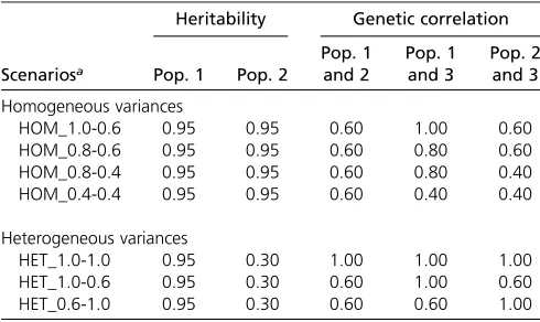
Scenarios:Seven different scenarios of multipopulation
ge-nomic prediction were investigated, differing in heritabilities and genetic correlations between the populations (Table 1). Thefirst four scenarios represent multienvironment genomic prediction, where populations in different environments were combined in one training population in which SNP ef-fects were estimated. In these scenarios, the variances were assumed to be homogeneous;i.e., heritability was assumed to be the same in each population (0.95), but genetic correla-tions between populacorrela-tions varied from 0.4 to 1. The last three
scenarios represent multitrait genomic prediction, where populations measured for different traits are combined in one training population. In these scenarios, variances were assumed to be heterogeneous; i.e., each population had a different heritability of 0.3 or 0.95, and genetic correlations between populations were 0.6 or 1. The values for the heri-tabilities of 0.3 and 0.95 were chosen to have a clear contrast between the populations.
In each scenario, population 1, population 2, or popula-tions 1 and 2 were used as the training population and population 3 contained the predicted individuals. Each sce-nario was analyzed using both approaches of selecting QTL: RANDOM and LOW MAF. Simulations were replicated 100 times in each scenario.
Calculating Me:Values forMeacross the different
popula-tions were calculated based on the difference between the genomic and the pedigree relationship matrix. Since the subset of SNPs slightly differed between the two ap-proaches of selecting candidate QTL, RANDOM and LOW MAF, values for Me were calculated for each of the
ap-proaches. To reduce the impact of incompleteness of the pedigree, only individuals with at least three generations of complete pedigree were taken into account, resulting in 329 individuals in population 1, 270 individuals in popu-lation 2, and 90 individuals in popupopu-lation 3. Thereafter, an exponential function was fitted through the data to further reduce the impact of an insufficient pedigree depth, as explained before. TheGmatrix was the same for all repli-cates, since the subset of 372,405 SNPs was constant for all replicates while QTL were resampled every replicate, resulting in the sameMefor all replicates. Therefore, only
one accuracy could be predicted for all replicates of the same approach of selecting candidate QTL, repre-senting the expected average accuracy of estimating SNP effects.
Table 1 Overview of the different scenarios to simulate phenotypes
Heritability Genetic correlation
Scenariosa Pop. 1 Pop. 2
Pop. 1 and 2
Pop. 1 and 3
Pop. 2 and 3 Homogeneous variances
HOM_1.0-0.6 0.95 0.95 0.60 1.00 0.60
HOM_0.8-0.6 0.95 0.95 0.60 0.80 0.60
HOM_0.8-0.4 0.95 0.95 0.60 0.80 0.40
HOM_0.4-0.4 0.95 0.95 0.60 0.40 0.40
Heterogeneous variances
HET_1.0-1.0 0.95 0.30 1.00 1.00 1.00
HET_1.0-0.6 0.95 0.30 0.60 1.00 0.60
HET_0.6-1.0 0.95 0.30 0.60 0.60 1.00
Pop., population.
aScenarios are labeled as follows: The names of the scenarios assuming
Empirical accuracy of genomic prediction: The empirical accuracies of genomic prediction were obtained both with a single-trait and with a multitrait Genomic Best Linear Un-biased Prediction (GBLUP) type of model run in ASReml (Gilmouret al. 2009), using the simulated phenotypes and including population as a fixed effect. Genomic values for the predicted individuals were estimated using a genomic relationship matrix,G, containing all training and predicted individuals and simulated phenotypes of the training individ-uals. The G matrix included in the models was calculated using the allele frequencies across all individuals without taking the population into account. The other steps in calcu-latingGwere the same as explained above.
In the single-trait model, variances were estimated using Residual Maximum Likelihood (REML). Therefore, the model used was termed Genomic-Relatedness-Matrix Residual Max-imum Likelihood (GREML) instead of GBLUP, where vari-ances are assumed to be known. In the single-trait model, the phenotypes of the different populations were pooled in one population, without taking the genetic correlations between the populations into account. The differences in heritability were, however, taken into account by weighting the pheno-types differently and in this way acknowledging that the phenotypes in one population were more accurately repre-senting the genomic values of the individuals compared to the phenotypes in the other population. It was assumed that the heritability of the phenotypes from the population with the lowest heritability,i.e., a heritability of 0.3, represented the trait heritability based on one measurement. The phenotypes of individuals from this population were given a weight of 1. The heritability of the other population,i.e., a heritability of 0.95, represented the heritability based on multiple measure-ments of the same trait. In other words, it represented the reliability of the phenotype based on more than one record. This indicates that the genetic variance can be assumed to be the same in both populations. The weight for the phenotypes of individuals from the population with the highest reliability (r2) was equal to the ratio of the residual variances in both
populations, which can be calculated as
w¼ 12h
2
h2=r22h2: (22)
Following Equation 22, a weight of 44.33 was given to the phenotypes from the population with a heritability of 0.95. One possible scenario where phenotypes could be weighted differently is in dairy cattle populations, where phenotypes of cows are generally based on one single measurement and phenotypes of bulls are based on different numbers of progeny, for which the same weights can be obtained following Garrick et al.(2009).
The multitrait model considered the phenotypes for the same trait in the different populations as different traits with a genetic correlation between the traits. Estimating all genetic correlations in the multitrait model was not possible, since phenotypes of the predicted individuals were not included in
the model. Therefore, genetic correlations and variance com-ponents were assumed to be known andfixed to the simulated values, and the multitrait model was termed GBLUP.
For each of the models, the accuracy of genomic prediction was calculated as the correlation between the simulated TGVs and predicted genomic values. Note that the single-trait and multitrait GBLUP models use both SNP information and simulated phenotypes that differed across the replicates. Therefore, averages and standard errors across the replicates were calculated and compared to the predicted accuracies.
Evaluating the potential accuracies of two scenarios
The derived equation can be used to investigate the accuracy of different scenarios of multipopulation genomic prediction. To show this, we used Equation 18 to evaluate the potential accuracy for two specific scenarios, assuming that all genetic variance in the predicted population was captured by the SNPs in the training population (rLDA;C =rLDB;C = 1). Thefirst
sce-nario is relevant for dairy cattle breeding, where bulls with deregressed estimated genetic values based on daughter in-formation are in general used in the training population, with a heritability equal to the reliability of the estimated genetic values. Different studies have investigated the potential to increase the accuracy of genomic prediction by adding cows to the training population with their own phenotypes, which are in general less reliable than estimated genetic values (e.g., Caluset al.2013; Cooperet al.2015). In Equa-tion 18 different numbers of cows (range 0–50,000) were added to a training population of 10,000 bulls, assuming a heritability of 0.05 for the phenotypes of cows that repre-sents the heritability of a fertility trait in dairy cattle (e.g., Karouiet al.2012), different reliabilities (range 0–1) for the estimated genetic values of bulls, and a genetic correlation of 1 between the estimated genetic values of bulls and the phenotypes of cows. The values forMewere set to the values
derived from the cattle genotype data used in this study. The second scenario is based on human studies, in which it was assumed that different numbers of individuals from a population of African descent (range 0–100,000) were added to a training population of 5000 individuals of European de-scent to increase the accuracy of predicting genetic risk for the European population. As an example, parameters for the trait schizophrenia were used, with a heritability of 0.28 in the European population, a heritability of 0.24 in the African population, and a genetic correlation of 0.66 between the populations (De Candiaet al.2013). TheMein the European
population (MeA;Cin Equation 18) was set to 43,000, based on
the equationMe¼2NeL=lnð4NeLÞ(Goddard 2009), an
effec-tive population size (Ne) of 10,000 (McEvoyet al.2011), and
a genome length (L) of 30 M (Venteret al.2001). TheMe
across the populations (MeB;C in Equation 18) was varied
(range 43,000–2,000,000).
Data availablity
doi.org/10.5061/dryad.1525t. File Genotypes_422405SNPs contains the genotype for each individual. File Pedigree con-tains the pedigree for each individual. File ID_Population contains the division of the individuals over the populations. File Phenotypes_QTL_RANDOM contains the simulated phe-notypes for each individual for the RANDOM scenario. File Phenotypes_QTL_LowMAF contains the simulated pheno-types for each individual for the LOW MAF scenario.
Results
In this section, the results of the prediction equation arefirst presented assuming that all genetic variance in the predicted population (population 3) is captured by the SNPs in the training population. These predicted accuracies were used to calculate rLD1;3 andrLD2;3 based on the ratio between the empirical and the predicted accuracy of genomic prediction when only one of the populations, population 1 or population 2, was used as the training population. As a next step, the calculated values forrLD1;3andrLD2;3were used to predict the accuracy of genomic prediction when populations 1 and 2 were combined in the training population.
Calculating Me
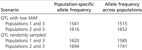
In Table 2, the different estimatedMevalues across
popula-tions are shown. Due to only small differences in the subset of SNPs used to calculate G, estimated Me values were very
similar for the scenarios with QTL randomly sampled (RAN-DOM) and QTL sampled with a low MAF (LOW MAF). Using population-specific allele frequencies or allele frequencies across populations had only a very small effect on the esti-mated values forMe, as well as on the predicted accuracies
(range20.9%–1.3%). This indicates that, for this study, the use of population-specific allele frequencies or the allele fre-quency across populations did not influence the results, due to the very similar allele frequencies across the three popu-lations. Therefore, the predicted accuracies are shown only for theMevalues calculated based on aGmatrix using the
allele frequencies across the populations.
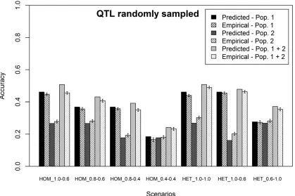
Scenarios with QTL randomly sampled (RANDOM)
In this section, results are presented for the RANDOM sce-narios of simulating phenotypes. For these scesce-narios, the predicted accuracies and average empirical accuracies of
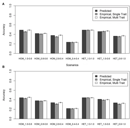
genomic prediction obtained with a single-trait model using either a single or a combined training population and different scenarios of simulated phenotypes are shown in Figure 2. The
first four scenarios show the accuracies when different genet-ic correlations between the populations were simulated, with the same heritability in each of the populations. These sce-narios show that when only one population was used as a training population, predicted and empirical accuracies were, as expected, higher when the genetic correlation between training and predicted individuals was higher. There was only a small difference between the accuracies obtained us-ing population 1 or 2 as the trainus-ing population when the genetic correlation with the predicted individuals was the same, because both populations were about equally related to the predicted individuals. Combining the two populations in one training population always resulted in an increase in both predicted and empirical accuracies. The magnitude of the increase in accuracy depended on the genetic correlation between the predicted individuals and the added population; the higher the genetic correlation, the higher the increase in accuracy.
The last three scenarios show the predicted and empirical accuracies, using different heritabilities in each of the ulations and genetic correlations of 1 and 0.6 between pop-ulations. These scenarios show that when only one population was used as the training population, predicted and empirical accuracies were, as expected, higher when the heritability in the training population was higher. For this study, a herita-bility of 0.3 resulted in60% of the accuracy obtained with a heritability of 0.95. Adding 450 individuals from the popula-tion with a low heritability to a training populapopula-tion of 450 individuals from the population with a high heritability, how-ever, still resulted in an increase in accuracy. The increase in both predicted and empirical accuracies was again lower when the genetic correlation was lower, similar to the scenar-ios with the same heritability in each population.
For each of the scenarios, the predicted accuracy of geno-mic prediction shown in Figure 2 is assuming thatrLD1;3 = rLD2;3= 1. In general, predicted accuracies were very slightly overestimating the empirical accuracies of genomic predic-tion (61%), both when the heritability was the same in each population and when the heritability was different. When population 1 was used as the training population, the over-estimation was on average 4% (range 1–11%). When popu-lation 2 was used as the training popupopu-lation, the empirical accuracy was slightly underestimated by the predicted accu-racy by on average 8% (range220% to22%). When both populations were combined in the training population, the overestimation was on average 6% (range 3–12%). These results indicate that when QTL were randomly sampled from the SNPs, most of the genetic variance in the predicted indi-viduals was tagged by the SNPs in the training population, especially when population 2 was used as the training population, and the estimated value for rLD1;3 = 0.96 and for rLD2;3 = 1. Using these calculated values to predict the accuracy of genomic prediction for the combined training Table 2 EstimatedMevalues across populations, using
population-specific allele frequencies or the allele frequency across populations to set up G
Scenario
Population-specific allele frequency
Allele frequency across populations
QTL with low MAF
Populations 1 and 3 1541 1515
Populations 2 and 3 1616 1652
QTL randomly sampled
Populations 1 and 3 1620 1585
population reduced the overestimation of the empirical accu-racy to 3%.
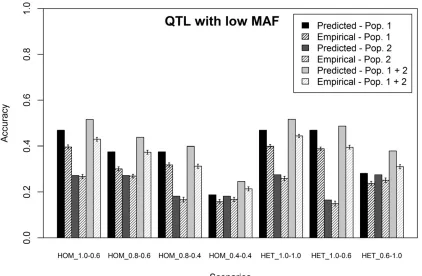
Scenarios sampling QTL with low MAF (LOW MAF)
In this section, results are presented for the LOW MAF sce-narios of simulating phenotypes. For these scesce-narios, the predicted and average empirical accuracies of genomic pre-diction obtained with a single-trait model using either a single or a combined training population are shown in Figure 3, assumingrLD1;3=rLD2;3 = 1. All empirical accuracies for the LOW MAF scenarios were lower than the accuracies obtained for the RANDOM scenarios. The predicted accuracies, how-ever, were similar to the predicted accuracies for the RANDOM scenarios. So, the predicted accuracies for the LOW MAF sce-narios overestimated the empirical accuracies to a greater ex-tent. On average, the overestimation was 615% and again higher when population 1 was used as the training population, compared to using population 2 as the training population (population 1, 20%; population 2, 7%; combined training pop-ulation, 20%). These results indicate that, as expected, a smaller proportion of the genetic variance in the predicted individuals was tagged by the SNPs in the training population when QTL were sampled with a low MAF and the estimated value forrLD1;3 = 0.84 and forrLD2;3 = 0.94. Using these cal-culated values to predict the accuracy of genomic prediction
for the combined training population reduced the overestima-tion of the empirical accuracy to 5%.
Single-trait vs. multitrait model
rLD1;3 and rLD2;3 reduced on average across replicates to 0% (range22% to +2%) for the RANDOM scenarios and to 1% (range22% to +3%) for the LOW MAF scenarios. This indi-cates that the equation can accurately predict the accuracy of genomic prediction when the proportion of the genetic vari-ance in the predicted population not captured by the SNPs in the training population is known and taken into account.
The potential accuracies of two scenarios
The potential accuracies when cows with their own pheno-types were added to a training population of 10,000 bulls with deregressed estimated genetic values are shown in Figure 5, for different numbers of cows added to the training popula-tion and different reliabilities for the estimated genetic val-ues. Figure 5 shows that when the reliability of the estimated genetic values of the bulls was low, a relatively small amount of cows had to be added to the training population to see a substantial increase in accuracy. When the reliability of the estimated genetic values was high (.0.7), a high accuracy was already obtained with 10,000 bulls in the training pop-ulation (accuracies were .0.9), and enlarging the training population by adding cows with their own phenotypes resulted in only a minor increase in accuracy.
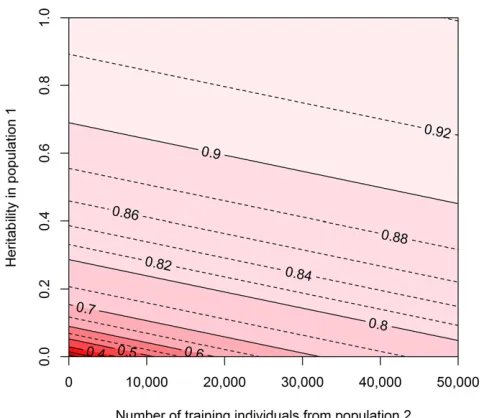
The potential accuracies for the human scenario where a population of African descent was added to a training
population of European descent to predict the genetic risk of individuals from the European population are shown in Figure 6, with different numbers of individuals from the African population added to the training population and different values for Me across the populations. Figure 6 shows that
whenMeacross the two populations was low, adding
individ-uals from another population could substantially improve the accuracy of predicting genetic risk. When the Me across
the two populations was large (.20 times the Me within
the European population), adding individuals from the other population resulted in only a minor increase in accuracy. This indicates that to improve the accuracy of predicting genomic values, using training individuals from populations that are more closely related and have a more consistent LD pattern, resulting in lower values forMeacross populations, is more
beneficial than using training individuals from populations that are only distantly related.
Discussion
prediction when the proportion of the genetic variance in the predicted population captured by the SNPs in the training population was known and taken into account. In addition to being able to deal with differences in heritability in each population and genetic correlations between populations different from 1, the equation can in principle handle data from more divergent populations, such as populations from different environments, breeds, or lines. The proportion of the genetic variance captured by the SNPs can, however, be expected to be lower across more divergent populations, as is discussed later. To confirm that the equation indeed gives accurate predictions for those other scenarios when the pro-portion of the genetic variance captured by the SNPs is
known, further validation of the equation is required, using a broader range of populations, preferably with real genotype and phenotype information.
Potential of the derived equation
The equation gives insight into important parameters for multipopulation genomic prediction and can be used to com-pare different scenarios. The equation, for example, shows that when theMeacross populations is two times higher than
Mewithin a population, two times more individuals from the
variance can be captured. When these last criteria are not met, even more individuals from the other population have to be added to obtain the same increase in accuracy.
The equation can also be used to investigate the potential accuracy of different scenarios, as was done in Figure 5 and Figure 6. In Figure 6, the equation was applied to a scenario where human populations of European and African descent were combined in one training population to predict schizo-phrenia risk for the European population, a scenario that was suggested by De Candiaet al.(2013). The results show that when the LD pattern is very different across populations, resulting in a highMeacross populations, it is very unlikely
to see an increase in prediction accuracy, even when a lot of individuals from the other population are added. Moreover, they show that the sensitivity of the accuracy forMeis much
smaller at larger values ofMeacross populations compared to
small values ofMe, which is in agreement with the results
found within a population (Brard and Ricard 2015). Evalua-tion of such scenarios requires that estimates for the input parameters, such as the Me across predicted and training
populations, the heritability of the trait in each of the training populations, the genetic correlations between the popula-tions (rG), and the part of the genetic variance in the
pre-dicted population captured by the SNPs in the training population (rLD), should, however, be known. Apart from
the heritability, for which estimates are straightforward to calculate, each of the input parameters and how to estimate values for those parameters are discussed in more detail in the following paragraphs.
Effective number of chromosome segments (Me)
In the derived prediction equation,Meacross populations is
an important parameter. This parameter can be interpreted as a statistical concept and represents the effective number of segments that are segregating in a combined population, which is a measure for the effective number of effects that has to be estimated in one population to predict genomic values for individuals from another population. It depends on the consistency in LD between the populations; when the LD pattern is completely different between the populations, each of the segments has to be very small to segregate in both populations, resulting in a largeMeacross the populations.
It is of note that the derived equation assumes that Me
segments are underlying the trait and that each segment explains an equal amount of the genetic variance. This indi-cates that the equation is basically assuming an infinitesimal model. The GBLUP model also assumes an infinitesimal model, and therefore theMerepresents the number of effects
that have to be estimated in a GBLUP model and the pre-diction equation is able to accurately predict the accuracy from a GBLUP type of model. In a Bayesian variable selection Figure 5 Predicted accuracies with different numbers of individuals from
population 2 added to a training population consisting of 10,000 individ-uals from population 1 with different heritabilities for the trait. The input parameters represent a scenario in dairy cattle where a cow population with their own phenotypes (population 2) was added to a bull population with estimated genetic values based on daughter information (population 1). Due to different numbers of daughters used to estimate genetic values for the bulls, the heritability or reliability of the phenotype in population 1 ranged between 0 and 1. The heritability for the trait in population 2 was 0.05, and genetic correlations between the training populations and be-tween both training populations and the predicted population were 1. The values forMewere equal to the values in the simulations (Me1;3 = 1620,Me2;3 = 1694).
Figure 6 Predicted accuracies with different numbers of individuals from population 2 added to a training population consisting of 5000 individ-uals from population 1 with different values for the effective number of chromosome segments,Me, across populations 1 and 2. The input pa-rameters represent a human scenario where a population of African de-scent (population 2) was added to a population of European dede-scent (population 1) to predict the genetic risk for schizophrenia in the Euro-pean population (population 3 = population 1), with heritabilities of 0.28 in population 1 and 0.24 in population 2 and a genetic correlation of 0.66 between populations 1 and 2 (De Candiaet al.2013). TheMein pop-ulation 1 was set to 43,000, based on the equationMe¼2NeL=lnð4NeLÞ (Goddard 2009) and an effective population size of 10,000 (McEvoyet al.
model, the number of effects that have to be estimated can be lower thanMefor traits where the effective number of QTL
underlying that trait is lower thanMe(Daetwyleret al.2010;
Van Den Berget al.2015). This indicates that when the num-ber of QTL is substantially lower than Me and a Bayesian
variable selection model is used, the number of estimated effects is equal to the effective number of QTL, which is the value that should be used in the equation to predict the ac-curacy of genomic values.
Within a population, the value forMe can be estimated
based on the effective population size (Goddard 2009; Hayes et al. 2009b; Goddardet al. 2011), as well as using the re-lationship matrices based on genomic information and pedi-gree information (Goddardet al.2011; Wientjeset al.2013). For the Meacross populations, it is not possible to use the
equations based on effective population size and a value for Mecan be estimated based only on the genomic and pedigree
relationship matrices. In the prediction equation, however, the Meacross populations should be known for predicting
the accuracy of genetic values before individuals are geno-typed. For these scenarios, it is possible to estimateMebased
on a small subset of individuals, for example 100 individuals from both populations, for which pedigree and genotype in-formation is available. Another approach would be to esti-mateMebased on the differences between the populations,
since the value for Me across populations depends on the
strength of LD between loci (Goddardet al.2011), which is at least partly different across populations (Sawyer et al. 2005; De Rooset al.2008; Veroneze et al.2013; Wientjes et al. 2015c). The more divergent the populations are, the higher the value forMeacross populations. In this study, the
estimatedMe within a population was1350 for all three
populations and the values forMe across populations were
20% higher. In a study using different closely related cattle breeds, theMevalues across populations were reported to be
10 times larger thanMewithin a population (Wientjeset al.
2015b). This indicates that when very closely related popu-lations are investigated, the Me across populations can be
expected to be 2 times the Me within a population. For
closely related breeds, the Me across populations can be
expected to be 10 times the Me within a population. For
distantly related populations, the value forMeacross
popu-lations can be even higher.
Genetic correlation between populations (rG)
Another input parameter is the genetic correlation between the populations, which is the correlation between the allele substitution effects of the QTL. In a simulation study with at least 100 individuals in each of the populations, it was shown that this parameter can accurately be estimated using a genomic multitrait model, where the same trait in different populations was treated as a different trait (Wientjeset al. 2015b). For closely related populations with an overlapping pedigree, such as populations in different countries that have some common coancestry, the genetic correlation can also be estimated using a pedigree relationship matrix (Schaeffer
1994). For more distantly related populations, such as differ-ent breeds or lines, the pedigree would probably not be deep enough to capture the relationships across populations and a relationship matrix based on genomic information is required (Karouiet al.2012; Huanget al.2014).
Genetic variance captured by the SNPs (rLD)
Results of this study show that the empirical accuracy of genomic prediction depended on the MAF of the QTL un-derlying the simulated trait; when QTL had on average a lower MAF than the SNPs, the accuracy reduced. This is in agree-ment with results of other studies using single-population or multipopulation genomic prediction (Daetwyleret al.2013; Wientjeset al.2015a). The reason for this is a decrease in the strength of LD between QTL and SNPs when the MAF of QTL is lower than the MAF of SNPs (Khatkaret al.2008; Yanet al. 2009; Wientjeset al.2015c), reducing the proportion of the genetic variance captured by the SNPs. As stated before, the MAF of QTL underlying complex traits is expected to be lower than the MAF of SNPs (Goddard and Hayes 2009; Yanget al. 2010; Kemper and Goddard 2012), indicating that it is highly likely that not all the genetic variance can be captured by the SNPs in real data.
The square root of the proportion of the genetic variance captured by the SNPs is represented in the prediction equation asrLDand depends on the density of the SNP chip, the
char-acteristics of the QTL underlying the trait, and the investi-gated populations (Daetwyler 2009; Erbeet al.2013). This parameter can only be estimated based on empirical data, by comparing the predicted and empirical accuracy. Using this approach,rLDwas estimated to be1 when QTL were
ran-domly sampled from the SNPs and0.85 when QTL had a low MAF in this study. In other studies using real data, the square ofrLD,i.e.,r2LD;was estimated to be0.8, using a 50k
chip in Holstein–Friesian dairy populations for net merit (Daetwyler 2009) and production traits (Erbeet al.2013), and was slightly lower in Brown Swiss dairy populations for production traits (Erbeet al.2013; Román-Ponceet al.2014). The studies estimatingr2
LD focused on only one population.
Across populations, the value forrLDis supposed to be lower
and depends on the number of generations since the separa-tion of the populasepara-tions; the higher the number of genera-tions, the lower the consistency in LD (e.g., Andreescuet al. 2007; De Rooset al.2008) and the higher the chance of QTL segregating in only one population (Kemper et al. 2015). Therefore, the values of pffiffiffiffiffiffiffi0:8= 0.89 for rLD found in the
empirical studies can probably be seen as the upper limit of rLD, which can be obtained only when the predicted and
training populations are subsets from the same population. The more divergent the predicted and training populations are, the lower the value ofrLDand the farther away the value
is from the upper limit ofrLDwithin a population.
Single-trait vs. multitrait model
of a multitrait model was beneficial when the genetic correla-tion between the two training populacorrela-tions and the predicted population was different. In an empirical study with three different chicken lines with different genetic correlations be-tween populations, a multitrait model resulted in more or less similar accuracies compared to a single-trait model (Huang et al. 2014). In an empirical study with three dairy cattle breeds, a multitrait model using estimated genetic correlations resulted in more or less similar accuracies compared to a multi-trait model with genetic correlationsfixed at 0.95 (Karouiet al. 2012). Combining dairy cattle populations from three differ-ent countries, however, showed a higher accuracy for a multi-trait model compared to a single-multi-trait model (De Haaset al. 2012). So, empirical studies have shown that multitrait mod-els yield accuracies that are similar to or slightly higher than those of single-trait models; however, genetic correlations were generally estimated with large standard errors.
The observed increase in accuracy of using a multitrait model when genetic correlations between the two training populations and the predicted population were different can be explained as follows. When the genetic correlations are different, it is beneficial to take into account that estimated SNP effects from one training population are more related to SNP effects in the predicted population than estimated SNP effects from the other training population. When the genetic correlation was the same, the use of a multitrait model was not beneficial, even when the genetic correlation among the training populations was different from 1. This can be explained by the fact that estimated SNP effects in each of the training populations are equally related to SNP effects in the predicted population. In the single-trait model, aver-ages of the SNP effects in both training populations are estimated, which have the same correlation with the SNP effects in the predicted population as the SNP effects in each of the training populations. Therefore, taking the genetic corre-lation between the training popucorre-lations into account had no effect on the obtained accuracy for those scenarios.
Conclusion
A deterministic equation is derived to predict the accuracy of genomic values when the training population comprises in-dividuals of different populations, such as populations from different lines or environments or populations measured for different traits. In this study, the equation was validated for different multienvironment and multitrait scenarios. Re-sults showed that the accuracy of estimating genomic values can be accurately predicted for these scenarios, provided that the effective number of chromosome segments across pre-dicted and training populations, the heritability of the trait in each of the training populations, the genetic correlations between the populations, and the proportion of the genetic variance in the predicted population captured by the SNPs in the training population are known. Therefore, the derived equation can be used to investigate the potential accuracy of different multipopulation genomic prediction scenarios and to decide on the most optimal design of training populations.
Acknowledgments
The authors are thankful for useful comments from Chris Schrooten and Henk Bovenhuis. The RobustMilk project and the National Institute of Food and Agriculture are acknowl-edged for providing the 50k genotypes of the Holstein– Friesian cows, and the global Dry Matter Initiative (gDMI) is acknowledged for imputing those to 777k genotypes. This study was financially supported by Breed4Food (KB-12-006.03-005-ASG-LR), a public–private partnership in the domain of animal breeding and genomics, and CRV BV (Arn-hem, The Netherlands).
Literature Cited
Andreescu, C., S. Avendano, S. R. Brown, A. Hassen, S. J. Lamont
et al., 2007 Linkage disequilibrium in related breeding lines of chickens. Genetics 177: 2161–2169.
Brard, S., and A. Ricard, 2015 Is the use of formulae a reliable way to predict the accuracy of genomic selection? J. Anim. Breed. Genet. 132: 207–217.
Calus, M. P. L., Y. De Haas, and R. F. Veerkamp, 2013 Combining cow and bull reference populations to increase accuracy of ge-nomic prediction and genome-wide association studies. J. Dairy Sci. 96: 6703–6715.
Calus, M. P. L., H. Huang, A. Vereijken, J. Visscher, J. Ten Napelet al., 2014 Genomic prediction based on data from three layer lines: a comparison between linear methods. Genet. Sel. Evol. 46: 57. Cooper, T. A., G. R. Wiggans, and P. M. VanRaden, 2015 Short
communication: analysis of genomic predictor population for Holstein dairy cattle in the United States—effects of sex and age. J. Dairy Sci. 98: 2785–2788.
Daetwyler, H. D., 2009 Genome-wide evaluation of populations. Ph.D. Thesis, Animal Breeding and Genomics Centre, Wagenin-gen University, WaWagenin-geninWagenin-gen, The Netherlands.
Daetwyler, H. D., B. Villanueva, and J. A. Woolliams, 2008 Accuracy of predicting the genetic risk of disease using a genome-wide approach. PLoS One 3: e3395.
Daetwyler, H. D., R. Pong-Wong, B. Villanueva, and J. A. Wool-liams, 2010 The impact of genetic architecture on genome-wide evaluation methods. Genetics 185: 1021–1031.
Daetwyler, H. D., M. P. L. Calus, R. Pong-Wong, G. De los Campos, and J. M. Hickey, 2013 Genomic prediction in animals and plants: simulation of data, validation, reporting, and bench-marking. Genetics 193: 347–365.
De Candia, T. R., S. H. Lee, J. Yang, B. L. Browning, P. V. Gejman
et al., 2013 Additive genetic variation in schizophrenia risk is shared by populations of African and European descent. Am. J. Hum. Genet. 93: 463–470.
De Haas, Y., M. P. L. Calus, R. F. Veerkamp, E. Wall, M. P. Coffey
et al., 2012 Improved accuracy of genomic prediction for dry matter intake of dairy cattle from combined European and Aus-tralian data sets. J. Dairy Sci. 95: 6103–6112.
De Los Campos, G., D. Gianola, and D. B. Allison, 2010 Predicting genetic predisposition in humans: the promise of whole-genome markers. Nat. Rev. Genet. 11: 880–886.
De Los Campos, G., Y. C. Klimentidis, A. I. Vazquez, and D. B. Allison, 2012 Prediction of expected years of life using whole-genome markers. PLoS One 7: e40964.