Abstract
HAMILTON, PATRICK. Functional Verification of an ALU Core applying the Constrained Random approach (Under the direction of Dr. Paul D. Franzon)
Biography
Acknowledgements
There is never a job in this world that can be single-handedly done. This work is no exception. Let me begin by naming my advisor, Dr. Paul Franzon, who was always available for any doubt or question, howsoever elementary or trivial they might be. I would like to express my sincere thanks for his guidance, support, patience and his constant encouragement.
I would like to specially thank Mr. John Goss, IBM verification lead, for introducing me to the world of verification. Without his insight and guidance, needless to say, this project would have never got completed. Thank you for your quick responses to my emails.
Also many thanks to, my committee members, Dr. Eric Rotenberg and Dr.Rhett Davis, for their valuable input, encouragement and for reviewing my thesis.
Special thanks to Gaurav Mehta, who worked with me in this project and dedicated many late nights. His contribution played a major role in implementing this project.
I would also like to express my appreciation for my friends, especially my room-mates for always supporting and being there for me at the time of my need.
My sincerest thanks to my parents and family, who even though far away, have never lost hope in me. Special thanks to my father Joseph Pushparaj and mother Hemakalani Caroline who dedicated their entire life working and educating their 2 children.
TABLE OF CONTENTS
LIST OF FIGURES ... vi
LIST OF TABLES ... vii
Chapter 1 Introduction... 1
1.1 Motivation and Contribution... 1
1.2 Thesis Organization ... 2
Chapter 2 The Art of Verification, an Overview ... 3
2.1 Verification vs. Test... 3
2.2 Logic Verification Flow... 4
2.2.1 Conformance Verification Plan ... 5
2.2.1.1 Specifying the Verification... 5
2.2.1.2 Feature Extraction... 6
2.2.1.3 Levels of Verification ... 7
2.2.1.4 Functional Verification Approaches ... 7
2.2.1.5 Verification Strategies ... 9
2.2.1.6 From specifications to testbenches ... 9
2.2.2 The Testbench Environment ... 10
2.2.2.1 Verifying Testbenches ... 11
2.2.3 Coverage and Regression... 12
2.2.3.1 Code and Functional coverage... 12
2.2.3.2 Regression suites and management ... 14
2.2.4 Escape analysis ... 15
Chapter 3 Design under Verification: The ALU core specification ... 16
3.1 Architectural Overview... 16
3.2 I/O Protocols ... 17
3.3 Basic I/O Timing... 18
3.4 Command and ordering rules... 19
3.5 Design Specifications... 19
3.5.1 Cmd_inX... 20
3.5.2 Dispatch/Priority Component ... 21
3.5.2.1 Hold Table details ... 22
3.5.2.2 Global Table details ... 22
3.5.2.3 Good-to-Go Algorithm ... 23
3.5.2.4 Dispatch details... 24
3.5.3 Internal Registers ... 24
3.5.4 ALU Input Stage... 25
3.5.5 Array Write and Output Stage ... 25
Chapter 4 Verification of the ALU core - CVP... 28
4.1 Overview... 28
4.2 Verification Strategy... 28
4.3 Functional Requirements ... 28
4.4 Verification Environment ... 29
4.4.1 Top Level ... 31
4.4.2 Stimulus/Driver... 32
4.4.3 Scoreboard ... 35
4.4.4 Checker ... 37
4.4.5 Coverage information ... 43
4.4.5.1 Coverage points ... 44
Chapter 5 Results: Bugs and Coverage ... 53
5.1 Bugs ... 53
5.2 Coverage Results ... 53
5.2.1 Value Coverage... 53
5.2.2 Cross Coverage ... 54
5.2.3 Additional Crosses... 56
5.2.4 Transitions... 59
5.2.5 Queue Coverage... 60
Chapter 6 Conclusion and Suggestions for Future Work... 61
LIST OF FIGURES
Figure 1.1 Functional Verification paths ... 1
Figure 2.1 Validation of Systems... 3
Figure 2.2 Testing vs. Verification ... 4
Figure 2.3 Verification Cycle ... 5
Figure 2.4 Black–Box Approach ... 8
Figure 2.5 A typical Verification Testbench... 11
Figure 2.6 Redundancy in an ambiguous situation enables accurate verification [1] ... 12
Figure 3.1 Input/Output Interfaces... 16
Figure 3.2 I/O Timing ... 18
Figure 3.3 High level design diagram... 20
Figure 3.4 High level Diagram of Dispatch/Priority ... 21
Figure 3.5 Internal Register I/O... 24
Figure 3.6 Dataflow for Fetch and Branch Commands ... 26
Figure 4.1 Verification Environment... 30
Figure 4.2 Top level Model ... 31
Figure 4.3 Illustration of the calc_exp_res() function ... 36
Figure 4.4 Path taken by VALID instructions ... 37
Figure 4.5 Path taken by INVALID instructions ... 38
Figure 4.6 Information content at each stage... 38
Figure 5.1 Value Coverage of Commands... 53
Figure 5.2 Value Coverage of Tags ... 54
Figure 5.3 Value Coverage of D1 register ... 54
Figure 5.4 Cross Coverage between Commands and Tags... 55
Figure 5.5 Cross Coverage between Tags and R1 (only tag 0 and 1 shown here) ... 55
Figure 5.6 Cross Coverage between Data limit = FFFFFFFF and STORE Command .... 56
Figure 5.7 Cross Coverage between Port ID and Commands ... 56
Figure 5.8 Cross coverage between Commands and Output Responses ... 57
Figure 5.9 Cross Coverage between Tags and Output Responses... 57
Figure 5.10 Cross Coverage of Tags and Port Clashes... 58
Figure 5.11 Cross Coverage of Port IDs and Port Clashes ... 58
Figure 5.12 Transition Coverage of Commands... 59
Figure 5.13 Transition of Tags... 59
LIST OF TABLES
Table 3.1 Hold table... 22
Table 3.2 Global Table ... 23
Table 3.3 Branch Tag Table... 26
Table 4.1 Environment Hold table... 41
Table 4.2 Useful Registers for each command ... 41
Table 4.3 Environment Global table... 42
Table 4.4 Cross Coverage ... 45
Table 4.5 Additional Cross Coverage... 47
Chapter 1
Introduction
1.1 Motivation and Contribution
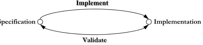
Verification is a process used to demonstrate the functional correctness of a design. [1] The main purpose of “functional” verification is to ensure that a design implements intended functionality. As shown by the reconvergent path model in Figure 1-1, functional verification reconciles a design with its specification.
Figure 1.1 Functional Verification paths
Today’s IC and System-on-Chip (SoC) design trends have placed an immense burden on the shoulders of verification engineers. Processor complexity, custom logic size, software content, and system performance are all increasing at the same time that schedules are being squeezed and resources are stretched. As a result verification consumes about 70% of the design effort [7]. Given the amount of effort, shortage of qualified verification engineers, and the quantity of code that must be produced, it is no surprise that verification rests squarely on the critical path and is the target of new tools and methodologies.
The problem of verification being the bottleneck is the sole motivator for applying the latest concept of constrained random approach in functionally verifying a 32-bit ALU core. An ideal verification flow similar to the design flow has been devised and followed in verifying the core. A whole environment to run the Design Under Verification has been coded and stimuli are driven into the DUV to verify its
Specification RTL
R
RRTTTLLL CCCooodddiiinnnggg
F
functionality. Design has been functionally covered well and bugs determined have been reported to the designer.
The test bench environment was developed using Verisity’s Specman ‘e’ language and the simulations were done using the Specman simulator and Model Technology’s Modelsim.
In this thesis the Courier New font refers to snippets of code used in building and running the testbench environment.
1.2 Thesis Organization
Chapter 2 starts off with a highlight on the art of verification demarcating it from test and covering all the four phases of the logic verification flow from writing the Conformance Verification plan to Escape analysis.
Chapter 3 describes the architecture of the Arithmetic Logic Unit (ALU) core that needs to be verified in detail as per the designer’s specification.
Chapter 4 is where majority of contribution to this thesis lies. It delves into describing the Verification Environment setup to functionally verify the design in detail.
Chapter 5 provides the Results obtained upon verifying the design. Bugs found, their descriptions and coverage analysis results are included in this chapter.
Chapter 2
The Art of Verification, an Overview
2.1 Verification vs. Test
To prevent the faulty behavior of a system designed causing severe damage, it has to be checked whether the system behaves as expected. This process is called validation. To validate a system the desired behavior of the system must be known. A prescription of the desired behavior is called a specification: it describes what a system must do, not how this is done. A system that is supposed to implement the desired behavior is called an
implementation, e.g., a real, executing, piece of hardware [2]. Validation now amounts to checking whether an implementation complies with its specification (see Figure 2.1 [1]).
Two complementary validation techniques that can be used to increase the level of confidence in the correct functioning of systems as prescribed by their specifications are
testing and verification.
Figure 2.1 Validation of Systems
Testing is very often confused with verification. The purpose of the former is to verify that the design was manufactured correctly and to determine any parametric faults or random defects. The purpose of the latter is to ensure that the design meets its functional intent. Figure 2.2 shows the reconvergent paths for both verification and testing [1]. During testing the silicon is reconciled with the netlist that was submitted for manufacturing.
Specification Implementation
I
IImmmpppllleeemmmeeennnttt
V
Figure 2.2 Testing vs. Verification
There is an apparent paradox between the attention that verification and testing get in usage and research. Whereas most of the research in the area of system validation is concentrated on verification, testing is the predominant technique in practice. People from the realm of verification very often consider testing as inferior, because it can only detect some errors, but it cannot prove correctness; on the other hand, people from the realm of testing consider verification as impracticable and not applicable to realistically-sized systems. [2]
2.2 Logic Verification Flow
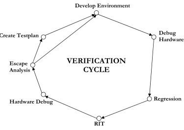
Logic verification or simulation is a process used to demonstrate the functional correctness of a design. It is not an exact science but rather a skill based on the experience gained.
The logic verification flow consists of four reasonable phases:
1. Conformance Verification Plan (CVP) 2. Testbench implementation.
3. Regression and Coverage. 4. Escape Analysis.
The following figure shows a typical Verification Cycle.
H
HHWWWDDDeeesssiiigggnnn
Netlist
M
MMaaannnuuufffaaaccctttuuurrriiinnnggg
Silicon
T
TTeeessstttiiinnnggg V
VVeeerrriiifffiiicccaaatttiiiooonnn
Figure 2.3 Verification Cycle
2.2.1 Conformance Verification Plan
2.2.1.1 Specifying the Verification
Verification requires a lot of planning to be successful, it is important to know where to allocate the resources and what the critical parts of the design are. For this purpose the ASIC design specification is used to produce a list of features and modes that need to be tested. This list of features is then turned into a conformance verification plan (CVP)[5] by specifying testcases that exercise and test that specific feature or function [3]. These testcases focus on specific functionality, which is why they are sometimes referred to as directed tests. A device is said to conform with the specification if it passes all the tests. These tests verify top-level features, since the device is treated as a black-box. A testcase is a part of the testbench, it is an application usually written in the same language as the behavioral model. It runs as one or several processes using the generators and monitors of the testbench to stimulate the design and check for the expected behavior. The result of the simulation run of the test case is passed or failed, but a lot more information is stored for debugging purposes [1]. It is important for the testcase to be able to produce a
RIT
Regression Debug Hardware Develop Environment
Hardware Debug Escape
Analysis Create Testplan
simple result that makes it possible to run regression test suites where all testcases are run, the result then can easily be identified.
Overall the verification plan is a specification document for the verification effort [1]. It provides a forum for the entire design team to define what first-time success is. From the verification plan, a detailed schedule can be created. The entire design team has a stake in the verification plan and they must contribute to it, to make sure that it is complete and correct.
2.2.1.2 Feature Extraction
Features to be verified are extracted from both the text of the design specification and supporting standards documentation, and from any example waveforms in the design specification and/or supporting standards documentation. Since textual descriptions are often more likely to be misinterpreted than waveforms, the waveforms provided a convenient second level of features. The extracted features are listed in the actual verification plan, to be kept as a separate document since it will be a ‘living document’.
2.2.1.3 Levels of Verification
Verification can be performed at various granularities:
• Unit/sub-sub unit level
• ASIC/FPGA/Reusable component level
• System/sub-system/SoC level
• Board level
There are several tradeoffs to decide what levels to perform verification. The smaller ones offer more control and observability but there is more effort to create more environments. Larger ones, the integration of the smaller partitions are implicitly verified at the cost of lower control and observability but less effort because of fewer environments. What ever level is decided, those pieces must be stable and possess a specification document.
In an ideal world, every macro would have ‘perfect verification’ performed meaning all permutations would be verified based on legal inputs and all outputs checked on the small chunks of the design. Unit, Chip and system level would then only need to check interconnections. But in practice, Macro verification across and entire system is not feasible since the business cannot support the development expense considering the macros on a chip and the number of verification engineers required.
2.2.1.4 Functional Verification Approaches
Functional verification can be approached through three complimentary but different approaches: black-box, white-box, and grey-box.
knowledge of its structure and implementation. Hence this method suffers from obvious lack of visibility and controllability.
Figure 2.4 Black–Box Approach
The advantage of black-box verification is that it does not depend on whether the design in implemented in a single ASIC, multiple FPGAs, a circuit board, or entirely in software. A black-box functional verification approach forms a true conformance verification that can be used to show that a particular design implements the intent of a specification regardless of its implementation.
To verify a black box, a verification engineer needs to understand the function and be able to predict the outputs based on the inputs. The black box can be a full system, a chip, a unit of a chip, or a single macro.
In a white-box approach, as the name suggests, it has full visibility and controllability of the internal structure and implementation of the design being verified. This method has the advantage of being able to quickly set up an interesting combination of states and inputs, or isolate a particular function since it has intimate knowledge and control of the internal signals of a design. However, it is tied to a specific implementation and cannot be used on alternative implementations or future re-designs.
Grey-box verification is a black box testcase written with full knowledge of internal details. Grey-box approach controls and observes a design entirely through its top-level interface. However, the particular verification being accomplished is intended to exercise significant features specific to the implementation.
Some piece of logic design
written in Verilog/VHDL
2.2.1.5 Verification Strategies
Given the functionality the strategy for carrying out verification needs to be decided. Strategy involves deciding the level of granularity, the type of test cases, the approach depending upon the visibility and knowledge of the internal implementation of each unit under verification and the method to verify the response.
Verifying the response is relatively difficult, time-consuming and error-prone compared to applying the stimulus. Determining the expected response and then verifying whether the design provided the expected response requires proper planning. The outputs are generally verified using self-checking testbenches but there are a few responses that are more easily recognized right or wrong by a visualizing. It is very important to detect errors as early as possible [1].
A strategy used for system-level verification is random verification, where the inputs are subjected to valid individual operations. The sequence of these operations and the content of the data transferred are random. These simulations would help to create conditions (unexpected or corner cases) missed out in the verification plan. Random simulations are complex to specify and code and hence are used only at the system level. Smaller partitions can take advantage of a single random simulation environment. Based on the verification plan, source code and functional coverage metrics, the random simulation is tuned and constrained into individual testcases.
2.2.1.6 From specifications to testbenches
After enumeration comes prioritization since not all features are created equal and some features are a must-have for the design to properly function or meet the demands of the market. The less important features receive less attention while still others are verified only as time allows [1].
The features are then grouped into testcases to maximize productivity as they require the same configuration, granularity or verification strategy to perform verification. Some testcases may be created based on the coverage metrics (both functional and code coverage). Each test case should have one or more features to claim. The sequence and characteristics of the stimulus for the testcase must also be described. Every testcase should include some error injection mechanism to make sure that errors are detected and reported by the testbench.
Just like features, testcases fall into groups that require similar configuration of the design, use of same abstraction level for the stimulus and response, generate same stimulus, determine validity of a response using a similar strategy, or verify closely related features. The testcases are then finally grouped into testbenches and each group is allocated to a verification engineer who is responsible for implementing the testbench according to its specification [1].
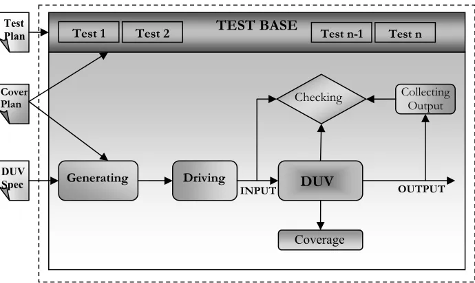
2.2.2 The Testbench Environment
Figure 2.5 A typical Verification Testbench
2.2.2.1 Verifying Testbenches
The purpose of verification effort and writing testbenches is to verify that a design meets its specification. Testbenches include temporary code structure to by-pass large sections to speed up the debugging of a critical section. The testbenches need to be verified that they implement their specification. This can be done by using broken design models or through redundancy. Through the former strategy, each feature needs a broken model. By running these broken models, the test bench could be debugged. Using the broken models to verify test benches is not feasible because of the complexity of managing a large number of controlled and known failure modes inside a design.
The other way, redundancy, i.e., to verify test benches through peer reviews. Having other verification engineers to review that the testbenches implement the specification of the testcases they contain can be a costly alternative but it is far less compared to the cost of a later re-design or replacement of a defective product [1].
TEST BASE
Test 1 Test 2 Test n-1 Test n
DUV
Collecting Output
Checking
Coverage
DUV Spec
Cover Plan
Test Plan
Generating Driving
Figure 2.6 shows the re-convergent path model where redundancy is used to guard against misinterpretation of an ambiguous specification document.
Figure 2.6 Redundancy in an ambiguous situation enables accurate verification [1]
2.2.3 Coverage and Regression
2.2.3.1 Code and Functional coverage
The magnitude and complexity of recent designs introduce new challenges. Two such major challenges are how to reduce the time it takes to do verification to a reasonable size, and how to ensure complete verification.
As exhaustive tests are practically impossible, the verification engineer should spend his time carefully so that unnecessary repetitions are avoided. The engineer needs to be able to answer questions like: Were all possible stimuli variations injected? Were all possible results achieved? Were all Device Under Test (DUT) states visited? Did all the internal transitions take place? Did all the interesting events occur? [4]
The second challenge is to ensure completeness – how can we tell that verification is done? This decision is usually accompanied with tension and the emotional stress of trying to organize the abundant information gathered throughout the recent simulation sessions. Taping out an immature design can have an impact at both the personal and corporate levels.
RTL coding
Verification Interpretation
Interpretation
For these purposes few coverage metrics have been used to evaluate the verification process. Coverage is any metric of completeness with respect to a test selection criterion. The main goals behind coverage are:
• Measure the quality of a set of tests.
• Supplement the test specifications by pointing to uncovered areas.
• Help create regression suites.
• Provide a stopping criterion for verification.
There are mainly two broad categories in coverage:
• Code Coverage
• Functional Coverage.
Code coverage is a technique applied to the DUT to determine how thoroughly the RTL has been exercised using numerous metrics [8].
The basic assumption of code coverage is that unexercised code potentially bears bugs - the code is guilty until proven innocent. One needs to be adventurous to synthesize and tape-out un-exercised logic. That makes code coverage analysis a necessity.
It comprises of:
a. Block coverage: Measures if every sequential block has been executed.
b. Path or Branch coverage: measures if all possible “if/then/else” branch combinations have been exercised.
c. Expression coverage: Measures if all the terms of a Boolean or arithmetic expression have been exercised.
Code coverage checks how well your RTL code was exercised, rather than how well your design functionality was exercised. Therefore, code coverage is a necessity, but not a complete metric. Code coverage should be employed as part of a more comprehensive coverage strategy.
hidden from the report reviewer. Functional coverage elevates the discussion to specific transactions or bursts without overwhelming the verification engineer with bit vectors and signal names. This level of abstraction enables natural translation from coverage results to test plan items [6].
As functional and code coverage are complementary in nature, a tool or methodology which combines both approaches is extremely beneficial.
2.2.3.2 Regression suites and management
A regression suite ensures that modifications to the design remain backward compatible with previously verified functionality. Many times, a change in the design made to fix a problem detected by a testcase, will break functionality that was previously verified. Complete regression test suites are run on a regular basis on the RTL model to verify functionality added and to make sure nothing already tested and debugged has been broken.
Though regression testing can be performed manually, an automated test suite is often used to reduce the time and resources needed to perform the required testing. As individual self-checking testbenches are completed, they are added to a master list of test cases included in the regression simulation. The regression simulation is run at regular intervals. A regression script invokes each testcase in the regression test suite using the simulation configuration script which in turn is used to invoke individual simulations. If the number and duration of testcases in the regression suite make it impossible to run a regression simulation in the allotted time, parallel simulations should be considered. Parallel simulations are maintained using utilities such as pmake, Load Balancer or LSF. Before running a regression, the source control database is to be checked to possess copies of code tagged as being suitable for regression testing. A regression run should not be wasted on files that were not properly debugged.
prevent a testcase from hanging a regression simulation, a timebomb is included in all simulations [1]. This timebomb goes off after a delay long enough to allow the normal operations of the testcase to complete without interruption.
Once a regression simulation is completed, the success or failure of each testcase in the regression suite is checked using an output log scan script. The final single regression report summarizes all the testcase results outlining which particular testcase was successful or failed.
2.2.4 Escape analysis
Chapter 3
Design under Verification: The ALU core specification
3.1 Architectural Overview
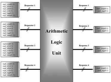
The Arithmetic Logic Unit design is a 32-bit, dual-pipe ALU with 16 internal data registers and four Input/Output ports. Each of the four input ports (called requestors) comprises of the command (reqX_cmd) or the operation to be performed, the register locations of the first and second operands (reqX_d1, reqX_d2), the result register location (reqX_r1), the tag identifier(reqX_tag) and the data to be stored in a specified register (reqX_data) on a STORE command. The output response (outX_resp) and the tag identifier (outX_tag) are the result at each output port with a data output (outX_data) being the result of a FETCH command.
The Input/Output interface schematic is as depicted in Figure 3.1.
Figure 3.1 Input/Output Interfaces
Arithmetic operands are not sent by the requestor as they used to be in an earlier version of this design. The operand data is internally read from the registers. Each requestor can send up to 4 commands with a two-bit tag. Hence (theoretically) the ALU could be working on up to 16 commands at a single time. Since there are two 16 deep internal pipelines in the ALU (one for adds/subs/branches and one for shifts/fetches/stores), it is possible for commands to be executed out of order. For example, if the four ports all send in 3 add commands followed by a shift command, the shift commands are likely to be completed prior to the latter add commands. However, commands from the same port that use the same pipeline (add/sub or shift) will return in order. In order to correspond the responses to the correct commands, a two-bit tag is present at the input and output protocols. Using the same tag simultaneously is not supported i.e. for each requestor the tag per command that is in the pipeline must be unique. The response per pipeline is on a first come first serve basis. Each requestor sends an instruction stream.
3.2 I/O Protocols
For each requestor ‘X’ the following are the input and output protocols:
Inputs:
1. reqX_cmd(0:3)
a. add: 0001 adds contents of d1 to d2 and stores in r1
b. subtract: 0010 subtracts contents of d2 from d1 and stores in r1
c. shift left: 0101 shifts contents of d1 to the left by d2(27:31) places and stores in r1
d. shift right:0110 shifts contents of d1 to the right by d2(27:31) places and stores in r1
e. store: 1001 stores reqX_data(0:31) into r1
f. fetch:1010 fetches contents of d1 and outputs it on out_dataX(0:31) g. branch if zero: 1100 skip next valid command if contents of d1 are 0 h. branch if equal: 1101 skip next valid command if contents of d1 and d2
2. reqX_d1(0:3) 3. reqX_d2(0:3) 4. reqX_r1(0:3) 5. reqX_tag(0:1) 6. reqX_data(0:31)
Outputs:
1. outX_resp(0:1)
a. Successful completion: 01 b. Overflow/Underflow error: 10 c. Command skipped due to branch: 11
2. outX_tag(0:1) 3. outX_data(0:31)
3.3 Basic I/O Timing
The following diagrams in Figure 3.2 represent the valid command input and output and their timing responses.
3.4 Command and ordering rules
Within each requestor’s (port’s) instruction stream, operations can complete out of order with the following restrictions:
1. Operands (d1, d2) cannot be used if prior instruction in stream writes (result r1) to the operand and prior instruction has not completed.
2. Results (r1) cannot be written if either of the prior command’s operands (d1, d2) uses the same register as R1.
3. Same R1 (result) values from different instructions must complete in order.
There are no restrictions of this type across different requestors. For overflow/underflow conditions, the result register, r1, will not be updated.
Following are the rules for commands that follow a branch: 1. Any command can follow a branch
2. If the branch evaluates true, the following command will be "skipped": a. Add/Sub/SL/SR will not write to array
b. Store will not write to array c. Fetch will not return data
d. Branch will evaluate to false (case of branch followed by branch) 3. Response code of '11'b for follower indicating above action has occurred
3.5 Design Specifications
Figure 3.3 High level design diagram
The following are the High level components of the ALU design:
3.5.1 Cmd_inX
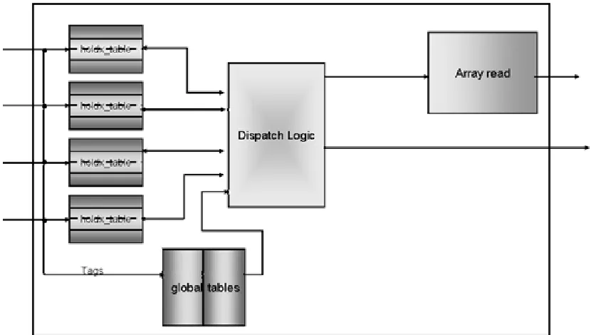
3.5.2 Dispatch/Priority Component
This is the major control block of the design where the priority/dispatch logic resides. It includes the two 16-deep pipelines where commands received from the hold registers are sent to. The following are a few rules regarding the dispatch and priority component:
a. The component cannot dispatch add and shift from the same requester on the same cycle because responses would overwrite each other at the output.
b. It cannot allow a read when there's a write the same cycle to same register. c. A branch's "following" command must be dispatched AFTER the branch.
Figure 3.4 represents a high-level diagram of the Dispatch/Priority component.
3.5.2.1 Hold Table details
Each hold table contains the following fields as shown in Table 3.1
Tag D1(0:3) D2(0:3) R1(0:3) Valid Cmd(0:3) GTG1(0:2) GTG2(0:2) GTG3(0:2)
00
01
10
11
Table 3.1 Hold table
The command’s tag is used to index the table. As a command enters the hold table, the previous commands are searched for register conflicts that will block the new command. Any conflicts are entered into the “Good_To_Go” field (GTG) with a valid bit and the tag bit of the command that will block this new command.
Up to 3 valid bit/tag fields may be set for each command (there can be only 3 cmds in front of the new one. As a command is dispatched, its tag should be cleared from any other command's "good_to_go" fields. When a command is not blocked by other commands (as indicated by no valid entries in good_to_go), then it can be dispatched.
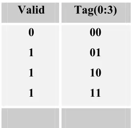
3.5.2.2 Global Table details
There are two global tables which are 16 deep representing the pipelines one for add/sub/branches and the other for shifts/fetches/stores.
Each global table contains the following fields shown in Table 3.2
Valid Tag(0:3)
0 1 1 1
00 01 10 11
Table 3.2 Global Table
The global table is used to identify the oldest commands. The command closest to the top that is “good_to_go” is dispatched. As a command is dispatched, each command below it in the table moves up 1 place.
3.5.2.3 Good-to-Go Algorithm
Within each requestors hold table, good_to_go is set as a command arrives. For each command already in the hold table:
1. If D1|D2|R1 from new command is equal to R1 from command in hold table then set good_to_go with valid bit and previous command’s tag. (program ordering). 2. Turn valid bit off as a previous blocking command is dispatched.
a. D1|D2|R1 not equal to prior R1 in own hold table (program ordering) b. D1|D2 not equal to either of next cycle’s write (no read and write to the
same register on the same cycle)
c. R1 not equal to Shift’s R1 and togglecheck ==0 (two writes to the same register at the same time)
3.5.2.4 Dispatch details
The dispatch will toggle between the global add and global shift in choosing which table has higher priority. The oldest command that is “good_to_go” is selected if it passes these two criteria:
a. D1|D2 not equal to adder or shifter’s next cycle’s writes (no read and write to same register on same cycle).
b. If this global table does not have high priority, then R1 cannot equal R1 of other global table’s dispatched command (protect against simultaneous writes to the same register by both adder and shifter)
When a branch command is received in the hold table, tag is sent to array write units irregardless of when the command is dispatched. The following command is sent as soon as it is received into the hold table.
3.5.3 Internal Registers
The I/O for the internal registers is as shown below in Figure 3.5
Figure 3.5 Internal Register I/O
Internal Registers
Port1_read_valid1 Port1_read_adr1(0:3) Port1_read_valid2 Port1_read_adr2(0:3)
Port1_write_valid Port1_write_adr(0:3) Port1_write_data(0:31) Port2_write_valid
Port1_read_data1(0:31)
Port2_read_valid1 Port2_read_adr1(0:3)
Port2_read_adr2(0:3) Port2_read_valid2
Port2_write_adr(0:3) Port2_write_data(0:31)
Port1_read_data2(0:31)
Port2_read_data1(0:31)
The internal registers have the following access rules: a. No read when writing to same register.
b. Can’t process more than 1 write to the same result register at a time (shifter and adder can’t have same R1 value at the same time).
The Priority/Dispatch logic must protect against violation of these rules. For reads:
a. Data appears on output 1 cycle after read request
b. Up to four reads per cycle (two per port). Can be same address.
c. If there is no read on a port then data 0 is sent. (used for fetches, stores) For writes:
a. Data is valid in array 1 cycle after it is sent.
b. Up to two writes per cycle (one per port). It is up to dispatch to avoid writing to the same address at the same time.
A read and write to the same register on the same cycle will give unpredictable read value.
3.5.4 ALU Input Stage
This stage must latch the tag value and register r1 value for extra cycle and forward to array write component in sync with arith/shift results.
3.5.5 Array Write and Output Stage
The following are the functions of the array write and output stage: a. Gate data to response blocks for fetches.
b. Gate data to registers for adds, shifts and stores
c. Maintain table of outstanding branches and “following” tags
i. Drop “following” commands when branch is true and remove entry ii. Remove entry from outstanding branch table when branch is false iii. Communicate table updates to other array write macro.
Table 3.3 shows all the fields of a Branch Tag table.
Branch tag(0:3) Following tag(0:3) Branch taken Valid
Table 3.3 Branch Tag Table
3.6 Branch Implementation
Figure 3.6 represents the dataflow for branch commands.
Figure 3.6 Dataflow for Fetch and Branch Commands
separately as soon as dispatch receives the commands. The array write macro evaluates the branch result to true or false. Adder’s array write macro will write all entries to the branch table. All the branches are dispatched to the adder and never to the shifter. The array-write units send “1” data to the respective units if the branch evaluates to true. The Array write macro drops the result of the “following” command if the branch was true. In this case no data is written back for stores or arithmetic operations and no data is returned for fetches. A branch following a branch (back-to-back) that has evaluated to true is evaluated to false. The Array write macro does not send response or tag for “following” command to the respective macros.
3.7 Blocking Rules
The following define the out-of-order restrictions:
Case 1: New command operand equals result register of prior command
Command Operand 1 reg Operand 2 reg Result reg
Cmd1 R1 R2 R3
Cmd2 R3 R4 R5
Case 2: New command result register equals operand register of prior command
Command Operand 1 reg Operand 2 reg Result reg
Cmd1 R1 R2 R3
Cmd2 R4 R5 R2
Case 3: New command result register equals result register of prior command
Command Operand 1 reg Operand 2 reg Result reg
Cmd1 R1 R2 R3
Chapter 4
Verification of the ALU core - CVP
4.1 Overview
This chapter deals the verification of the ALU core describing the chosen verification strategy and implementation of this strategy. The design specification was already discussed in detail in Chapter 3. The entire verification effort is described here in the form of a Conformance Verification Plan (CVP).
The ALU design (DUV - device under verification)) takes 4 requestors and will operate on those requests and output their responses onto the respective output bus. This testplan formulates the verification requirements and strategy necessary for 1st pass success. It describes the functions that are to be verified, and what tests will be implemented to verify those functions.
4.2 Verification Strategy
The strategy chosen for this work is a bottom-up grey box verification strategy, using the verification capabilities of Specman ‘e’. Simulations were run using Modelsim. A slightly different flavor of grey-box verification is demonstrated where the ALU block itself is treated as a black-box, but information about the internal communication between blocks and the internal registers was required since they facilitate to locate the root of the error faster.
4.3 Functional Requirements
The following is a list of functions to be verified in the DUV: 1. Supports the add function.
2. Supports the subtract function. 3. Supports the shift left function. 4. Supports the shift right function.
7. Supports the store function. 8. Supports the fetch function. 9. Handles 4 parallel requestors.
10. Outputs successful response for the 8 functions upon valid data. 11. Outputs overflow/underflow response for the add/subtract functions.
12. Outputs a response of 3 if a command is skipped due to a previous branch resolving to true.
13. The command following a branch is skipped if the branch evaluates to true or is not skipped if the branch evaluates to false.
14. When no requests are pending, no response is on the outputs. 15. Outputs correct data for valid fetch operations.
16. Maintains 16 internal data registers.
17. Writes the outputs for the valid commands (add/subtract/store/shr/shl) into the result register at the same cycle that the output response is received.
18. Does not update the data registers if an overflow/underflow condition occurs. 19. Data for fetch operation is valid on same cycle as response
20. Priority logic (for parallel requests) works on first come first serve
21. Priority logic allows 1 add or subtract operation to be dispatched at a time. 22. Priority logic allows 1 shift operation to be dispatched at a time.
23. Priority Logic gives priority to higher number requestor. 24. No requests are lost.
25. Up to 4 requests can be outstanding per requestor.
26. A valid tag corresponding to the tag sent in at the input is received at the output on successful completion of the command.
27. Dispatch logic checks WAR/WAW/RAW conditions correctly.
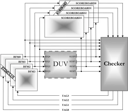
4.4 Verification Environment
used for an encapsulated complex stimulus) is made to operate assuming dynamic partitioning of registers. This helps to reduce the complexity in creating the environment for an otherwise unpartitioned design. The scoreboards combined with a monitor in them snoop data off the input/output lines for calculating expected results and matching them with the actual ones. The scoreboards check whether all the instructions generate correct outputs in terms of data, response and tags. The checker checks the priority structure thoroughly. All constraints on the inputs are imposed in several test cases each. The test cases totally control the data sent to each input port which makes it very easy to modify a test case to test for different bugs.
Figure 4.1 Verification Environment
DUV
Checker
BFM0 BFM1
BFM2 BFM3
SCOREBOARD0 SCOREBOARD1 SCOREBOARD2 SCOREBOARD3
TAG3 TAG2
TAG1
TAG0 REQ0
REQ1 REQ2 REQ3
RESP0
4.4.1 Top Level
The top level comprises of an instance of the ALU environment unit (calc_env under the
sys). It also contains the test case that mainly constrains the number and type of instructions driven by the requestor into the DUV. It also controls the number of requestors and scoreboards to activate (based on number of ports) and randomizes the initial tag sequence thereby additionally checking for errors due to random tag inputs. The dynamic partitioning methodology used here requires a register pool which is assigned values along with a lock that ensures that no instructions read and write from the same register at the same time. Figure 4.2 shows a top view of the environment.
Figure 4.2 Top level Model
C H E C K E R SCOREBOARD0 SCOREBOARD1 SCOREBOARD2 SCOREBOARD3 BFM0 BFM1 BFM2 BFM3 TEST CASE
ALU ENVIRONMENT - # of instructions
- Type of opcodes - Tag sequence
- # of BFMs : 4 - # of Scoreboards : 4 - # of Checkers : 1 - Set Register values
and release locks
REGISTER POOL (reg_pool)
The events declared under the top level and used through out the hierarchy are as follows:
clk_rise is an event that is emitted at the ‘rise’ of the design test bench clock. It is specified as:
event clk_rise is (rise(‘tb.clk’)@sim);
cpuclk is an event that is emitted at the ‘fall’ of the design test bench clock. It is specified as:
event cpuclk is (fall(‘tb.clk’)@sim);
@sim notation samples the temporal expression whenever the signals in the expression change.
4.4.2 Stimulus/Driver
The Stimulus drives the data constrained by the test case into the DUV. This driver is instantiated as many times as necessary to facilitate the requestors on the DUV.
The model has the following inputs of major significance:
ID: Indicates which requestor port in the DUV has to be driven.
Tag: Indicates the tag for the current command that is to be driven into the DUV.
R1: Indicates the result register for the current command D1: Indicates the first source register for the current command D2: Indicates the second source register for the current command.
The model will drive the following DUV input signals:
req0_D1: Source register 1 for the current command for requestor 0 req0_D2: Source register 2 for the current command for requestor 0 req0_data: Data (if applicable) for the current command for requestor 0 req0_tag: Tag associated with the current command for requestor 0
req1_cmd: Command that is to be performed this cycle for requestor 1 req1_R1: Result register for the current command for requestor 1 req1_D1: Source register 1 for the current command for requestor 1 req1_D2: Source register 2 for the current command for requestor 1 req1_data: Data (if applicable) for the current command for requestor 1 req1_tag: Tag associated with the current command for requestor 1
req2_cmd: Command that is to be performed this cycle for requestor 2 req2_R1: Result register for the current command for requestor 2 req2_D1: Source register 1 for the current command for requestor 2 req2_D2: Source register 2 for the current command for requestor 2 req2_data: Data (if applicable) for the current command for requestor 2 req2_tag: Tag associated with the current command for requestor 2
req3_cmd: Command that is to be performed this cycle for requestor 3 req3_R1: Result register for the current command for requestor 3 req3_D1: Source register 1 for the current command for request 3 req3_D2: Source register 2 for the current command for requestor 3 req3_data: Data (if applicable) for the current command for requestor 3 req3_tag: Tag associated with the current command for requestor 3
instructions from the ‘instrs’ list is driven until it has exhausted. The data that needs to be sent in for a STORE operation is also constrained to be above/below a specific value or between specific ranges. Each instruction is of the ‘struct instr’ type. They encapsulate the 4 bit opcode and 32 bit data (for STOREs).
The source and destination registers R1, D1, and D2 are mainly chosen at a random from a pool of 16 registers (‘reg_pool[16]’). The registers in this pool may be locked when they are used so that ports other than the one that is using them currently may not use them. Only when no port is using them the registers are free to use. In this manner the allocation of registers is in a dynamic fashion and so it is called dynamic partition or allocation of registers.
The tag which needs to be associated with each command is picked out from a tag list whose initial sequence of values is specified by the top level test case. The size of the tag list is constrained to hold four tags as per the design specification.
Following are the methods used in the Stimulus model and their descriptions:
reset_calc() is a method used to initialize or reset the DUV inputs. This is invoked on every call back of the simulator.
drive_calc() is a TCM (Time Consuming Method) that executes every cycle and drives pre-generated instructions till the instruction list is exhausted. This method also checks to see if the output pipes have totally been flushed once all the instructions have been driven into the DUV.
drive_pregen_instrs() is a TCM that is encapsulated in the BFM struct and a part of the
tag_insert() is a TCM that executes every clock cycle to add tags back to the tag list that have been freed after each instruction is executed and the outputs are available. The tag list keeps track of the tags that are input into the DUV so that no two instructions per port having the same tags are input to the DUV as per the design specification. Hence if a tag is available in the tag list it is free to use by the instructions that come after that time.
reg_insert() is a TCM that executes every clock cycle in order to maintain the dynamic allocation of registers. This method releases the ‘lock’ flag set for registers in the reg_pool that aren’t used by any ports so that they may be used by upcoming instructions.
monitor_queue() is a TCM that executes every clock cycle for monitoring the internal queues (add and shift) of the design. This monitoring is to make sure that the queues are stressed to the maximum limit.
run() is also is a pre-defined method in Specman ‘e’ extended to start user-defined TCMs (all the above mentioned ones). When a run or test command is executed the
global.run_test() method (also pre-defined) calls the run() methods of all the structs under sys.
4.4.3 Scoreboard
The Scoreboard is the data-check portion of the environment where correctness of the responses, tags, data are checked. The inputs are snooped and the expected results are calculated in the functions encapsulated in the Scoreboard structures. The outputs are snooped and the expected results are compared with the results of the DUV and data incorrectness errors are reported. Assertions that check for stray tags (tags without any responses) are specified here in the scoreboard. The expected values are collected into an ‘expected list’ that exactly maps with the pre-generated instruction list.
calc_exp_res() is a TCM that executes every clock cycle calculating the expected values for the inputs driven into the DUV during the corresponding cycles. The input command is snooped and when there is an instruction is available a snapshot of the input is taken. In order that the value of a source register (D1/D2) is obtained the ‘expected list’ is searched through to find the last instruction to write to the particular source register or in other words the last time that this register was a destination register.
Figure 4.3 illustrates an example of how this function performs.
Figure 4.3 Illustration of the calc_exp_res() function
The INTRAN instance contains the incoming instruction. The INTRANS list is searched for the last instances when the register 03, 05 and 07 existed as destination registers. The indexes of these instances are used to obtain the stored values from the EXPECTED RESULT list and are stored in the various EXP_RESULT instances. The value of the result register is also required because in the case of an ADD overflow or SUB underflow the data of the result register is not updated according to the design specifications.
By using this technique the environment didn’t require a model for the internal registers. These values are used as the operands and operated on and the result is appended to the EXPECTED RESULT list. The information of the input INTRAN is added to the INTRANS list after this. Upon a previous branch instruction a current instruction is
INTRANS list
# Opcode D1 D2 R1 Tag Data Skip time 1 ADD 03 04 01 00 -0- 0 300
2 SHL 07 14 05 01 -0- 0 320
3 SUB 11 02 03 11 -0- 0 340
4 SHR 14 01 12 10 -0- 0 360
5 BEQ 10 08 07 00 -0- 0 380
6 FTCH 08 06 05 11 -0- 0 400
INTRAN
Opcode D1 D2 R1 Tag Data Skip time
SUB 03 05 07 10 -0- 0 420
EXPECTED RESULT list
Response Tag Data
01 00 32b 01 01 32b 01 11 32b 01 10 32b 01 00 32b 01 11 32b
EXP_RESULT2
Response Tag Data
01 11 32b
EXP_RESULT3
Response Tag Data
01 11 32b
EXP_RESULT4
Response Tag Data
01 00 32b
D1
D2
skipped and this is indicated by the SKIP flag which when set means the instruction hasn’t been evaluated.
match_trans() is a TCM that snoops the outputs for the actual result and compares it with the expected result. It flashes a DUT error if there is a mismatch.
run() is also is used to invoke these two functions.
4.4.4 Checker
The checker model is the intelligent part of the environment. It is responsible for the priority and dispatch logic implementation as a reference model. All the smarts of the priority block of the design such as the priority queues, the hold tables and the good_to_go algorithm are built in the checker. It also handles the invalid instruction issues as per the specification. The priority and dispatch logic are implemented as separate Time Consuming Methods. The hold tables and the global table are implemented as separate Methods or functions. These will be discussed later when talking about the Methods of the model. The checker model contains major portion of the code.
The following figures Figure 4.4 and Figure 4.5 show the path taken by valid and invalid instruction per port within the checker model respectively.
Figure 4.4 Path taken by VALID instructions Input buffer SHIFT PRIORITY QUEUE ARITH TEMP SHIFT TEMP ARITH RAW SHIFT RAW ARITH PRIORITY QUEUE Output buffer ? ? Decision based on the type of Instruction.
Figure 4.5 Path taken by INVALID instructions
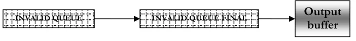
The various paths for the two kinds of instructions were devised in the manner shown so as to be cycle accurate with the DUV operation. Each valid instruction (ARITH/SHIFT) needs to be sent through the priority pipe (ARITH/SHIFT queues). The other stages are added to implement cycle accuracy and do appropriate priority checks and make dispatch decisions. The Input Buffer receives the instructions that are driven into the DUV by the Stimulus. Figure 4.6 shows the information content at each stage.
Figure 4.6 Information content at each stage
INVALID QUEUE INVALID QUEUE FINAL Output
buffer QUEUE Global table Port ID Tag INPUT BUFFER
Port ID (X) Command (reqX_cmd) Tag (reqX_tag) D1 (reqX_d1) D2(reqX_d2) R1(reqX_r1) Hold table Port ID Command Tag D1 D2 R1 TEMP Port ID Tag RAW Port ID Command Tag D1 D2 R1 OUTPUT BUFFER Tag INVALID QUEUE Port ID Tag
INVALID QUEUE FINAL
The input buffer passes this information to the Queue (Arith/Shift) based on the type of command the instruction holds. The information of the instruction is used in the hold and global tables to implement the priority scheme and decide the dispatching mechanism (toggling). After determining which item (instructions) can be dispatched from both the Arith queue and the Shift queue the eligible ones from both these queues are sent to the
Temp stage where again the port ID comparison will decide on whether to invoke the toggling mechanism or not. Although the global and hold table exist to prevent the data dependency hazards, a command that has left the global table needs to still be compared with an incoming instruction to prevent even such a rare occurrence of the data dependency. Hence the item that is leaving now needs to be added to the Raw stage so that data dependency checks later can be made. This also facilitates to provide the cycle accurate behavior of the environment.
The invalids as per the specification are sent directly to an output buffer and are output only when no other ARITH/SHIFT instruction is output during that cycle. The Invalid Queue acts as the input buffer for the invalid inputs. It contains just the Tag and Port ID information which is sufficient to detect any priority violations. The Invalid Queue Final
stage is similar to the Invalid Queue stage but it is a waiting stage for the invalid items incase there are valid items to be output (according to the design specifications invalids cannot be output if there are valid instructions waiting at the output buffer). When the output buffer is free of valid items this queue is checked and the invalid is sent to the output stage for comparison with the DUV output.
Following is a description of the vital methods or functions used in the Checker model.
take over. Once the inputs are sent to the queue the input buffer is cleared and awaits the next instruction. After updating the hold table and global table, based on a certain set of
clear and valid flags that are used in the implementation of the GTG algorithm, the instructions are held in the tables until they are good to go. The top most instruction of the global table that is good to go is moved to the temp stage. This is the portion of the function where the port contention i.e. one instruction each from both the queues having the same port ID is resolved. Once they are ready to be dispatched the dispatch()
function takes over the dispatch decisions part of this method. Once the dispatch is made and the instructions are added to the RAW stage, this method sees through that it is added to the output buffer and the flags set on instructions held in the hold table due to this data dependency are cleared. If there is nothing to send to the output buffer the invalid final queue is checked and its output is sent to the output buffer.
dispatch() is a method that is used to make the dispatch decisions after the instructions which are good-to-go are decided by the collaborative effort of the hold table and global table functions. The dispatch function is actually of two types: arith_dispatch() and
shift_dispatch(). They are chosen based on the port IDs of the top most instructions in both the queues that are good-to-go. If the port IDs are different then both the functions are called else if there is a port contention then either one of them is called based on a toggle bit (res_cont). To start with the preference is given to the arith_dispatch() and then the priority toggles. During the dispatch the valid bits in the hold table are cleared (using reset_valid())so that incoming instructions can take up its place in the hold table. The instruction is sent to the RAW stage.
Table 4.1 Environment Hold table
Every valid incoming instruction is added to the hold table after comparison with the rest to set the GTG attributes. A GTG valid is set if there is any conflict between the registers used by the instructions existing in the hold table and all registers in the incoming instruction. Useful registers vary on command basis as shown in the table below.
Command Useful Registers
ADD/SUB/SL/SR D1/D2/R1
FETCH/BEZ D1
BEQ D1/D2
STORE R1
Table 4.2 Useful Registers for each command
So if the incoming instruction is a STORE then the D1/D2/R1 of this instruction is compared with the useful registers of the instructions stored in the hold table to determine what to set the GTG values to. If there is any such conflict the tag value is stored so that this GTG can be cleared once the appropriate blocking instruction has been dispatched.
The fields in the hold table abide by the following rules:
1. When an incoming instruction has register conflicts with the items in the hold table a GTG valid is set. Under such conditions the tag value of the blocking instruction is stored in the GTG_tag attribute location.
GTG1 GTG2 GTG3 skip Branch
depend tag D1 D2 R1 valid cmd
valid tag raw valid tag raw valid tag raw valid tag 00
01 10
2. GTG valids are released and initialized back to zero once the instruction that has been blocking it has been dispatched.
3. GTGs are set in ascending order. First GTG1 then GTG2 and finally GTG3. Upon clearing up of the GTGs there is no precedence since the order in the hold table does not necessarily mean the order of dispatch.
4. GTG raw is set only when the incoming instruction has a RAW conflict with a hold table instruction else it is set to zero.
5. When an incoming instruction enters the queue after a previous branch instruction from the same port (indicated by a flag block) and the branch instruction hasn’t been dispatched yet, then the skip fields of the incoming instructions are set and the branch tag value is stored.
6. The branch dependency stores the tag value of a prior branch instruction whether it is valid or not in the hold table. This field takes a value of 4 by default since tags take values from 0-3.
7. A GTG is also set for a branch instruction that has a tag similar to a previously dispatched branch whose following command (that is to be skipped) hasn’t been dispatched as yet. This prevents dependency on the wrong branch. The Branch dependency field is of primary importance in checking these values.
8. All the other fields are information fields and are added directly.
Incoming instructions that are branches have their tags stored temporarily and set a block
flag high so that its following command may be traced.
global_table_funct() is a method used to implement the global table add values to the priority queue. The global table implementation has the following fields:
ID Tag Valid Clear
Any valid instruction that enters the queue stage and added to the hold table is also added to the global table. The ID and tag are informational fields that are added directly. The valid field is set only if the GTG valids or skip valid in the hold table for this instruction has been set. Clear is initially set to zero. If the valid field is zero then the instruction is compared with the item in the RAW stage and the valid is set to 1 and clear to 2 if there is a RAW conflict. If there is no RAW conflict then the valid remains to be zero. Valids with clear of value 2 are reset to zero in the next cycle. Once all the fields in the global table are set then the command is added to the priority queue (arith_prio or shift_prio).
match_priority() is a time consuming method executing every rise edge of the clock to compare the tags produced on the output and there by verify the priority of the instructions. Presence of stray tags or mismatch of tags at the output is reported as a DUV error.
run() is also function invokes the two primary TCMs, match_priority() and
gen_priority() of which all the others are sub-methods.
4.4.5 Coverage information
Functional coverage has been implemented using Specman’s Functional Coverage feature. Coverage has been implemented in this environment to cover inputs. Whenever the stimulator drives input signals on the DUV inputs, it emits an event on which coverage is triggered. On this event, the input command, the source registers and the destination register, the tag and the port are covered. Similarly cross-coverage is performed between various inputs and also between inputs and outputs.
that all tags have seen port clashes in all ports and all ports have been tested for the port clash condition. Whenever a port clash condition occurs, an event is emitted and the port and the tag are covered on this event. Coverage is also performed on the priority queue to determine how much of the queue is filled. The following section describes the various coverage points considered.
4.4.5.1 Coverage points
The various coverage points taken into consideration to stress the DUV to the maximum limit have been described here. These involve Value Coverage, Crosses and Transitions.
1. Value Coverage: Inputs are covered to ensure that it takes all its possible values.
a. Commands: To see if all possible commands have been covered. Testcase specifies all commands for the reqX_cmd and it is run for 5000 cycles.
b. Tag: Covered to check if all possible values have been utilized by the tag input. Testcase is run for 5000 cycles.
c. D1 register: Since this is dynamic partitioning, it takes really long to determine if D1 register has covered its entire range from 0-15. D1 must have had all register values atleast once.
d. D2 register: Since this is dynamic partitioning, it takes really long to determine if D2 register has covered its entire range from 0-15. D2 must have had all register values atleast once.
2. Cross Coverage: These are basic crosses to ensure critical combinations of inputs occur. Table 4.4 lists the various basic crosses performed.
Commands Tags D1 D2 R1 Data PortID
Commands - X X X X X X
Tags X - X X X - X
D1 X X - - - - X
D2 X X - - - - X
R1 X X - - - - X
Data X - - - X
PortID X X X X X X X
Table 4.4 Cross Coverage
a. Commands
i. Tag: Covered to ensure all commands were associated with all tags.
ii. D1: Covered to ensure all commands were associated with all D1 register values atleast once.
iii. D2: Covered to ensure all commands were associated with all D2 register values atleast once.
iv. R1: Covered to ensure all commands were associated with all R1 register values atleast once.
v. Data: STORE commands with data values closer to FFFFFFFF are covered to ensure overflows.
vi. PortID: Covered to ensure all Ports have all types of commands.
b. Tags
ii. D1: Covered to ensure all possible combinations of D1s and tags were covered.
iii. D2: Covered to ensure all possible combinations of D2s and tags were covered.
iv. R1: Covered to ensure all possible combinations of R1s and tags were covered.
v. PortID: Covered to ensure all Ports have all types of tags.
c. D1
i. Commands: Covered to ensure all commands were associated with all D1 register values atleast once.
ii. Tag: Covered to ensure all possible combinations of D1s and tags were covered.
iii. Port ID: Covered to ensure all Ports have all types of D1s atleast once.
d. D2
i. Commands: Covered to ensure all commands were associated with all D2 register values atleast once.
ii. Tag: Covered to ensure all possible combinations of D2s and tags were covered.
iii. Port ID: Covered to ensure all Ports have all types of D2s atleast once.
e. R1
i. Commands: Covered to ensure all commands were associated with all R1 register values atleast once.
ii. Tag: Covered to ensure all possible combinations of R1s and tags were covered.
f. Data
i. Commands: STORE commands with data values closer to FFFFFFFF are covered to ensure overflows.
g. PortID: This is covered with all inputs to make sure that it has every combination of inputs associated with every port.
3. Additional Crosses: These ensure that most of the possible combinations of inputs and outputs do occur in atleast one or more transactions. Table 4.5 lists these special crosses.
Output Response Port Clashes
Commands X -
Tags X X
PortID - X
Table 4.5 Additional Cross Coverage
a. Commands
Output Response: Covered to ensure that all commands have been matched to all possible output responses (1,2 and 3). It is particularly interesting to note that by covering that all commands get a response of 3, we are implicitly covering the case of all commands following a taken branch.
b. Tags