Reconfigurable kinematics, dynamics and control process for industrial robots.

University of Windsor University of Windsor

Scholarship at UWindsor

Scholarship at UWindsor

Electronic Theses and Dissertations Theses, Dissertations, and Major Papers

1-1-2007

Reconfigurable kinematics, dynamics and control process for

Reconfigurable kinematics, dynamics and control process for

industrial robots.

industrial robots.

Ana Djuric

University of Windsor

Follow this and additional works at: https://scholar.uwindsor.ca/etd

Recommended Citation Recommended Citation

Djuric, Ana, "Reconfigurable kinematics, dynamics and control process for industrial robots." (2007). Electronic Theses and Dissertations. 7222.

https://scholar.uwindsor.ca/etd/7222

RECONFIGURABLE KINEMATICS, DYNAMICS AND

CONTROL PROCESS FOR INDUSTRIAL ROBOTS

by

Ana Djuric

Dissertation

Submitted to the Faculty of Graduate Studies through

Mechanical, Automotive, and Materials Engineering in Partial Fulfillment of the Requirements for

the Degree of Doctor of Philosophy at the University of Windsor

Windsor, Ontario, Canada 2007

1*1

Library and Archives Canada Published Heritage Branch

395 Wellington Street Ottawa ON K1A0N4 Canada

Bibliotheque et Archives Canada Direction du

Patrimoine de I'edition

395, rue Wellington Ottawa ON K1A0N4 Canada

Your file Votre reference ISBN: 978-0-494-42379-0 Our file Notre reference ISBN: 978-0-494-42379-0

NO TICE:

The author has granted a non­ exclusive license allowing Library and A rchives C anada to reproduce, publish, archive, preserve, conserve, com m unicate to the public by

telecom m unication or on the Internet, loan, distribute and sell theses

w orldw ide, fo r com m ercial or non­ com m ercial purposes, in m icroform , paper, electronic and/o r any other form ats.

AVIS:

L'auteur a accorde une licence non exclusive perm ettant a la Bibliotheque et A rchives C anada de reproduire, publier, archiver,

sauvegarder, conserver, transm ettre au public par telecom m unication ou par Nntem et, preter, distrib ue r et vendre des theses partout dans le monde, a des fins com m erciales ou autres, sur support m icroform e, papier, electronique et/ou autres form ats.

The author retains copyright ow nership and m oral rights in this thesis. N either the thesis

nor substantial extracts from it m ay be printed or otherw ise reproduced w ith o u t the author's perm ission.

L'auteur conserve la propriete du droit d'auteur et des droits m oraux qui protege cette these. Ni la these ni des extraits substantiels de celle-ci ne doivent etre im prim es ou autrem ent reproduits sans son autorisation.

In com pliance w ith the C anadian Privacy A ct som e supporting form s may have been rem oved from this thesis.

W hile these form s m ay be included in the docum ent page count,

the ir rem oval does not represent any loss of content from the

C onform em ent a la loi canadienne sur la protection de la vie privee, quelques form ulaires secondaires ont ete enleves de cette these.

ABSTRACT

This work, aims at developing a highly reconfigurable control system which intelligently unifies the reconfiguration and manages the interaction of individual robotics control systems within a reconfigurable manufacturing system (RMS). For performing any reconfigurable control process, a reconfigurable plant model that represents different robotic systems was developed.

Instead of modeling and creating new reconfigurable systems, new modular robots and machines, the existing systems, robots and machines were defined as reconfigurable systems, modular robots and machines according to their reconfigurable aspects. From the study of existing robotic software and reviewing the literature, the idea of grouping robots according to their kinematic similarities was conceived and the Reconfigurable PUMA-Fanuc (RPF) model was developed.

A generic solution module called the Unified Kinematic Modeler and Solver (UKMS) implements the geometric approach for solving the inverse kinematic problem for the (RPF) model.

A Reconfigurable PUMA-Fanuc Jacobian Matrix (RPFJM) and reduced Reconfigurable PUMA-Fanuc Singularity Matrix (RPFSM) were developed.

The Reconfigurable Robot Workspace (RRW) was developed using the Filtering Boundary Points (FBP) method.

For the symbolic calculation of the RPF dynamics equations, named Reconfigurable PUMA-Fanuc Dynamic Model (RPFDM), the recursive Newton- Euler algorithm was employed, using the symbolic algebra package MAPLE 10®. The simplification of the model was done using the Automatic Separation Method (ASM). The significance of the RPFDM is that it automatically generates each element of the inertia matrix A, Coriolis torques matrix B, centrifugal torques

matrix C, and gravity torques vectors G. This model was extended to include the robot actuator dynamics and the complete electro-mechanical model named RPFDM+ is presented.

The Reconfigurable Control Platform (RCP) was developed using Matlab/Simulink® software. As a case study, the PUMA 560 robot was selected and the reconfigurable “PI” controller was designed as a function of the motor parameters.

All eight modules (RPF, UKMS, RPGJM, RPFSM, RRW, RPFDM, RPFDM+, and RCP) can be reconfigured by changing the parameters K l , K 2, K 2, K 4, K 5,

DEDICATION

ACKNOWLEDGEMENTS

I would like to express my sincerest and deepest appreciation to my supervisor Professor Waguih ElMaraghy for giving me the opportunity, his guidance, and for helping me throughout the course of my Ph.D program. I would also like to extend my thanks to my Supervisory Committee, Dr. Waguih ElMaraghy, Dr. Robert Gaspar, Dr. Bruce Minaker, Dr. Nader Zamani, and Dr. Jonathan Wu, for their comments and time in reviewing my dissertation.

I would like to acknowledge the great help and insight that I received from the IMS Centre directors, Professor Hoda ElMaraghy and Professor Waguih ElMaraghy, for giving me the chance to discuss the research topics with other members through the regular meetings they arranged for us. I learned a lot from these meetings. I would like to extend my thanks to all other members in IMS Centre especially to Dr. R. Jill Urbanic, Biljana Marinkovic and my college Dr. Mirjana Filipovic for their suggestions and encouragement.

I would like to thank the Staff of both, the Department of Mechanical, Materials and Automotive Engineering and Industrial and Manufacturing Systems Engineering Department: Ms. Jacquie Mummery, Mr. Ram Barakat, Ms. Zaina Batal, and Ms. Rosemarie Gignac and Ms. Barbara Denomey for their support and kind assistance during my study.

TABLE OF CONTENTS

A B S T R A C T ...I l l

D E D IC A T IO N ...V

A C K N O W L E D G E M E N T S ... V I

LIST O F T A B L E S ... X I

LIST O F F IG U R E S ... X I I I

N O M E N C L A T U R E ...X V I I I

A b b re v ia tio n s ...x v i i i

Sy m b o l s...x x

1. IN T R O D U C T IO N ...1

1.1. Problem St a t e m e n t...11

1.2. Ba c k g r o u n do f Ro b o t ic s... 12

1.2.1. Description o f a Robot M odel...13

1.2.2. Robot Geometry....15

1.2.3. Fundamentals o f Robot Kinematics...17

1.3. Re sea r c h Ap p r o a c h... 21

2. G E N E R A L IZ E D R E C O N F IG U R A B L E 6 - J O IN T R O B O T M O D E L IN G ... 23

2.1. In t r o d u c t io nt o Un ifie d Re c o n fig u r a b l e Open Co n tr o l Ar c h it e c t u r e (UROCA)23 2.2. Rec o n fig u r a b l e As p e c t so f In d u str ia l Ro b o tic Sy s t e m s...24

2.3. De v e l o p m e n to ft h e R PF Mo d e l...26

2.3.1. The Design o f Configuration Parameters K t...28

2.4. A Un ified Ge o m e t r y-Ba s e d So l u t io n... 39

2.4.1. Arm Solution for the First Three Joints ... 41

2.4.2. Arm Solution for the Last Three Joints...49

2.5. Sim ulation Re su ltsa n d Dis c u s s io n s... 55

3. SINGULARITY ANALYSIS OF A RECONFIGURABLE PUMA -FANUC ROBOTIC MODEL VIA A RECONFIGURABLE JACOBIAN MATRIX APPROACH...66

3.1. Re c o n fig u r a b le PU M A -Fa n u c Ja co b ia n Ma t r ix (R P F JM )... 66

3.1.1. Example o f PUMA Jacobian M atrix...69

3.1.2. Example o f Fanuc Matrix...70

3.2. Re d u c e d Re c o n fig u r a b l e P U M A -Fa n u c Sin g u la r ity Ma t r ix (R P F S M )... 71

3.2.1. Forearm Singularity o f the RPF Model...73

3.2.2. Wrist Singularity o f the RPF Model...74

3.2.3. Example o f PUMA Reduced Singularity Matrix...75

3.2.4. Example o f Fanuc Reduced Singularity Matrix...75

4. ROBOT WORK ENVELOPE...76

4.1. Ca lc ulatio no f Re c o n fig u r a b l e Ro b o t Wo r k s p a c e (R R W )... 76

4 .2. Filter in g Bo u n d a r y Po in t s (FB P) Me t h o d...78

4.2.1. Envelope for the ABB IRB 1400 robot...81

4.2.2. Envelope for the Fanuc ARC Mate 120iL robot...81

5. GENERALIZED RECONFIGURABLE 6 - JOINT ROBOT DYNAMICS... 82

5.1. Desc r iptio n o ft h e R P F D M ...82

5.2.1. Forward Computation o f Velocity and Accelerations...86

5.2.2. Backward Computation o f Forces and Moments...88

5.3. A u to m atic S e p a ra tio n M e th o d (ASM )...89

5.4. Co u p lin g Mo to r Dy n a m ic sw it h Link Dy n a m ic s... 92

5.5. Exa m pleo f So m e Ma t r ix Ele m e n t s fo rth e R PFD M a nd PU M A 5 6 0 ... 95

6. RECONFIGURABLE CONTROL PLATFORM FOR PUMA 560 ROBOT... 100

6.1. DC Mo t o r Sizing Pr o c e d u r e... 100

6.2. DC Mo t o r Rec o n fig u r a b l e Po s it io n Co n tr o l De s ig n... 113

6.3. Im p l e m e n t in g DC Mo t o r Re c o n fig u r a b l e Po s it io n Co n t r o l l e rf o r P U M A 560 Ro b o t...124

6.4. Pr o c e d u r e f o r Re p r e s e n t in g Ro b o ts u sin gall Six Re c o n fig u r a b l e Mo d u le s ..132

7. FUTURE WORK...134

8. CONCLUSIONS...139

REFERENCES...143

APPENDIX A: REDUCED RPFJM EQUATIONS...155

APPENDIX B: REDUCED RPJM EQUATIONS... 158

APPENDIX C: REDUCED RFJM EQUATIONS... 160

APPENDIX D: REDUCED RECONFIGURABLE PUMA -FANUC SINGULARITY MATRIX (RPFSM)... 162

APPENDIX E: REDUCED RECONFIGURABLE PUMA SINGULARITY M ATRIX... 165

APPENDIX F: REDUCED RECONFIGURABLE FANUC SINGULARITY M ATRIX...167

APPENDIX G: REDUCED RECONFIGURABLE PUMA 560 DYNAMIC PARAMETERS ..169

VITA AUCTORIS... 176

LIST OF TABLES

Table 1.1: Lite r a tu r e Re v ie w Su m m a r y Ma t r ix... 8

Table 2.1: Kin em a ticty p ecla ss ific a tio no f r o b o tics y s t e m sfrom 11 d if f e r e n t m a n u f a c t u r e r s... 27

Table 2.2: D-H pa r a m ete r s fo r PU M A -like Table 2.3: D-H p a r a m ete r sfo r Fa n u c-like 36 T a b le 2.4: D-H p a ra m e te rs f o r th e RPF m o d el...38

Table 2.5: Po ssiblea r m c o n f ig u r a t io n sf o r Jo in t 2 (Lee C. S. G„ a n d Zieg le r M., 1 9 8 4 )... 46

T a b le 2.6: Arm c o n fig u ra tio n s f o r PUMA ty p e r o b o t s ...49

Table 2.7: Armc o n f ig u r a t io n sf o r Fa n u ct y p er o b o t s... 49

Table 2.8: Va r io u so r ie n t a t io n sfo rt h ew r is t...50

T a b le 2.9: V a rio u s p o ints on th e ABB IR B 1400 r o b o t P a t h ...58

Table 2.10: Jo in ts o l u t io n sfo r p o in t 2 ... 60

Table 2.11: Jo in ts o l u t io n sfo r p o in t 3 ... 60

Table 2.12: Jo in ts o l u t io n sfo r p o in t 4 ... 60

Table 2.13: Jo in ts o l u t io n sfo r p o in t 5 ... 60

Table 2.14: Jo in ts o l u t io n sfo rp o in t 6 ... 61

Table 2.15: Va r io u sp o in t so nth e A R C Ma t e120iL r o b o t Pa t h... 62

Table 2.16: Jo in ts o l u t io n sfo rp o in t 2 ... 64

Table 2.17: Jo in ts o l u t io n sf o rp o in t 3 ... 64

Table 2.18: Jo in ts o l u t io n sfo r p o in t 4 ... 64

Ta b l e2.20: Jo i n t s o l u t io n s f o rp o i n t 6... 65

Ta b l e 6.1: PUMA 560 DC m o t o r s i n f o r m a t i o n...106

LIST OF FIGURES

Fig u r e 1.1: Po la r, Cy l in d r ic a l, Ca r t e s ia n, Jo in t e d Ar m, S C A R A ... 15

Fig u r e 1.2: To o land Ba s e fr a m esfo rt h e PU M A 5 60 r o b o t... 16

Fig u r e 1.3: Thelo w erpa irj o in t s... 17

F ig u re 1.4: C o o rd in a te fram e s and D-H p a r a m e te rs ... 20

Fig u r e 2.1: U R O C A Ar c h it e c t u r e... 23

Fig u r e 2.2: Cla ssific a tio no f Indu str ia lr o b o t s... 25

Fig u r e 2.3: Fa n u c-t y p ea n d PU M A -ty per o b o tsa n dt h e irjo in tt h r e ed ir e c t io n s...26

Fig u r e 2.4: Co m p a r is o n b e tw een PU M A -Fa n u ct y p eo fr o b o tsa n do th e rr o b o t s...28

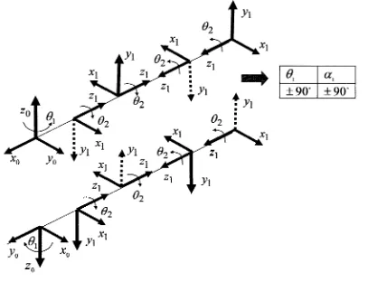
Fig u r e 2.5: Relationb e tw e e n d ir e c tio n s o f Jo in t 1 a n d Jo in t 2 ... 29

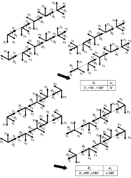
Fig u r e 2.6: Relationb e tw e e n d ir e c tio n so f Jo in t 2 a n d Jo in t 3 ... 30

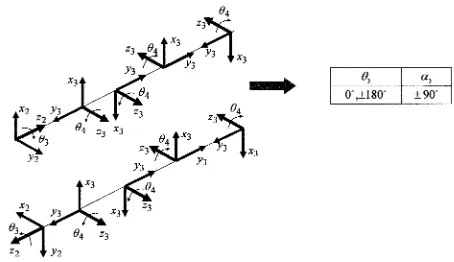
Fig u r e 2.7: Relation b e tw e e n d ir e c tio n s o f Jo in t 3 a nd Jo in t 4 ... 31

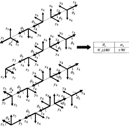
Fig u r e 2.8: Relation b e tw e e n d ir e c t io n so f Jo in t 4 a n d Jo in t 5 ... 32

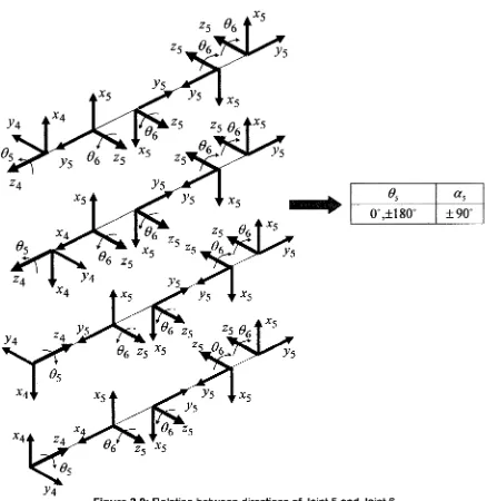
Fig u r e 2.9: Relation b e tw e e n d ir e c tio n so f Jo in t 5 a n d Jo in t 6 ... 33

Fig u r e 2.10: Relationb e tw eend ir e c t io n so f Jo in t 6 a nda p p r o a c hv e c t o r...34

Fig u r e 2.11: Gen e r ic P U M A k in em a ticm o d e l...35

Fig u r e 2.12: Gen e r ic PU M A k inem aticm o d e l...36

Fig u r e 2.13: RPF k in e m a t icm o d e l... 37

Fig u r e 2.14. De f in it io no fv a r io u sa rmc o n f ig u r a t io n s... 39

Fig u r e 2.15: Po s it io nv e c t o rpfo rsph er ic a lw r is tr o b o t s...41

Fig u re 2.16: LA (L e f t A rm ) p ro je c tio n s o f th e position v e c t o r p o n to th e x 0j 0 p la n e 42

Fig u r e 2.17: RA (Rig h t Ar m) p r o je c t io n so ft h e p o s it io nv e c t o r p o n t ot h e x 0y 0p l a n e... 43

Fig u r e 2.18: Pr o jec tio n softh ep o s it io nv e c t o r p o n t ot h e x 1y 1p l a n e...45

Fig u r e 2.19: Fo u rc o m b in a tio n so f A a n d E c o n f ig u r a t io n s f o rj o in t 2 s o l u t io n... 45

Fig u r e 2.20: Jo in t 3 ang lefo r P U M A g r o u p...47

Fig u r e 2.21: Jo in t 3 an g lefo r Fa n u cg r o u p...47

Fig u r e 2.22: Jo in t 4 an g lefo r P U M A a nd Fa n u cg r o u p s... 51

Fig u r e 2.23: So lu tio n f o r Jo in t 5 (PU M A an d Fa n u cg r o u p s r e s p e c t iv e l y)... 53

Fig u r e 2.24: So lu tio n fo r Jo in t 6 ...54

Fig u r e 2.25: Th r e em a jo rstep s f o rr e p r e s e n t in g t h ek in em a tic sm o d e lo far o b o tin U R O C A ...57

Fig u r e 2.26: Fa n u c ABB IRB 1400 w it h p o in t so n t h epatha nd its D-H p a r a m e t e r s...58

Fig u r e 2.27: Jo in ts o l u tio n sf o rp o in t 1 ... 59

F ig u re 2.28: Fanuc A R C M ate120iL w ith points on th e path and its D-H p a ra m e te rs ... 61

Fig u r e 2.29: Jo in ts o l u tio n sf o rp o in t 1 ...63

Fig u r e 3.1: Po s it io nv e c t o r p Ef o rsph er ic a lw r is tr o b o t s... 72

Fig u r e 4.1: En v e lo p e Bo u n d a r yf o r Jo in t 2 a nd Jo in t 3 IR B 6400-24 (Wo r k s p a c e 4 ® s o f t w a r e) ...77

Fig u r e 4.2: Bo u n d a r ya n d In t e r io rp o in t s... 78

Fig u r e 4.3: Sidev ie wo fth ea r e aa r o u n dth e Pi p o in tint h e Ro b o t Wo r k s p a c e... 79

Fig u r e 4.4: To pv ie wo ft h ea r e aa r o u n dth e Pi p o in t int h e r o b o tw o r k s p a c e...79

Fig u r e 4 .5 :2 -3 e n v elo p eand 1 -2-3 e n v e l o p e...80

Fig ure 4 .7 :2 -3 en v elo p ea n d 1-2-3 e n v elo p efo rth e Fa n u c A R C Ma te 120iL r o b o t... 81

Fig u r e 5.1: Ge n e r ic PU M A -Fa n u c Dy n a m ic Mo d el (R P F D M )... 83

Fig u r e 5.2: Fo r w a r da n d Ba ck w ard Dy n a m ic Fl o w c h a r t... 85

Fig ure 5.3: Lu m pe dm o d e lo flinkw it h DC Mo to ra n dg e a r... 93

Fig ure 5.4: PU M A 560 DH p a r a m e t e r s... 95

Fig ure 5.5: PU M A 560 DH linkm a ssv a l u e... 95

Fig ure 6.1: DC m o to r blockd ia g r a m...101

Fig u r e 6.2: DC m o to r 1 s p e e d-t o r q u ec u r v e... 103

Fig ure 6.3: To r q u e linesfo rd if f e r e n tvo l ta g es (DC m o t o r 1 ) ... 103

Fig ure 6.4: Cu r r e n t Line (D C m o to r 1 ) ... 104

Fig ure 6.5: Po w e rc u r v e (DC m o to r 1 ) ... 105

Fig ure 6.6: Ef f ic ie n c yc u r v e (DC m o t o r 1 )...105

Fig ure 6.7: DC m o to r 1 c h a r a c t e r is t ic s... 107

Fig u r e 6.8: DC m o to r 2 c h a r a c t e r is t ic s... 107

Fig u r e 6.9: DC m o t o r 3 c h a r a c t e r is t ic s... 108

Fig u r e 6.10: DC m o to r 4 c h a r a c t e r is t ic s... 108

Fig u r e 6.11: DC m o t o r 5 c h a r a c t e r is t ic s... 109

Fig u r e 6.12: DC m o t o r 6 c h a r a c t e r is t ic s... 109

Fig ure 6.13: Mo t o r 1 v e l o c it yd y n a m ic s, r o o tl o c u s... 110

Fig ure 6.14: Mo t o r 2 v e l o c it yd y n a m ic s, r o o tl o c u s... 111

Fig ure 6.15: Mo t o r 3 v e l o c it yd y n a m ic s, r o o tl o c u s... 111

Fig u r e 6.17: Mo t o r 5 v e l o c it yd y n a m ic s, r o o tl o c u s...112

Fig ure 6.18: Mo t o r 6 v e l o c it yd y n a m ic s, r o o tl o c u s... 113

Fig ure 6.19: Mo t o r 1: Ro o tlo c u so fp o s itio nc o n t r o ls y s t e m...114

Fig ure 6.20: Mo t o r 1: m a g n if ie d - polesa r o u n dz e r o...114

Fig ure 6.21: Mo t o r 1: Ro o tlo cuso ft h ep o s it io nc o n tr o ls y s t e mw it hana d d e dz e r o 115 Fig ure 6.22: Mo t o r 2: Ro o tlo c u so fp o s it io nc o n t r o ls y s t e m... 115

Fig ure 6.23: Mo t o r 2: m a g n if ie d - p olesa r o u n dz e r o...116

Fig u r e 6.24: Mo t o r 2: Ro o tlo c u so ft h ep o s it io n c o n t r o ls y s t e mw it h a d d e daz e r o 116 Fig ure 6.25: Mo t o r 3: Ro o tlo c u so fp o s it io n c o n t r o ls y s t e m... 117

Fig ure 6.26: Mo t o r 3: m a g n if ie d - polesa r o u n dz e r o...117

Fig ure 6.27: Mo t o r 3: Ro o tlocuso fth ep o s it io n c o n tr o ls y s t e m w it hana d d e dz e r o... 118

Fig ure 6.28: Mo t o r 4: Ro o tlocuso fp o s it io n c o n t r o ls y s t e m... 118

Fig ure 6.29: Mo t o r 4: m a g n if ie d - polesa r o u n dz e r o...119

Fig ure 6.30: Mo t o r 4: Ro o tlo cusofth e p o s it io n c o n tr o ls y s t e mw it hana d d e dz e r o... 119

Fig ure 6.31: Mo t o r 5: Ro o t lo cusofp o s it io nc o n t r o ls y s t e m... 120

Fig ure 6.32: Mo t o r 5: m a g n if ie d - polesa r o u n dz e r o...120

Fig ure 6.33: Mo t o r 5: Ro o tlo cuso ft h e p o s it io n c o n tr o ls y s t e mw itha d d e daz e r o...121

Fig ure 6.34: Mo t o r 6: Ro o tlo cuso fp o s it io nc o n t r o ls y s t e m... 121

Fig ure 6.35: Mo t o r 6: m a g n if ie d- polesa r o u n dz e r o...122

Fig u r e 6.36: Mo t o r 6: Ro o tlo c u so ft h e p o s it io nc o n tr o ls y s t e m w it hana d d e dz e r o... 122

F ig u re 6.37: PI c o n t r o l l e r f o r th e DC M o t o r 1 ... 123

F ig u re 6.39: Schem atic diagram o f th e PUMA 560 r o b o t f i r s t l i n k ...126

Fig u r e 6.40: Sc h em a ticdia g r a m ofth ef ir s tlinkd y n a m ic sa ndf ir s t m o t o rd y n a m ic s 127 F ig u re 6.41: Schem atic diagram o f th e C o n t r o l l e r w ith input com m and...128

F ig u re 6.42: Schem atic diagram o f th e PI C o n t r o l l e r ...128

F ig u re 6.43: Schem atic diagram o f th e e le c t r ic a l p a r t o f th e DC m o t o r ...128

F ig u re 6.44: Schem atic diagram o f th e PUMA 560 r o b o t ...129

F ig u re 6.45: PUMA 560 r o b o t p ath in UROCA s o f t w a r e ... 130 F ig u re 6.46: The resp o n se o f th e PUMA 560 jo in t positions using th e PI r e c o n fig u r a b le CO NTROLLER...... 131

Fig u r e 6.47: Auto m a tic r o b o tplanta n dc o n t r o l g e n er a tio nu s in gm a nualin p u to f dyna m ic e q u a t io n s...133

Fig u r e 7.1: Ro bo to f f s e tw r is t... 134

Fig u r e 7.2: Au to m a ticr o b o tplanta ndc o n t r o lg e n er a tio nu s in g Blo ck Bu il d e rfo r Sim u l in k... 137

NOMENCLATURE

Abbreviations

A:

Arm.

ASP:

Automatic Separation Procedure.

AA:

Above arm.

BA:

Below arm.

D:

Down.

DD:

Dynamic Damping.

DF:

Do not flip.

D-H:

Denavit - Hartenberg.

DOF:

Degree of Freedom.

E:

Elbow.

EA:

Elbow Above.

EB:

Elbow Below.

F:

Flip.

FBP:

Filtering Boundary Points.

HIC:

Hybrid Impedance Control.

LA:

Left Arm.

L&B:

Left and Below.

NSERC:

Natural Science and Engineering Council of Canada.

OOP:

Objected Oriented Programming.

PD:

Proportional Differential.

PI:

Proportional Integral.

PID:

Proportional Integral Differential.

PUMA:

Programmable Universal Machine for Assembly.

RA:

Right arm.

R&A:

Right and Above.

R&B:

Right and Below.

RCP:

Reconfigurable Control Platform.

RMS:

Reconfigurable Manufacturing System.

RPF:

Reconfigurable Puma-Fanuc.

RPFJM:

Reconfigurable Puma-Fanuc Jacobian Matrix.

RPFSM:

Reconfigurable Puma-Fanuc Singularity Matrix.

RRW:

Reconfigurable Robot Workspace.

RPFDM:

Reconfigurable Puma-Fanuc Dynamic Model.

RPFDM+:

Reconfigurable Puma-Fanuc Dynamic Model Plus.

RRP:

SCARA:

U:

UKMS:

UROCA:

W:

WD:

WU:

Symbols

A :

A :

a:

at .

a i j

-Reconfigurable Robot Platform.

Selective Compliant Articulated Robot Arm.

Up.

Unified Kinematic Modeler and Solver.

Unified Reconfigurable Open Control Architecture.

Wrist.

Wrist down.

Wrist up.

6 x 6 Inertia matrix.

Diagonal matrix.

Approach vector

i ,h Link offset.

Matrix A elements.

'(% ):

'(V,):

ith Linear acceleration.

ith Linear acceleration of the center of mass.

B \

b

l

-6x15 Coriolis torques matrix.

Load Damping Coefficient.

B

: Diagonal matrix.

bUj: Matrix B elements.

C: 6x 6 Centrifugal torques matrix.

C : Diagonal matrix.

Cb : Boundary singularities.

C; : Interior singularities.

Cy: Matrix C elements.

dt : i th Link length.

E: Center of the end-effector.

Eg : Back electromotive force.

e: Efficiency.

'( / * ) : Joint forces.

6 CfTool) = 0: End-effector force.

G: 6x1 Gravity torques vector.

' g : ith Gravity vector.

It : i th Moment of inertia about center of mass of each link.

im: Armature current.

J

: The Jacobian matrix.

J n: 3x3 block of the Jacobian matrix.

J2 2 ■ 3x3 block of the Jacobian matrix.

J E : End-effector Jacobian matrix.

J L: Load Inertia.

J m\ Armature Inertia.

J w: Wrist Jacobian matrix.

K b: Voltage constant.

K f : i ,h Configuration parameter of the ith twist angel a t .

K t : Torque constant.

L m : Armature Inductance.

M : Parameter.

mi: i th Link mass.

N : Gear ratio.

n: Normal vector.

'(« *): Joint moments.

Nl : Number of teeth of the output gear (load gear).

6 ( 6«7w ) = 0 : End-effector moment.

0 3, 0 4, 0 5,O6 : Centers of the 3th, 4 th, 5th and 6 th joints coordinate frames.

0 3x3: 3x3 zero matrix.

p : Position vector which points from the origin of the shoulder coordinate system ( x 0, y 0, z 0) to the point where the last three joints are intersecting.

p 6\ Position vector which points from the origin of the shoulder coordinate system ( xQ, y Q, z 0) to the position of the end-effector.

Pci: i th Radial distance to the center of mass of each link.

p E: Position vector of the end-effector center E .

PIN: Input power.

i~lPi: i th Position matrix.

Pt : Point on the 2-3 envelope

Pt i ,Pa ,Pn ,Pi4: Points in each quadrant of the local coordinate system.

POUT: Output power.

p x, p p z \ Coordinates of the position vector p with respect to the

( x 0, y 0, z 0) .

p w: Position vector of the spherical wrist W .

r - Vector o f joint velocities.

q: Vector of joint acceleration.

R P M: Rotation per Minute.

r : Parameter.

r, '■ Center of mass for \th link.

11R,: i th Rotational matrix.

C~ % )T: Transpose of all rotational matrices.

Rm '■ Armature Resistance.

S: Parameter.

s: Sliding vector.

Orf .

J6- Homogeneous transformation matrix, which specifies the

position and orientation of the end point of manipulator with respect to the base coordinate system.

i — \ r r > .

* i ' Homogeneous transformation matrix from (i - \)th link to i th link.

I'm '■ Motor generated torque.

T

s t a l l ' Stall Torque.

V : Armature Voltage.

Vmax: Maximum voltage.

w: Parameter.

W: Center of the spherical wrist.

XE : End-effector velocity.

Xw : Wrist velocity.

x j: Vector of generalized Cartesian coordinates.

: Vector of Cartesian velocities.

Xj: Vector of Cartesian acceleration.

z - w : Local coordinate system.

a i: i th Twist angle.

!(°a;): i th Angular acceleration.

P : Angle.

8 : Small distance from P..

(/>-. Angle.

<p: Angle.

9i : i th Joint angle.

O f: i th Joint angle for Right Arm configuration.

: ith Angular velocity vector.

6m: Angular position of armature.

t : Load torque.

Q : Parameter.

a): Angular velocity of armature.

i (°coi) : ith Angular velocity.

CHAPTER ONE

1. INTRODUCTION

A generic, reconfigurable kinematic module was an important need for the Unified Reconfigurable Control Architecture (UROCA) an architecture developed as part of the Strategic Research Project at the University of Windsor, supported by the Natural Science and Engineering Council of Canada (NSERC) Strategic Project Grant in “Reconfigurable Control Process for Manufacturing” provided to Prof. W. ElMaraghy.

Previous research investigations, for the sake of having several generic solutions, classified robot kinematic groups according to their twist angles, which are fixed for each group (Balkan M. T., et al., 2001). Accordingly, a different solution was provided for each group. The UKMS, unlike the others, accepts all the possible orientations for each joint within the RPF model, and therefore, it discards any classification that is based on having fixed twist angles. Instead, the UKMS unifies the model and generalizes the solution for robots of different twist angles rather than having different solutions for small groups of 6R robots with fixed twist angles.

Series was presented by Balkan M. T., et al., 2000. It is based on parameterised joint variables and analytical inverse kinematic solutions, which were proposed for some classes of robots according to a classification made by the authors. Bekir K. and Serkan A., 2000 have implemented the artificial neural-network approach for solving the inverse kinematics of one type of six-joint robot. The well-known fixed- point iteration algorithm for solving a non-linear system of equations was applied by Tourassis V. D. and Ang M. H. Jr, 1989 for solving the inverse kinematic problem of 6R robots. Manseur R. and Doty K. L. made a series of publications (Manseur R. and Doty K. L., 1996), (Manseur R. and Doty K. L., 1992), (Manseur R. and Doty K. L., 1989), (Manseur R. and Doty K. L., 1988) for solving the inverse kinematics of 6R manipulators by applying iterative and one-dimensional numerical approaches. A unified kinematic approach for solving robot kinematics has been applied on the PUMA 560 robot, (Gu Y. L. and Ho J. S., 1990).

The geometric approach for solving the inverse kinematic problem was applied for three-joint placeable robots with either rotational or translational joints by Fu H.,

et al., 1998. Fischer I.S., 2000 extended the geometric method for application to

the seven-joints Space Station Remote Manipulator System (SSRMS). Fu H., et al., 2000 have presented four new geometric invariants for the 6R manipulators in order to eliminate the joint variables in closure equations developed for solving this type of manipulator. These four invariants replace the Gaussian elimination process that was frequently used by other researchers. (Chapelle F., and Bidaud P., 2000) implemented an evolutionary symbolic regression algorithm for approximating the inverse kinematic model of any generic 6R manipulators. Her M.

G., et al., 2002 presented a paper that concerned the inverse kinematic

the RPF model for the moment. The RPF model will be extended in future to include this type of robot.

In this work, solving the inverse kinematic problem of the RPF model, which has the first three joints rotating and the last three joint axes intersecting at a point, is performed by the geometric approach (Lee C. S. G., and Ziegler M., 1984). This approach, as was more elaborated by Fu K.S., et al., 1987 and Owens J. P., 1994, is generalized for application to a wide class of 6R industrial robots that fall within the scope of our RPF model. Some modifications and adjustments made to the geometric approach were necessary in order to generalize it for application to the RPF model. In the first place, have chosen to implement this approach because it is much simpler than the other methods for application to different robotic systems having rotational joints. The resulting unified geometric-based solution can be used for any robotic manipulator that has a kinematic structure falling within the scope of the RPF model. The main feature of this solution is that one can use the same equations, which include newly introduced configuration parameters, for solving a wide variety of 6R kinematic groups in the RPF model.

Currently there is interest in research on the modeling and creation of reconfigurable systems, modular robots and machines (Matsumaru T., 1995), (Kelmar L. and Khosla P., 1988), (Benhabib B., et al., 1989), (Chen I. M. and Yang G., 1996), (Podhorodeski R. P. and Nokleby S. B., 2000). This work is based on the power of comparison between different robotic systems, and the result is the development of reconfigurable parameters for solving their inverse kinematics. Future research will extend the unified approach to reconfigurable robots.

A comparison, using three different methods for calculating, the Jacobian of 6 DOF robots with rotary or sliding joints are presented by Fu K.S., et al., 1987 and applied on the PUMA robot. By employing symbolic reduction techniques in conjunction with the separation of the resultant equations into on-line, temporary variables and off-line constraints, efficient formulations of the Jacobian, inverse Jacobian, and inverse Jacobian multiplied by a vector have been developed by Leathy M. B., et al., 1987. The Jacobian can be obtained by a simple method explained in (Spong M. W. and Vidyasagar M. 1989. The study and resolution of singularities for the PUMA robot were analyzed in detail by Cheng F. T., et al.,

1997, Oenny D., eta l., 2000, and Yuan J., 2001.

An important step for robot singularity analysis is task decoupling. This concept has been known since Pieper’s pioneering work (Pieper, D. L, 1968). The complete analysis of task decoupling was done in detail by Tourassis V. D. and Ang M. H. Jr, 1995.

The structural synthesis and the singularity analysis of six different families of orthogonal anthropomorphic robotic manipulators with 6R degrees of freedom, were presented by Gogu G., 2002. The kinematics singularities of each family were analyzed and interpreted both algebraically and geometrically. The singular configurations of 6R robots with spherical wrist in general and the KUKA KR-15/2 industrial robot in particular, are analytically described and classified by Hayes M. J. D „ eta l., 2002.

Symbolic inversion of the Jacobian matrix for the robots with spherical wrist was investigated by Fijany A. and Antal K. Bejczy 1988 and the examples were performed on PUMA, Stanford and 6R joints coplanar robot.

workspace volume was developed for manipulators which consist of revolute or prismatic joints at any stage but the first (Shaik M. A. and Datreis P., 1986).

Calculation for the exterior boundary and interior boundary (boundary to voids) for n-DOF manipulators has been developed by Abdel-Malek K., et al., 2000. The formulation of the workspace boundary for n-DOF rotational joint manipulator was presented by Ceccarelli M., 1996. The examples of up to 6R manipulators have been used to demonstrate a procedure. A general 4R manipulator’s workspace boundary was algebraically calculated. Effects of link lengths and link offsets on the 2D workspace were analyzed (Ceccarelli M., and Vinciguerra A., 1995). The workspace calculation of the n-DOF redundant manipulator with rotating base was presented by Kwan S. J., e ta l., 1991 and Hansen J. A., eta l., 1983.

For seven different kinematic structures (PPP, RPP, PRP, PPR, PRR, RPR and RRR), where R is for rotational joints and P is for prismatic joints, regional structures were calculated for the workspace analysis (Spanos J., and Kohil D.,

1985). Kohil D., and Spanos J., 1985 used polynomial discriminants for workspace analysis. This is applied on robots with spherical wrists.

Determination of the workspace, envelope volume, bifurcation analysis, and cross sectional views of the workspace for 3, 4, and 5 DOF manipulators is presented by Abdel-Malek K., et al., 1999. The calculation of the workspace for 2- DOF planar robot was done by Zhang H., et al., 1991. There is no work on the workspace calculation using a reconfigurable approach applied on a reconfigurable model.

The RPFDM represents the next important module that UROCA requires. For robotic systems with few degrees of freedom, direct application of Lagrangian, Newton-Euler, or other methods can be used for the development of the equations of motion.

model of the PUMA 560, (Yoshida K., et al., 1992). Using the Lagrangian energy method, the dynamic equations were calculated, and simplified by using general conditions on the link parameters (Park H. S., and Cho H. C., 1991). Three algebraic methods (Lagrange’s method, Kane’s method and W ittenburg’s method) for developing the equations of motion for a three-degree-of-freedom PUMA robot were compared on the basis of computational efficiency (Ju M. S., and Mansour J. M., 1989). An efficient structure for the computation of robot dynamics in real time was presented by Izaguirre A., et al., 1992, and the results agree with the PUMA 260 robot. The equations of motion for serial-link manipulators were calculated in symbolic form using a recursive Newton-Euler algorithm and the symbolic algebra package MAPLE 7®, (Corke P. I., 1998). For this general technique the investigation was particularly concerned with the PUMA 560 robot. Use of the same recursive Newton-Euler algorithm for dynamic calculation of an open-loop kinematic chain was presented by Walker M. W., and Orin D. E., 1982. They compare the computational complexity of four different methods for calculation of the joint variable: joint position, velocity, acceleration and input torques or forces. A deterministic simplification procedure of the PUMA 560 robot has been introduced by Armstrong B., et al., 1986. A numerical comparison of different kinematic, dynamic and electrical parameters for the PUMA 560 robot were presented by Corke P. I., and Armstrong B., 1994.

calculation of kinematic and dynamic equations for multi-degree-of-freedom manipulators.

After developing seven reconfigurable modules: RPF, UKMS, RPFJM, RPFSM, RRW, RPFDM, and RPFDM+, which together represent the robot plant model, the next step is to design matching controller.

A nonlinear feedback robot control was implemented for the coupled robot manipulator dynamics and robot joint actuator dynamics. The controller was experimentally evaluated on the PUMA 560 robot. The comparison between a nonlinear feedback robot control based on the robot dynamics only and control of the coupled dynamics system showed that the second one has better performance (Tarn T. J., et al., 1991).

A dynamic damping (DD) control law introduced by (Anderson J. Robert, 1990) was implemented for robot control and compared with the computed torque and “PD” control laws. The advantage of the DD control laws granted stability, greater bandwidth, for small inertias, and more efficient utilization of torque. The DD control law is recommended for PUMA 560 robot because this robot has extensively varying inertia. A unification of different approaches to force and position control of robots was named Hybrid Impedance Control (HIC), (Anderson J. Robert and Mark W. Spong, 1988). The HIC use a duality condition which allows to select a control for different type of environment.

The controller for a PUMA 512 robot was replaced with a PC based controller that can achieve real time direct control of a six joint robot. The values of the proportional joint controllers are presented (Katupitiya J., et al., 1997). The “PI” and “PID” controllers were designed for independent robot joint control. The PUMA 560 was used as an example for the experimental evaluation of the controllers (Hsia T. C., et al., 1988). The nonlinear model-based predictive control and computed torque control were compared using a PUMA 560 robot. The predictive control gives better results, (Vivas A., and Mosquera V., 2005).

Different control designs for the PUMA 560 have been done by many researchers, (Sokolov A. and Sandor J. Toth, 1999), (Nagy P. V., 1988), (Dixon W. E., et al.,

2001), (Moreira N., et al., 1996), (Goldenberg A. A. and Chan L., 1988). However, none of this research considered reconfigurable control design for reconfigurable robot models.

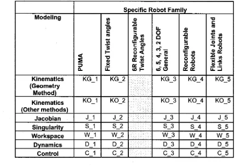
Table 1.1 presents a literature review summary. The highlighted area under the 6R reconfigurable twist angles robot family represents the area that was not covered in literature and was investigated and solved in this research.

T a b le 1.1: L ite r a tu re R e v ie w S u m m a ry M a trix

s

pecific Robot Family

Modeling

P

U

M

A

Fi

xe

d

T

w

is

t

a

n

g

le

s

6R

R

e

c

on

fig

u

ra

bl

e

T

w

is

t

A

ng

le

s

6,

5,

4,

3,

2

D

O

F

G

e

n

e

ra

l

R

e

c

o

n

fig

u

ra

b

le

R

o

b

o

ts

F

le

xi

b

le

Jo

in

ts

a

n

d

Li

nk

s

R

o

b

o

ts

Kinematics

KG 1 KG 2 KG 3 KG 4 KG 5

(Geometry

Method)

Kinematics

KO_1 KO_2 KO_3 KO_4 KO_5

(Other methods)

Jacobian

J_1 J_2 J_3 J_4 J_5

Singularity

S_1 S_2 S_3 S_4 S_5

Workspace

W_1 W_2 W_3 W_4 W_5

Dynamics

D_1 D_2 D_3 D_4 D_5

Control

C_1 C_2 C_3 C_4 C_5

KG_1: (Lee C. S. G „ and Ziegler M „ 1984), (Fu K.S., et al., 1987), (Owens J. P., 1994)

KG_3: (Pashkevich A., 1997)

KG_4: No references found.

KG_5: No references found.

KO_1: (Gu Y. L. and H o J. S., 1990).

KO_2: (Balkan M. T „ e ta l., 2000), (Balkan M. T., e ta l., 2001), (Kohil D „ and A. H. Soni, 1975), (Paul P.R., 1981), (Pennock G. R. and Yang A. T., 1985), (Yang A. T., and R. Freudenstein, 1964), (Uicker J. J. Jr., et al., 1964), (Legnani G., et al., part 1, 1996), (Legnani G., e ta l., part 2, 1996). (Tsai L.W., 1985), (Bekir K. and Serkan A., (2000))

KO_3 : (Tourassis V. D. and Ang M. H. Jr, 1989), (Manseur R. and Doty K. L., 1996), (Manseur R. and Doty K. L., 1992), (Manseur R. and Doty K. L., 1989), (Manseur R. and Doty K. L „ 1988), (Fu H „ et al., 1998). (Fischer I.S., 2000), (Fu

H., e ta l., 2000), (Chapelle F., and Bidaud P., 2001), . (Her M. G., e ta l., 2002)

KO_4: (Matsumaru T., 1995), (Kelmar L. and Khosla P., 1988), (Benhabib B., et al., 1989), (Chen I. M. and Yang G., 1996), (Podhorodeski R. P. and Nokleby S. B., 2000).

KO_5: (Filipovic M., a t a l, 2007).

J_1 : (Orin D. E. and Schrader W. W. 1984), (Fu K.S., et al., 1987), (Corke P. I. 1998).

J_2 : (Orin D. E. and Schrader W. W. 1984), (Leathy M. B., et al., 1987), (Spong M. W. and Vidyasagar M. 1989)

J_4 : No references found.

S_1 : (Cheng F. T., et al., 1997), (Oenny D., et al., 2000), and (Yuan J., 2001), (Fijany A. and Antal K. Bejczy 1988), (Corke P. I. 1998)

S_2 : (Tourassis V. D. and Ang M. H. Jr, 1995), (Gogu G., 2002), (Hayes M. J. D.,

et al., 2002)

S_4 : No references found.

S_5 : No references found.

W_1: No references found.

W_2, W_3: (Shaik M. A. and Datreis P., 1986), (Abdel-Malek K., et al., 2000), (Ceccarelli M., and Vinciguerra A., 1995). (Ceccarelli M., 1996), (Kwan S. J., et al.,

1991), (Hansen J. A., et al., 1983), (Spanos J., and Kohil D., 1985). (Kohil D., and Spanos J., 1985), (Abdel-Malek K „ eta l., 1999), (Zhang H., e ta l., 1991)

W_4: No references found.

W_5: No references found.

D_1: (Yoshida K., et al., 1992), (Izaguirre A., et al., 1992), (Corke P. I., and Armstrong B., 1994), (Corke P. I., 1998), (Walker M. W., and Orin D. E., 1982), (Armstrong B., e ta l., 1986), (Burdick J. W., 1986), (Leathy M. B., e ta l., 1986),

D_2: (Park H. S., and Cho H. C., 1991), (Ju M. S., and Mansour J. M., 1989), (Rajagopalan R.,1996) (Yamakita M., e ta l., 1991), (Featherstone R., and Orin D., 2000), (Palaz H,, e ta l., 1993), (Nathery J. F. and Spong M., 1994)

D_4: No references found.

D_5: (Filipovic M., at al., 2007).

Sandor J. Toth, 1999), (Nagy P. V., 1988), (Dixon W. E., e ta l., 2001), (Moreira N.,

e ta l., 1996), (Goldenberg A. A. and Chan L., 1988).

C_2: This was not investigated.

C_3: No references found.

C_4: No references found.

C_5: No references found.

1.1. Problem Statement

A reconfigurable approach to modeling and designing new manufacturing processes, production, automated machines, software, hardware, and etc., is a current research trend. Automated machines are the essentials of reconfigurable manufacturing. To be able to use them in future reconfigurable manufacturing systems, there is a need to treat them as reconfigurable automated machines. However according to a literature review, the reconfigurable robotic software does not exist yet.

Most of the simulation and off-line programming software is designed so as to provide only robot kinematic models. Usually they have a library of some robots, and if user needs a new robot, they have the option to buy it or to model it with software that they have. This process is sometimes complex and long. The current simulation and off-lining programming software can not be used to perform any reconfigurable control process.

developing reconfigurable parameters. The analysis was done using simulation and off-line programming software Workspace 5®. The eight developed reconfigurable modules (RPF, UKMS, RPGJM, RPFSM, RRW, RPFDM, RPFDM+, and RCP) represent a reconfigurable robot plant model. This solution can be used for any robot that belongs to the RPF group of robots. By simply putting robot information, these eight reconfigurable modules will automatically generate a robot model and its controller.

1.2. Background of Robotics

The development of the industrial robot-arm was of particular importance. Its ability to emulate the serial-link manipulator nature of the human-arm has led to a whole new class of production tasks that may be profitably automated. Examples are paint-spraying, welding, assembly, and pick-and-place operations. More recently, advances in image-recognition, tactile-sensing, and artificial-intelligence have expanded the number of potential applications into those areas where sensory feedback from the environment is required, such as picking up objects which have been randomly placed on a conveyor-belt.

‘Dumb’ manipulators (controlled directly by a human instead of following a computer program) have found further applications in carrying out tasks that might be potentially hazardous to humans. Examples are handling radioactive materials, and manipulating objects underwater or in space (Owens, 1990).

The first robots were introduced in the manufacturing industry in the USA in 1961. Since that time there has been a significant growth in the number of robots in use and the range of applications in which they are used. Today robots play a key role in industrial and manufacturing engineering. In developed countries, many large-scale national and international robot related research and development programs have been launched and are still underway (Ulrich, 1990). There are over 100 robot manufacturers around the world (Djuric A., 1999).

In general, robots may substitute for human operators in the following situations (Groover, 1987):

• Hazardous work environment for human operators

• Repetitive and heavy work cycles

• Parts difficult to handle by human operators

• Infrequent product changeovers

• Part positioning and orientating

Many commercially available industrial robots are widely used in manufacturing and assembly tasks, such as material handling, spot/arc welding, parts assembly, paint spraying, loading, and unloading numerically controlled machines. Some robots are also used in space and undersea exploration, and prosthetic arm research.

1.2.1. Description of a Robot Model

From the study of robotic software Workspace 5® (Workspace 5®, User Manual, 2000) and reviewing literature (Djuric A., 1999), (Armstrong B., et al.,

1986), the following characteristics are commonly used to describe a robot model:

• Robot name

• Number of joints

• Type of joints

• Joint’s positive directions (twist angles a t and joint angles 0t )

• Base frame

• Tool frame

• Link’s lengths d,

• Link’s offsets at

• Link’s mass mi

• Radial distance to the center of mass of each link Pci

• Moment of inertia about a center of mass of each link / ;

The structure of the robot consists of a number of links and joints; a joint will allow relative motion between two links. Two types of joints are used, a revolute joint to produce rotation and a translational joint to produce translation. To achieve

Cartesian

J .

2 Polar Cylindrical

&

2 Jointed Arm SCARA

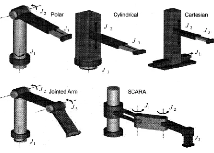
Figure 1.1: Polar, Cylindrical, Cartesian, Jointed Arm, SCARA

For the Polar configuration, the linear extending arm is capable of being rotated around the horizontal and vertical axes. For the Cylindrical configuration, the linear extending arm can be moved vertically up and down in a rotating column. For the Cartesian (Gantry) configuration, there are three orthogonal sliding or prismatic joints. For the Jointed Arm configuration, there are three joints arranged in an anthropomorphic configuration. For the SCARA configuration, there are two rotary axes and a linear joint.

1.2.2. Robot Geometry

description of the spatial displacement of the robot as a function of time, in particular the relations between the joint variable space and the position and orientation of the end-effector of a robot arm.

1.2.2.1 Tool and Base Coordinate frame

Robotic kinematics depends on the use of right handed Cartesian frames of reference. Accordingly, the Tool and Base frames are shown on Figure 1.2.

Tool Frame

Base Frame

Figure 1.2: Tool and Base frames for the PUMA 560 robot

1.2.2.2 Joints

Two types of joints are commonly found in robots: revolute joints, and prismatic joints. Unlike the joints in the human arm, the joints in a robot are normally restricted to one degree of freedom, to simplify the mechanics, kinematics, and control of the manipulator. In general, two links are connected by a lower-pair joint which has two surfaces sliding over one another while remaining in contact. Only six different lower-pair joints are possible: revolute, cylindrical, spherical, planar, prismatic, and screw, Figure 1.3.

Revolute Cylindrical Spherical

Planar _{Prism atic Screw}

Figure 1.3: The lower pair joints

1.2.2.3 Links

A link is a solid mechanical structure, which connects two joints. The main purpose of a link is to maintain a fixed relationship between the joints at its ends. The last link of a manipulator has only one joint, located at the proximal end (the end closest to the base) of the link. At the distal end of this link (the end furthest away from the base) instead of a joint, there is usually a place to attach a gripper: a tool plate. Between the axes of the joints at the ends of any link there can be two degrees of translation and two degrees of rotation. These degrees of freedom are called the link parameters.

1.2.3. Fundamentals of Robot Kinematics

(known as the base frame) will be studied in detail. This transformation specifies the location (position and orientation) of the hand in space with respect to the base of the robot, but it does not tell us which configuration of the arm is required to achieve this location. As we will see, it is often possible to achieve the same end- effector position with many arm configurations.

A serial link manipulator is a series of links, which connects the end-effector to the base, with each link connected to the next by an actuated joint. If a coordinate frame is attached to each link, the relationship between two links can be described with a homogeneous transformation matrix using D-H rules (Denavit J., and Hartenberg R. S, 1955), and they are named '_17j, where i is number of joints. The

first matrix °7j relates the first link to the base frame, and the last 5T6 matrix relates the hand frame to the last link. A sequence of these matrices called the forward kinematic transform of the manipulator is used to describe the transform from the base to the hand of the manipulator.

assigning coordinate frames to links will be developed. To assign a coordinate frame to a link, the relationship between it and the previous link must be understood. This relationship comprises the rotations and translations that occur at the joints.

1.2.3.1 Denavit - Hartenberg Notation

Each joint is assigned a coordinate frame. Using the Denavit-Hartenberg notation (Denavit J., and Hartenberg R. S, 1955), 4 parameters are needed to describe how a frame / relates to a previous frame i - 1 .

As seen in Figure 1.4, the zr axis points along the i th axis. The origin of the

i th frame is on the i th axis at the point of the common perpendicular with the i +1 frame. The xr axis points along the perpendicular, or if the axes intersect, xt is normal to the plane containing the two axes. The y r axis completes a right- handed coordinate system.

After assigning coordinate frames the four D-H parameters can be defined as following (Figure 1.4):

at - Link length is the distance along the common normal between the joint axes

a,-Tw ist angle is the angle between the joint axes

Joint angle is the angle between the links

dr Link offset is the displacement, along the joint axes between the links

Joint n+]

Link n- 1

Figure 1.4: Coordinate frames and D-H parameters

Between two frames we have a kinematic relationship, two translations and two rotations:

• Translate along a length aM

• Rotate about the twist angle a M

• Rotate about dt an angle 6t

• Translate along zt a distance dt

This relationship is mathematically represented by a 4 x 4 Homogeneous Transformation Matrix in Equation 1.

Kfe

Y M , ) =

cos di - cos a t sin 6i

sin 6t cos a i cos 0i

0 0

sin (Xi

sin a i sin di at cos 6t - sin a i cos 6t at sin a t

di

0 1

The robot can now be kinematically modeled by using the link transforms:

0Tn=°Tl lT22Tr --i-l Tr --n~l Tn (2)

Where °Tn is the pose of the end-effector relative to base; is the link

transform for the i th joint; and n is the number of links.

1.3. Research Approach

To compare and contrast the different solutions for robot modeling, robot kinematics, dynamics and control, first a literature review was performed, which is covered in Chapter 1.

The reconfigurable robot modeling approach and reconfigurable inverse kinematic solution is presented in detail in Chapter 2. The examples of the ABB IRB1400 and the Fanuc ARCMate120iL robots are used to show the capability of UKMS and to verify inverse kinematic results.

In a Chapter 3, two reconfigurable modules are developed. The first one is the RPFJM. All elements of this matrix are presented in Appendix A. The examples of PUMA group Jacobian named RPJM and the example of the Fanuc group Jacobian named RFJM are presented in Appendix B and Appendix C respectively, second reconfigurable module is the RPFSM. The complete result is in Appendix D. The example for the PUMA and Fanuc cases are the RPSM and the RFSM and their results are in Appendix E and Appendix F respectively. The complete reconfigurable calculation program for RPFJM written in MAPLE 10® is presented in a Technical Document (Djuric 2007).

The reconfigurable PUMA-Fanuc dynamic model (RPFDM) is developed in Chapter 5. The reduced reconfigurable PUMA 560 dynamic parameters as a function of th e i£ 6 parameter are given in Appendix G. The complete reconfigurable calculation program for RPFDM model written in MAPLE 10® is presented in a Technical Document (Djuric 2007). The extended RPFDM+ model includes DC motors for each link. All motor information is shown in Chapter 6.

The design of the Reconfigurable Control Platform (RCP) for the PUMA 560 is done in Chapter 6. The sizing of the DC motors is done in detail. The reconfigurable “PI” controller for joint position control is designed as a function of robot motor parameters. Simulation is done using Matlab/Simulink ® software. The future work and conclusions are presented in Chapters 7 and 8 respectively.

CHAPTER TWO

2. GENERALIZED RECONFIGURABLE 6 - JOINT ROBOT

MODELING

2.1. Introduction to Unified Reconfigurable Open Control

Architecture (UROCA)

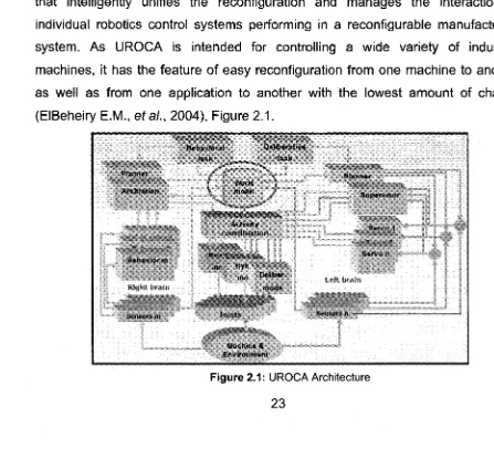
This research is a part of the UROCA (Unified Reconfigurable Open Control Architecture) project, which aims to develop a highly reconfigurable control system that intelligently unifies the reconfiguration and manages the interaction of individual robotics control systems performing in a reconfigurable manufacturing system. As UROCA is intended for controlling a wide variety of industrial machines, it has the feature of easy reconfiguration from one machine to another as well as from one application to another with the lowest amount of change (ElBeheiry E.M., eta l., 2004), Figure 2.1.

ii§>

A ifivity

j l I

Deiiber

mod*

Joints

The goal of this research is to develop reconfigurable World Models for robotic applications, and its position in UROCA is circled in Figure 2.1.

The graphical representation of the UROCA architecture in Figure 2.1 is inspired by human learning principles and the right brain, left brain and whole brain design methodologies. For robotic applications, the left planner, using a world model, performs tasks related to command decoupling, path generation, trajectory planning, kinematics inversion, dynamics calculation, etc. To be able to perform any reconfigurable control process, a reconfigurable plant model that represents different robotic systems, needs to be develop.

2.2. Reconfigurable Aspects of Industrial Robotic Systems

There is a strong possibility here for the UROCA architecture to switch from one template to another, rather than switch from one individual robot model to another.

Most of the current research has been done in the area of modeling modular and reconfigurable robots, machines, reconfigurable controls and software for the modular systems. There is no reconfigurable software or controller designed for existing industrial robots.

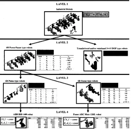
To be able to design a reconfigurable controller for existing robots, no one must know what is reconfigurable; the robot’s reconfigurable aspects must be found. From the analysis of many industrial robots came with the classification presented in Figure 2.2. This classification has four reconfiguration levels and each level has its own groups of robots:

Level 1

: All Industrial robots belong to one group.

Level 3: The first group is 6R PUMA type robots, and the second group is 6R Fanuc type robots.

Level 4: Specific single robots from each of the two groups in Level 3 represent their own groups.

LAVELl

Industrial Robots

LAVEL2

6R Puma-Fanuc type robots _{Translational and/or rotational 3-4-5 DOF type robots}

&

180:0

4

X

± 1 8 0 :0

LAVEL 3

6R Puma type robots 6R Fauuc type robots

Joint 0, d

0 -90

0 0 90

6 A r fj ^ ±18 0 ; 0 -90

90 ± 1 8 0 :0

LAVEL 4

ABB IR B 1400 robot Fanuc ARC Mate 120IL robot

C ^ iY = co nst 0i9d i9l t = co nst

Join!.. Thatal

1 -36000 475.00

2 -30.00 aoo

3 180.00 aoo

4 aoo 720.00

5 aoo aoo

6 0 0 0 85.05

Al Atohel

150.00 600.00 -120.00 aoo aoo aoo -saoo aoo 90.00 -90.00 9a oo aoo

( K j Y = c o n s t 0 , , d , , l, = co n s t

Theta

0.00 700.05 20000 -90.00 0.00 800.00 180.00 0.00 -mOO aoo -813.00 aoo

0.00 0.00 0.00

aoo -100.00 aoo -90.00 180.00 90.00 •90 00 90.00 0.00

Figure 2.2: Classification of Industrial robots

need to develop a reconfigurable kinematic module using all the information from the analysis of the robots’ similarities and differences, and the robots’ reconfigurable parameters. From Figure 2.2 can be recognized a group o f 6R PUMA-type and Fanuc-type robots which represent RPF model.

2.3. Development of the RPF Model

As a preliminary step towards having the RPF model, kinematic structures of 197 different industrial robots from 11 different manufacturers where analyzed: ABB, Adept, Comau, Fanuc, Kawasaki, Kuka, Motoman, Nachi, Panasonic, Staubli, and Daihen. The results are reported in Table 2.1. Listed robots in bold are PUMA type, underlined are Fanuc type and italic are others.

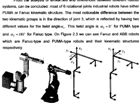
From the analysis of similarities and differences between different robotic systems, can be concluded: most o f 6 rotational joints industrial robots have either PUMA or Fanuc kinematic structure. The most noticeable difference between the two kinematic groups is in the direction o f joint 3, which is reflected by having two different values for the twist anglea 2. This twist angle is a 2 =0° for PUMA type

and a 2 =180° for Fanuc type. On Figure 2.3 we can see Fanuc and ABB robots which are Fanuc-type and PUMA-type robots and their kinematic structures respectively.

Figure 2.3: Fanuc-type and PUMA -type robots and their joint three directions