Optical Properties of Nanostructures and Applications to Surface-Enhanced Spectroscopy

University of Windsor University of Windsor

Scholarship at UWindsor

Scholarship at UWindsor

Electronic Theses and Dissertations Theses, Dissertations, and Major Papers

2009

Optical Properties of Nanostructures and Applications to

Optical Properties of Nanostructures and Applications to

Surface-Enhanced Spectroscopy

Enhanced Spectroscopy

Daniel Ross

University of Windsor

Follow this and additional works at: https://scholar.uwindsor.ca/etd

Recommended Citation Recommended Citation

Ross, Daniel, "Optical Properties of Nanostructures and Applications to Surface-Enhanced Spectroscopy" (2009). Electronic Theses and Dissertations. 473.

https://scholar.uwindsor.ca/etd/473

This online database contains the full-text of PhD dissertations and Masters’ theses of University of Windsor students from 1954 forward. These documents are made available for personal study and research purposes only, in accordance with the Canadian Copyright Act and the Creative Commons license—CC BY-NC-ND (Attribution, Non-Commercial, No Derivative Works). Under this license, works must always be attributed to the copyright holder (original author), cannot be used for any commercial purposes, and may not be altered. Any other use would require the permission of the copyright holder. Students may inquire about withdrawing their dissertation and/or thesis from this database. For additional inquiries, please contact the repository administrator via email

OPTICAL PROPERTIES OF NANOSTRUCTURES AND APPLICATIONS TO

SURFACE-ENHANCED SPECTROSCOPY

BY

DANIEL JOSEPH ROSS

A Dissertation

Submitted to the Faculty of Graduate Studies through the

Department of Physics in Partial Fulfillment of the

Requirements for the Degree of Doctor of Philosophy at

The University of Windsor

Windsor, Ontario, Canada

2009

Optical Properties of Nanostructures and Applications to Surface Enhanced

Spectroscopy.

By

Daniel Joseph Ross

APPROVED BY

_________________________________________ Dr. Cecilia Noguez, External Examiner

Instituto de Fısica, UniVersidad Nacional Autonoma de Mexico,

_________________________________________ Dr. S. Holger Eichorn

Department of Chemistry and Biochemistry

_________________________________________ Dr. Chitra Rangan

Department of Physics

_________________________________________ Dr. Roman Maev

Department of Physics

_________________________________________ Dr. Ricardo Aroca, Advisor

Department of Chemistry and Biochemistry

_________________________________________ Dr. Jichang Wang

DECLARATION OF CO-AUTHORSHIP

I hereby declare that this dissertation incorporates material that is result of joint research, as follows:

This dissertation incorporates the outcome of joint research undertaken with Mathew Halls, under the supervision of Ricardo Aroca and Gholam Abbas Nazri of GM Research laboratories. The results of this collaboration are detailed in Chapter 8, section B of this dissertation. In this case the primary contributions, data analysis, and interpretation were all performed by the author. Contribution of Mathew Halls was primarily through advice on use of high level computational tools in cluster based research, while Gholam Abbas Nazri provided the

materials, as well as details and expertise on synthesis.

This dissertation also includes the outcome of joint research undertaken with Dr. R. E. Clavijo of the University of Chile. The results of this collaboration are detailed in chapter 8, section C. In this case, the experimental Raman, SERS, and infrared spectra were obtained by Dr. Clavijo, who granted permission for their use.

I am aware of the University of Windsor Senate Policy on Authorship and I certify that I have properly acknowledged the contribution of other researchers to my thesis, and have obtained written permission from each of the co-author(s) to include the above material(s) in my thesis.

I certify that, with the above qualification, this thesis, and the research to which it refers, is the product of my own work.

DECLARATION OF PREVIOUS PUBLICATION

This thesis includes 2 original papers that have been previously

published/submitted for publication in peer reviewed journals, as follows:

Thesis Chapter

Publication title/full citation Publication

status Chapter 8,

section C

Surface Enhanced Raman Scattering of trans-p-Coumaric and Syringic Acids

Accepted

Chapter 8, Section B

Raman scattering of complex sodium aluminum hydride for hydrogen storage/Daniel J Ross, Mathew D Halls, Abbas G Nazri and Ricardo F Aroca,

Chemical Physics Letters, 388, 430, 2004

Published

Chapter 7 Surface enhanced infrared spectroscopy /R.F. Aroca,

D. Ross, and C. Domingo, Applied Spectroscopy, 58, 324-338A., 2004.

I certify that I have obtained a written permission from the copyright

owner(s) to include the above published material(s) in my thesis. I certify that the above material describes work completed during my registration as graduate student at the University of Windsor.

I declare that, to the best of my knowledge, my thesis does not infringe upon anyone’s copyright nor violate any proprietary rights and that any ideas, techniques, quotations, or any other material from the work of other people included in my thesis, published or otherwise, are fully acknowledged in

accordance with the standard referencing practices. Furthermore, to the extent that I have included copyrighted material that surpasses the bounds of fair dealing within the meaning of the Canada Copyright Act, I certify that I have obtained a written permission from the copyright owner(s) to include such material(s) in my thesis.

ABSTRACT

Metallic nanoparticles, in particular silver and gold nanostructures, are at

the centre of the development of plasmon enhanced optical signals. There is a

flurry of activities in the fabrication and testing of these nanostructures, especially

in surface enhanced Raman scattering (SERS) and surface enhanced-infrared

absorption (SEIRA), the two branches of surface-enhanced vibrational

spectroscopy. The need to develop an understanding of this general subject

matter for practicing spectroscopists cannot be questioned. This work is a unique

undertaking intended to examine some of the elements that give rise to

surface-enhanced spectroscopy.

The optical properties of nanoparticles are discussed in detail, beginning

with a discussion of the electromagnetic theory describing the interaction of light

and matter. Exact solutions to the electromagnetic equations are used to model

and calculate plasmonics of nanoparticles. These methods include Mie theory,

and extensions to Mie such as for concentric spheres and interacting spheres.

Approximate methods are also discussed, such as the dipolar model for

ellipsoids of rotation, and the coupled dipole equations for irregular or interacting

particles. These models are used to obtain optical properties as well as

enhanced electromagnetic fields, applied to surface enhanced vibrational

spectroscopy. The origin of vibrational spectroscopy is briefly described, and

quantum mechanical calculations are performed to describe a variety of the

molecular possibilities arising through surface enhanced spectroscopy, such as

DEDICATION

ACKNOWLEDGEMENTS

An enormous number of people have been a part of my work during my

PhD, and it is a monumental, albeit extremely enjoyable, task to enumerate and

thank each one.

First, my family, especially my parents, Fred and Catherine, have never

questioned my ability to do this. My siblings and their spouses, Neil, Tara,

Gerard, Jenny, and Caroline, have always been extremely supportive. My other

family, including Laurel, James, John, and Dorothy-Anne have also been a

source of encouragement and strength. Catherine and Laurel, especially, are

thanked for their prowess at editing. All remaining errors are mine alone. It goes

without saying that Hank has probably been my most loyal fan throughout the

process.

The Department of Physics has been gracious to provide me with support,

both financial and in terms of available resources, and most of all, a knowledge

base on which to stand. The staff in the Department of Chemistry have also

been part of my support network many times.

Working on a dynamic and vibrant research team like the Materials and

Surface Science group has been an experience that will stay with me forever. I

would like to thank all present and past members for their contributions to my

learning. Special acknowledgements go to Nik Pieczonka, Paul Goulet,

Teodosio del Caño, Ramon Alvarez-Puebla, Carlos José Constantino, and

Abbas Nazri for invaluable discussions and generosity with their expertise. Extra

special thanks to Mathew Halls, who shared many hours of his time to give me

an insight into quantum chemistry enjoyed by very few. Ricardo Aroca has been

a supervisor about which I have boasted on many occasions, providing

knowledge, support, resources, a lifetime of experience, and friendship.

Although “I couldn’t do it without you” is a cliché, it has rarely been more true.

Lastly, the acknowledgement my wife Reagan Gale Ross deserves would

require a dissertation longer than this one. Her patience, encouragement, and

TABLE OF CONTENTS

DECLARATION OF CO-AUTHORSHIP/PREVIOUS PUBLICATION iii

ABSTRACT v

DEDICATION vi

ACKNOWLEDGEMENTS vii

LIST OF TABLES x

LIST OF FIGURES xi

LIST OF APPENDICIES xvii

LIST OF SYMBOLS, ABBREVIATIONS, AND NOMENCLATURE xviii

CHAPTER

I. INTRODUCTION 1

A. Plasmonics and Optical Properties of Nanoparticles 1

B. Definition of The Optical Constants 5

C. Surface Enhanced Spectroscopy 13

D. Bibliography 17

II. MIE THEORY 19

A. Solution for Maxwell’s Equations for a Sphere 19

B. Expansion of Incident Field 28

C. Scattered and Internal Fields 33

D. Extinction and Scattering Cross Sections 36

E. Calculation of the Near Field 50

F. Bibliography 58

III. NANOSHELLS 59

A. Theoretical Background 59

B. Results 64

C. Bibliography 72

IV. DIPOLE APPROXIMATIONS AND THE COUPLED DIPOLE EQUATIONS

74

A. Non-Spherical Shapes Through the Dipolar Approximation

74

B. Non-Spherical Shapes Through the Coupled Dipole Equations

81

D. Bibliography 97

V. EXTENDED MIE THEORY 98

A. Theory of Cooperative Scattering 98

B. Addition Coefficients for Vector Spherical Harmonics 106

C. Calculation of the Near Field 108

D. Normal Incidence 115

E. Particles along a Common Z-axis 119

F. Field at a Point on the Z-axis 121

G. Asymptotic Expansion for Large Separation 125

H. Rayleigh Regime for Identical Particles 132

I. Extinction Cross Sections and Field Calculations 145

J. Bibliography 151

VI. QUANTUM OPTICAL MODEL OF SURFACE ENHANCED SPECTROSCOPY

152

A. Unified Surface Enhanced Spectroscopy Through Quantum Optics

152

B. Quantum Optical Results from Couple Particles 161

C. Bibliography 163

VII. SURFACE ENHANCED INFRARED ABSORPTION (SEIRA) 164

A. Introduction to Surface Enhanced Infrared Absorption 164

B. Effective Medium Theories 170

C. A Model SEIRA Case 175

D. Bibliograpy 181

VIII. QUANTUM CHEMISTRY FOR MOLECULAR SYSTEMS 184

A. Nanostructures and the Observed Spectra in SER(R)S 184

B. Materials for Hydrogen Storage 192

C. SERS Study Case 203

D. PTCDA 215

E. Bibliography 218

IX. CONCLUSION 220

A. Biblography 223

APPENDICIES

A. Couple Dipole Equation Program for C++ 224

B. Mie Scattering, Extinction, and Near Field Calculations 230

C. Copyright Releases 233

VITA AUCTORIS 238

LIST OF TABLES

Table 2.1. Computed extinction results for silver spheres. 40

Table 2.2. Computed scattering results for silver spheres. 42

Table 2.3. Comparison of extinction, scattering, and absorption cross sections and efficiencies for silver spheres

44

Table 2.4. Scattered field peak wavelength, relative intensity, FWHM, and scattering efficiency for silver spheres varying radii.

52

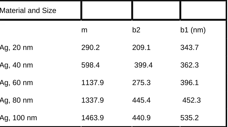
Table 3.1. Calculated parameters for use in equation 3.7, from Mie calculations

67

Table 6.1: Differential cross section results. Intensities are in units of 10

-18

cm2/(meV sr).

162

Table 8.1. Geometric parameters and relative energies for monomers of

NaAlH4, in bidentate, tridentate, and monodentate configurations. (Lower

numbered hydrogen are those bonded to Na in all three cases)

197

Table 8.2:. Wavenumbers and vibrational assignments of observed

Raman bands of NaAlH4.

200

Table 8.3: Character table of syringic and p-coumaric acid. Acronyms include ip: in-plane, and oop: out of plane.

206

Table 8.4: Observed and calculated Raman wavenumbers (cm-1) of

syringic acid and its Ag-complex and SERS on Ag colloids

211

Table 8.5: Observed and calculated infrared spectra of syringic acid. 212

Table 8.6: Calculated Infrared frequencies and intensities for PTCDA at B3LYP/6-31g(d) level of theory. oop and ip are acronyms designating “out of plane” and “in plane”, respectively.

LIST OF FIGURES

Figure 1.1 Illustration of surface charge and electric field in a surface plasmon.

2

Figure 1.2. Schematic of Raman scattering (RS), resonant Raman scattering (RRS), Infrared Absorption (IR), and Fluorescence.

15

Figure 2.1. Extinction, absorption, and scattering cross sections for a 30nm silver sphere.

38

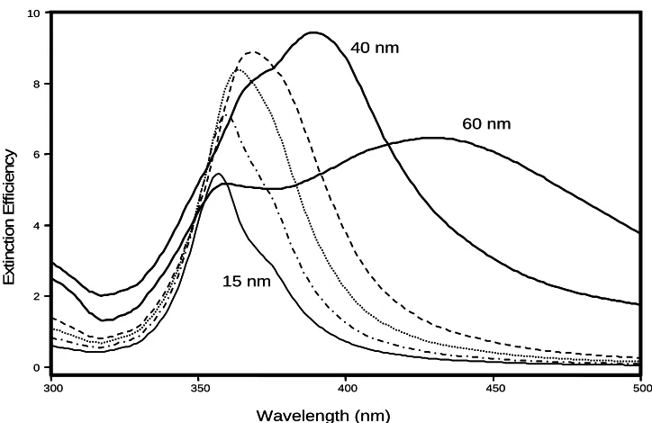
Figure 2.2. Extinction efficiency of silver spheres of varying radii. 39

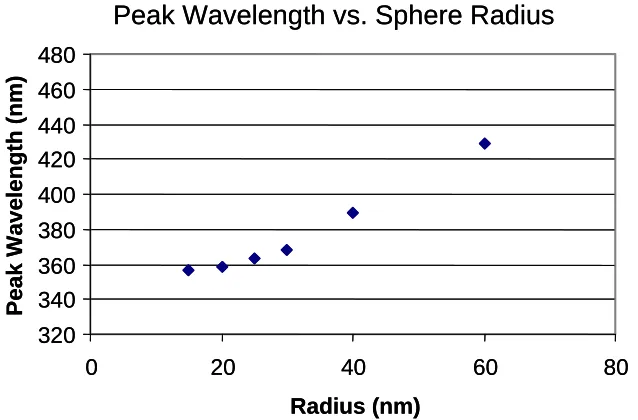
Figure 2.3. Peak wavelength of main peak vs. radius for silver spheres. 41

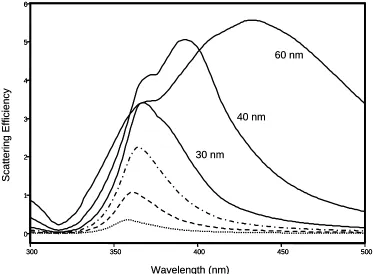
Figure 2.4. Scattering efficiency of silver spheres of varying radii. 42

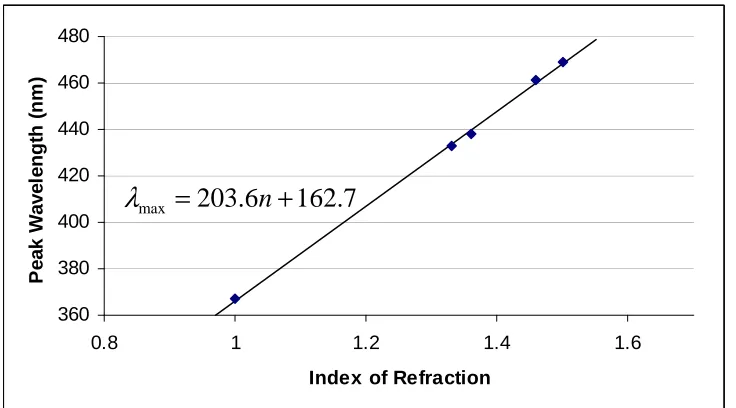
Figure 2.5. Scattering cross sections of 30 nm silver particles in a variety of media.

45

Figure 2.6. Plot of peak wavelength vs. Index of Refraction. 45

Figure 2.7 Real part of dielectric functions of Silver (solid), Gold (dotted) and Copper (dashed)

46

Figure 2.8. Real part of dielectric functions of Silver (solid), Gold (dotted) and Copper (dashed)

46

Figure 2.9: Extinction cross sections of Copper, Gold, and Silver. 47

Figure 2.10: Scattering cross sections of Gold, Copper (dashed) and Silver.

48

Figure 2.11: Scattered field by silver spheres of varying radii. 51

Figure 2.12 Plot of relative scattered field intensities (triangles) and extinction efficiencies divided by the cube of the radius (squares), as a function of radius.

52

Figure 2.13. Plot of relative scattered field intensity against volume normalized scattering efficiency.

53

Figure 2.14. Relative scattered field intensity of silver, gold (dotted), and copper as a function of wavelength

Figure 2.15. Scattered Field Intensities for 20 and 30 nm Silver Particles. 55

Figure 2.16 Relative scattered field intensity as a function of distance from surface for 20nm (solid), 25 nm (dotted), and 30 nm (dashed) silver spheres.

56

Figure 2.17 Natural logarithm of relative scattered field intensity as a function of distance from surface for 20nm (solid), 25 nm (dotted), and 30 nm (dashed) silver spheres.

57

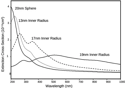
Figure 3.1. 20 nm outer radius of Ag: a) Solid line, sphere. b) Long dash, 11 nm inner radius. c) Short dash, 17 nm inner radius. d) dotted line, 19 nm inner radius.

65

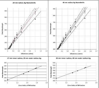
Figure 3.2: Peak wavelength vs. inverse shell thickness for Ag nanoshells of 60 nm outer radius, and peak wavelength vs. core index of refraction for 0.587 core/shell volume ratio for Ag nanoshells of 60nm outer radius.

65

Figure 3.3: Peak wavelength vs. inverse shell thickness for Ag nanoshells of 20 and 40 nm outer radius, and peak wavelength vs. core index of refraction for 0.587 core/shell volume ratio for Ag nanoshells of 20 and 40nm outer radius.

66

Figure 3.4. Extinction Cross Section of Ir nanoshells, outer radius 20nm, vacuum core

68

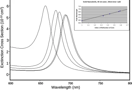
Figure 3.5. Plasmon response of Au nanoshells, 40 nm outer radius, 34 nm inner radius, for vacuum, aqueous, silica, dendrimer, and polystyrene cores.

69

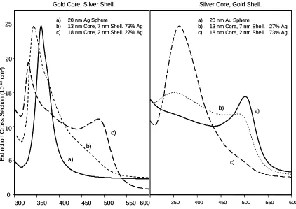
Figure 3.6. Plasmon response of silver/gold and gold/silver core/shell systems.

70

Figure 3.7. Plasmon response of silver/gold and gold/silver core/shell systems, contrasted with mixtures from effective medium theory, for 27% Ag by volume.

71

Figure 4.1: Extinction cross section of a gold nanorod of aspect ratio 4 considering only the minor axis.

77

Figure 4.2 Extinction cross section of a gold nanorod of aspect ratio 4 considering only the major axis.

77

Figure 4.4. Extinction cross section of a gold nanorod of aspect ratio 4 in different media: Vacuum(εm=1), Water(εm=1) (dotted), Benzene(εm=1.5)

(dashed), and εm=1.75 (dot-dash).

79

Figure 4.5: Extinction cross sections for gold spheres and nanorods, with major axis 25 nm, corresponding to sphere, aspect ratio of 2 (dotted), aspect ratio of 3 (dashed), aspect ratio of 4 and aspect ratio of 6.

80

Figure 4.6: Spheres made up of 136 dipoles (left) and 304 dipoles (right). 83

Figure 4.7: Extinction cross sections of 10 nm sphere using Mie (solid), CDE using 136 dipoles (dashed), CDE using 304 dipoles (dotted).

83

Figure 4.8 Extinction cross sections of 50 nm sphere using Mie (solid), CDE using 136 dipoles (dotted), CDE using 304 dipoles (dashed), CDE using 1024 dipoles (dot-dashed)

84

Figure 4.9: Discretization of a 380 dipole cylinder of aspect ratio 4. 85

Figure 4.10: Extinction of a gold cylinder of major axis 25 nm, and minor axes 6.25 nm.

85

Figure 4.11 Schematic of particle arrangement for calculation of

enhancement. The particles of radius R are separated by a distance d.

88

Figure 4.12: Field enhancement as a function of wavelength for 2 particle system.

89

Figure 4.13 : Arrangements of particles. 1 and 2 represent the positions of a single particle and dimer respectively, while 3a and 3b refer to the two different configurations of a 3 particle system.

90

Figure 4.14: Extinction cross section vs. Incident Wavelength for 1 (solid), 2 (dashed), and 3 particles, in configuration 3a (dot-dash) and 3b (dotted).

91

Figure 4.15. Electric field enhancement vs. Wavelength for 1 particle sampled at S1 (solid), 2 particles sampled at S1 (dashed), and 3 particles

(dotted line), in configuration 3a sampled at S1, and 3b sampled at S2 and

S4. The inset shows detail of the single particle and configuration 3a

from 300 to 450nm.

92

Figure 4.16: Electric field enhancement for 1 particle at 356 nm (left) and 2 particles at 428 nm (right).

Figure 4.17: Electric field enhancement for 3 particles in configuration 3a at 426 nm (left) and 342 nm (right).

94

Figure 4.18: Electric field enhancement for 3 particles in configuration 3b

at 530 nm. 94

Figure 4.19: Self-avoiding random walks of 100 particles. 95

Figure 4.20: Extinction cross section of 20 nm silver particles for the configurations seen in Figure 4.19.

96

Figure 5.1: Ray diagram of the scattering events considered in order of scattering method.

111

Figure 5.2. Schematic of two particles along z axis. 132

Figure 5.3: Extinction cross section of two interacting 30 nm silver spheres, with surface separation of infinity (solid), 2 nm (dotted), 1 nm (dashed), and in contact (dot-dash)

145

Figure 5.4: Extinction cross section of two 20nm particles at a distance of infinity (dotted), 8 nm, 4 nm (dashed), 2 nm (dot-dash), and in contact.

146

Figure 5.5: Field enhancements for 20nm particles with surface separations of 4 nm, 2 nm, and in contact.

147

Figure 5.6: Enhancement for two 20 nm silver particles. In contact, field enhancement (solid) and damping enhancement (dotted), at 2 nm

surface separation, field enhancement (dashed) and damping enhancement (dot-dash)

148

Figure 5.7: Electric field enhancement for 2 20nm silver particles. 148

Figure 5.8: Electric field enhancement for 3 20nm silver particles in a triangular formation.

149

Figure 5.9: Electric field enhancement for 3 20nm silver particles in a straight line.

149

Figure 6.1. Scattering and Fluorescence cross sections for d=0, 1, 2, and

4 nm. The parameters used are: ħωL=2.45 eV, : ħωge=2.35 eV,

ħωvib=0.16 eV, γph=1x1014 Hz, α=0.5, and E0=1x104 N/C.

161

Figure 7.1: Enhancement factor of the electromagnetic field for spheroids in vacuum, with lengths of 90 and 30 nm for major and minor axes

respectively

Figure 7.2: Real and Imaginary parts of the dielectric function for Silver and Tin.

168

Figure 7.3: Enhancement factor for SiC averaged over the surface of a particle with the same computational parameters as those in Figure 7.1

169

Figure 7. 4: Maxwell-Garnet computation for a collection of prolate ellipsoids, with a major axis of 90 nm and a minor axis of 30 nm, coated with a 1 nm thick layer of PTCDA.

174

Figure 7.5: Planar, D2h PTCDA molecule. 175

Figure 7.6: DFT B3LYP/6-31g(d) computation results, and the transmission FTIR spectrum of PTCDA in a KBr pellet.

177

Figure 7.7: RAIRS spectrum of a 50 nm PTCDA film deposited onto smooth reflecting silver mirror and calculated vibrational intensities for the b3u species.

177

Figure 7.8. Transmission spectra. PTCDA pellet, SEIRA spectrum, and 50 nm film on KBr crystal.

178

Figure 7.9. SEIRA spectrum of the 10 nm PTCDA film on 15 nm silver island film. RAIRS spectrum of the 10 nm PTCDA film on smooth silver mirror, and transmission FTIR spectrum of the 10 nm PTCDA film on KBr crystal.

179

Figure 8.1. Eight monomer cluster of NaAlH4 optimzed at the

B3-LYP/6-31+G(d,p) level of theory.

195

Figure 8.2. Raman scattering of NaAlH4 using the 633 nm excitation line. 196

Figure 8.3. Simulated and experimental Raman spectra for the high

frequency region of NaAlH4 using the largest cluster model and the

633nm laser line, top and bottom trace respectively. Inset: Calculated high-frequency Raman for the one, two, four, six, and eight monomer models.

198

Figure 8.4. Simulated and experimental Raman spectra for the middle

frequency region of NaAlH4 using the largest cluster model and the

633nm laser line, top and bottom trace respectively. Inset: Calculated mid-frequency Raman for the one, two, four, six, and eight monomer models.

Figure 8.5. Simulated and experimental Raman spectra for the low

frequency region of NaAlH4 using the largest cluster model and the

633nm laser line, top and bottom trace respectively. Inset: Calculated low-frequency Raman for the one, two, four, six, and eight monomer models.

199

Figure 8.6: Syringic acid (left) and p-coumaric acid (right). 203

Figure 8.7: Calculated Raman spectra of: P-coumaric acid (top) and syringic acid (bottom).

204

Figure 8.8: Structure of syringic acid (left) and p-coumaric (right). 207

Figure 8.9: Raman spectra of syringic acid (bottom) and syringic silver salt (top). The spectrum of the syringic salt is offset for clarity.

208

Figure 8.10: Raman spectra of p-coumaric acid (bottom) and p-coumaric silver salt (top). The spectrum of the syringic salt is offset for clarity.

209

Figure 8.11: Difference spectra of p-coumaric (top) and syringic (bottom).

210

Figure 8.12. Raman and SERS spectra of syringic acid. 213

Figure 8.13: Raman intensity of yy elements of polarizability tensor of p-syringic acid.

214

Figure 8.14: Raman and SERS spectra of coumaric acid. 214

Figure 8.15. Computed infrared spectrum of PTCDA at B3LYP/6-31g(d), with classification of bands according to character.

LIST OF APPENDICIES

224 230 A. Couple Dipole Equation Program for C++

B. Mie Scattering, Extinction, and Near Field Calculations

LIST OF SYMBOLS, ABBREVIATIONS, AND NOMENCLATURE

AFM: Atomic Force Microscopy

LSPR: Localized Surface Plasmon Resonance

RRS: Resonance Raman Scattering

RS: Raman Scattering

SAW: Self Avoiding Walk

SEF: Surface Enhanced Fluoresence

SEIRA: Surface Enhanced Infrared Absorption

SERRS: Surface Enhanced Resonance Raman Scattering

SERS: Surface Enhanced Raman Scattering

CHAPTER ONE INTRODUCTION

A. Plasmonics and Optical Properties of Nanoparticles

The following dissertation may best be understood to be part of the field of

plasmonics. Plasmonics is the study of the electronic oscillation, or plasmon,

which is created by the interaction of light with a nanostructured material.1 It is the optical response of noble metals, dominated by the behavior of their

conduction electrons, which can produce collective oscillations of the electrons,

or, plasmon. The interaction between electromagnetic radiation (from infrared to

the ultraviolet) and a metal surface may lead to surface plasmon excitation, as

this interaction creates electronic plasma oscillations on the surface of the metal.

When speaking of a plasmon, it is necessary to differentiate whether the

collective excitation of electrons of the metal is contained within the metal or is a

surface excitation.

Should the excitation be found within the metal (e.g., bulk plasmons), the

oscillations due to fluctuations in the electronic density of the metal are

longitudinal2-4. In this case, the condition for plasmon formation is that the real part of the dielectric function is zero, which is only true at a specific frequency of

light. This frequency is termed the plasma frequency, and, in practice, is very

distinctive among different materials. For metallic surfaces, however, there

exists a surface plasmon with an amplitude that dies off quickly away from the

surface. This surface excitation is a coupling of the incident photons with the

oscillation of the conduction electrons and it polarizes the surface. The surface

plasmon is often thus referred to as the surface plasmon-polariton, clearly

indicating that this excitation is a coupling of the light and a material. This

concept is shown in Figure 1.1, which is an idealized image of the charge, and

Figure 1.1 Illustration of surface charge and electric field in a surface plasmon.

The electromagnetic field of a surface plasmon at the metal/dielectric

interface is the evanescent solution of Maxwell’s equations, applying the correct

continuity conditions at the surface. This work deals with the surface plasmons

in a specific size regime: that of metal nanoparticles. These excitations depend

strongly on both the size and shape of the particle or particles involved, and thus

are very different from the surface plasmon created in a flat surface. These are

often termed localized surface plasmons, or localized surface plasmon

resonances (LSPR), as they are confined to nanometric particles, leading to

resonances that depend on the size, shape, and dielectric function of the material

that the particle is made up of. Discussing the solution of Maxwell’s equations for

this problemwill be one of the main subjects of this work.

Although plasmonics is a relatively new field, (the term was first appeared

in the literature in 2001)5 , the study of plasmons has had a much longer history.

For example, the use of colloidal gold and silver particles in the Lycurgus cup

give it unique optical properties6. These gold and silver particles, as will be shown in detail later (See chapter 2, p.18) absorb and scatter light primarily in the

shorter wavelengths of the visible region. When viewed using reflected light, the

cup is a green colour. When lit from inside, however, the gold and silver particles

historic application for the scattering of light by metal particles is seen in the

windows of temples, churches, and other buildings, as well as in other forms of

stained glass artwork. The bright colours of the stained glass are due to metallic

nanoparticles, the specific colour depending on the size and material of the

particle.

The first systematic understanding of the phenomenon that would later

develop into the field of plasmonics was through Mie’s solution to Maxwell’s

equations for a dielectric sphere8. The exact solution of the interaction of light with a spherical body was now understood, given that the optical properties of

the specific material were known. In addition to colloidal metal particles, Mie’s

solution applies to a wide variety of problems 9: atomospheric dust, interstellar

particles, solar coronas, scattering by raindrops10, and others. The theory of

electromagnetic absorption and scattering by small particles, as well as

applications and computational techniques has been summarized by Kerker11

and Bohren and Huffman10.

Given the wide variety of techniques to fabricate nanoparticles, there are a

plethora of possible shapes and sizes, even for the two most common materials,

silver and gold. Although spheres are probably the most common (due to the

relative ease of synthesis through colloidal suspensions of gold and silver) some

of the geometrically simple, yet interesting shapes include nanoshells12-15,

ellipsoids of revolution16, triangles17, cubes18, and hexagons19. These latter shapes make up a fairly small sample that reveals possibility of modifying the

nanoparticle shape. Fortunately, this modification of shape allows for control

over the resonance wavelength, amplitude, and bandwidth. Another important

development is that of interacting particles, such as dimers of spheres and

shells20, and of triangles17, forming nano ‘bow-ties’. The problem of two interacting particles is one of the few that can be treated exactly, or at least

approximated well, while still having some of the essential features of a system of

particles.

The confinement of electromagnetic field to the particle gives the surface

used for studying adsorption on the surface, as well as surface roughness and

related phenomena. Devices based on the surface plasmon are used in chemical

and biological sensors21. The enhancement of the electromagnetic field at the

interface is responsible for phenomena such as optical amplification surface: the

intensification of the surfaces by Raman scattering (SERS), where it is possible

to detect a single molecule; second harmonic generation; fluorescence, and so

on. In addition, the two-dimensional nature of the surface plasmon makes it

particularly interesting in building plasmon circuits, where the information is

transmitted through a surface plasmon, with potential applications in optical

computing. The fabrication, manipulation, and characterization of nanometric

surfaces has recently become relatively easier, thanks to developments in

techniques such as high resolution electron microscopy, AFM, and STM, allowing

for novel opportunities in optoelectronics and photonic devices, with length

scales much smaller than traditional electronic or optical methods, down to the

scale of nanometers. As a result of these developments, as well as increasing

knowledge of other characteristics of surface plasmon, there is now more interest

in new technologies, as well as in the study of new physical phenomena in which

plasmons play a leading role. Taken together, this interest has lead the the field

B. Definition of The Optical Constants

The optical constants arise from Maxwell’s equation with a time harmonic

field. Starting from the derivative form22:

ρ = ⋅

∇ D _(1.1)

0 = ⋅

∇ B _(1.2)

0

= ∂ ∂ − − × ∇

t

D J H

(1.3)

0

= ∂ ∂ + × ∇

t

B E

(1.4)

In general, the macroscopic manifestation of the fields, D and H, called the

electric displacement and magnetic field, respectively, depend on the electric or

magnetic polarization of the medium, P and M. Assuming that the contribution of

the quadrupole and higher moments to the polarization are small compared to

the dipole, and can be neglected, these are:

P E

D=ε0 + _(1.5)

M B H= −

0

µ _(1.6)

For a proof of the above, please refer to Jackson, Classical Electrodynamics,

chapter 6, section 6.22

In any media besides vacuum, constitutive relations are used to describe

the fields. Assuming linear, isotropic, and homogeneous media, the derived

fields D and H can take simple forms. The linearity implies that an electric or

magnetic field induces a polarization proportional to the field. For the sake of

consistency, the permittivity will be symbolized by εˆ, rather than ε, which will be reserved for the relative permittivity, or the dielectric function.

E

D=ε) _(1.7)

H

B=µ _(1.8)

E

J=σ _(1.9)

Although the above restrictions to the medium seem stringent, they are

applicable to a large class10; however, they are not appropriate for ferroelectric or ferromagnetic materials, or when the applied fields are very high.

Optical properties and spectroscopic studies necessarily use oscillating

fields. A harmonic oscillating field can be used without loss of generality, as

different oscillating fields can be produced by superposition. It is also

advantageous at this time to introduce complex notation. The complex

time-harmonic field, F is expressed as

t i Ce

t =F −ω

F )( _(1.10)

where

Im

Re F

F

FC = +i _(1.11)

The partial derivative of the complex time-harmonic field is then:

(

)

) (

Im Re

Im

Ree i e i e e i t

t t

t i t i t i t i t

F F

F F

F F

ω ω

ω ω ω

ω

ω _{+ =− + =−}

∂ ∂ = ∂

∂ − − − −

(1.12)

Thus, evaluating the partial derivatives with respect to time, and inserting the

constitutive relations 1.7-1.9, equations 1.1-1.4 can be re-written as:

ερ) = ⋅

∇ E

(1.13)

0 = ⋅

∇ H _(1.14)

0 = +

− ×

∇ H σE iωε)E _(1.15)

0

= −

×

∇ E iµωH _(1.16)

The permittivity can now be seen to be a complex number. Although the

permeability will also in general be complex, the majority of this work focuses on

the electric part, and the magnetic properties will not be treated. Factoring the

electric field in equation 1.15, which is possible as the medium is assumed to be

(

)

 

+ −

= − = ×

∇ ε

ω σ ω ε

ω

σ i ) i E i )

E H

(1.17)

The complex permittivity is then:

ωσ ε εC = +i

) )

(1.18)

Although the assumption of time-harmonic fields has been made, there is not yet

any indication of how the electromagnetic fields extend in space. Only certain

fields will satisfy Maxell’s equations, 1.13-1.16. To form a solution, the curl of

equations 1.17 and 1.16 is taken:

(

)

∇ H iεCω E

)

(1.19)

(

)

(

)

∇ E iµω H _(1.20)

Using the triple product

(

) (

)

×

∇ _(1.21)

and inserting equations 1.13 and 1.14:

0

2 + ∇× =

∇

− H iωε)_C E

(1.22)

(

)

ˆ

2 − ∇× =

∇ −

     

∇ E µω H

ε ρ

i

(1.23)

Equation 1.23 requires some comment at this point. Many texts assume

that no free charges are present, giving divergence free equations. This is not

completely necessary for this analysis, as the form of the permittivity used here

comes with the assumptions of the medium being both homogeneous and

isotropic. Therefore, both the free charge density and the permittivity of the

system are divergence free, causing the first term in equation 1.23 to be zero. It

is not required that no free charges exist: rather, only that they are

divergence-free.

Substituting 1.16 and 1.17 back into 1.22 and 1.23, and simplifying gives

0

2

2 _{+ =}

∇ H µω ε)_CH

(1.24)

0

2

2 + =

∇ E µω ε)_CE _(1.25)

A possible solution is a plane wave traveling in the x direction. Similar to

time-harmonic fields, however, many complicated fields, including those such as

pulsed fields, can be represented by a superposition of plane waves:

(i i t) Ce

t =F k⋅x−ω F )(

(1.26)

where k is the wavevector, and x is the direction of travel, and F represents either

the electric or magnetic field. Inserting the general plane wave solution into

equation 1.25 (the magnetic field equations will yield a symmetric result) gives:

0 ) , ( )

,

( 2

2 + =

−k E x t µω ε)_CE x t _(1.27)

Solving for k:

ω ε µ C

k= )

(1.28)

It is clear that with a complex permittivity, the wavevector is also complex. The

phase velocity of the wave is defined for non-magnetic materials as:22

0

ˆ ˆ 1

ε ε

ε µ ω

c c

n

n c k

v

=

= =

=

(1.29)

where c is the speed of light, and n the index of refraction of material, which is

also in generally complex. As well, it is common to see the dielectric function,

often labelled the dielectric constant for regions where it is insensitive to

frequency, defined as:

0

2 ˆ

ε ε

ε c

n =

= (1.30)

The complex index of refraction and the dielectric function are referred to as the

optical properties of the materials. Their definition comes from Maxwell’s

equations, and are thus considered macroscopic parameters to describe the

objects in question. When using classical electrodynamics to solve a problem,

however, these macroscopic values are quite appropriate.

So there are two sets of optical constants which are generally used side

by side, although it is important to note that they are not independent. The

'' ' '

ε ε

ε i

ik n n

+ =

+ =

(1.31)

where the complex dielectric function ε is related to the complex index of

refraction n by

( )

2

' 2

' ink k n

n = + −

=

ε _(1.32)

and n can be recovered by taking the real and imaginary parts of the dielectric

function, although care should be taken near the region of the branch cut of

square root function, which lies along the line ε’’=0 while ε’<0.

Understanding the dielectric function is best achieved through the use of a

model, in this case a classical model of the dielectric function that is appropriate

for both metals and molecules, the Lorentz model. This follows the damped and

driven harmonic oscillator quite closely, although the model phrases the problem

in terms of electrodynamics rather than classical mechanics. An oscillator of

mass m, and charge q has three forces acting on it: a restoring spring force kx,

where k is the spring constant, and x the displacement from equilibrium, a

damping force γv, where γ is the damping constant, and v the velocity, and a

driving force produced by the local electric field E. The equation of motion is

then

E x x

x k q

m&&+γ&+ = _{, (1.33)}

There are two parts to the solution of equation 1.33, the first being a transient

part which dies away quickly due to the damping. The oscillatory solution, which

oscillates at the same frequency as E is similar to those derived in classical

mechanics23

m m k

i m

q

γ ω

ω ω

ω

= Γ

=

Γ − − =

2 0

2 2 0

E x

(1.34)

Although the usual method is to derive the amplitude and phase angles in this

constants10. The dipole moment that is induced by this oscillator is p=qx. If there are N oscillators per unit volume, the electric polarization P, the number of

dipoles per unit volume, appearing in equation 1.5 is

0 2 2

0 2

2 0

2

ε ω

ε ω ω

ω ω

m Nq

i Nq

N

p

p

=

Γ − − = =

= p x E

P

(1.35)

This specific example of the polarization can be put into equation 1.5 to obtain

E E

E

D 2 2 0

0 2

0 2

2 0

2

0 1 ε

ω ω

ω ω ε

ω ω

ω ω

ε _

  

  

Γ − − + = Γ

− − + =

i i

p p

(1.36)

When this is compared to equation 1.7, the permittivity is apparent, and thus the

relative permittivity, or the dielectric function can be written as

ω ω

ω ω ε

Γ − − + =

i

p

2 2 0

2

1 (1.37)

While the Lorentz model is an idealized model, it has utility from the

generality. The charge carriers may be electrons or nuclei, or entire atoms,

depending on what the physical system is.

The Drude model is a further approximation to the Lorentz model, by

assuming that electrons in metals are near the Fermi level can be excited by very

small amounts of energy, making them essentially free. The electrons are now

the oscillators, and as they are free, the restoring force in the Lorentz oscillator is

zero, causing the resonance frequency ω0 also to be zero. In the Drude model

the dielectric function is then

ω ω

ω ε

Γ + − =

i

p

2 2

1 (1.38)

The Drude model demonstrates when bulk plasmon formation is possible, when

the dielectric function goes to zero, which occurs when

2 4 0

2 2 2 2

p p

i i

ω ω

ω ω ω

+ Γ − ± Γ − =

= − Γ +

Assuming that the damping is much smaller than the plasma frequency, the

plasmon condition is

2

Γ − +

=ωp i

ω , where the sign uncertainty is dropped as the

negative branch of the plasma frequency, will give a negative frequency. The

bulk plasmon is thus a well defined entity, an oscillation of electrons with a

lifetime defined by Г. Localized surface plasmons are not quite so neatly

captured, but an understanding of the Drude model is a valuable tool to

understanding plasmonics.

Although it is possible to look up plasma frequencies ωp and damping constants

for most materials, and thus generate optical properties of metals from the Drude

model, the model ignores many aspects, such as anisotropy, interband

transitions, and differences between free and bound electrons. Tabulated values

are available for many materials, and these give more realistic results than the

Drude and Lorentz models.

With the complex definition of the optical constants, we have seen the

generation of a new field in the study of optical properties of materials. As the

permittivity is frequency dependent, it is important to remember that the square

root of a complex number contains a branch cut along the negative part of the

real axis, meaning that the principle square root will be discontinuous along the

negative real axis. This is not usually a problem, as real materials will have a

small positive imaginary value, representing attenuation in the medium. A new

class of materials, however, referred to as metamaterials 24, or left-handed

materials, have complex permittivity and permeability, where for both quantities

the real part is negative, and the imaginary part positive. Explicitly defining these

complex quantities

Im Re ε ε ε)_C = ) +i)

(1.40)

Im Re µ µ

µC = + _(1.41)

the product will be:

(

)

Im Im Re

Reµ ε µ ε µ ε µ

ε µ

As the imaginary parts are small, the real part of the product is dominated by the

product of the real parts, giving a positive real part. The imaginary part, however,

will be negative: however, as both terms are products of the negative real parts,

and the positive imaginary parts. A positive imaginary part will be required after

the square root, however, to represent that these materials are lossy. So the

principle square root is multiplied through by a negative, giving a negative real

part, and a positive imaginary part. The term left-handed material arises from the

fact that, in this special case, the wave vector has a real part pointing in the

opposite direction of propagation. This is of interest as many metals at optical

frequencies posses a negative real permittivity in the bulk. It is through

C. Surface Enhanced Vibrational Spectroscopy

Surface enhanced spectroscopy is a complex field as it includes many

different concepts of the surface, the enhancement, and the spectroscopy. For

the purposes of this dissertation, the two main groups to be considered are 1)

Surface Enhanced Vibrational Spectroscopy25, including surface enhanced

Raman scattering (SERS), surface enhanced resonance Raman scattering

(SERRS), surface enhanced infrared absorption (SEIRA), and 2) Surface

Enhanced Fluorescence (SEF). By far, SER(R)S has the most publications of

the field, as the enhancement effect is quite dramatic.

Surface enhancement is defined here as enhancement of the intensity of

the optical signal when is coupled to the localized surface plasmon excitation of

metal nanostructures. Other aspects include the chemical effect, or chemical

enhancement 26,27, which can arise from spectroscopic changes due to

interactions with the surface (chemical adsorption), leading to changes in the

electronic structure of the molecule, the breaking or creation of chemical bonds,

or from charge transfer to and from the surface to the molecule. While all these

factors certainly effect the observed spectroscopic result, it is the plasmon

enhancement which provides the main contribution to the SERS effect27.

Localized surface plasmons can be supported by nanorods, nanowires, and a

plethora of nanoparticles of other different shapes (cubes, stars, cones, etc.),

and, in particular, by metallic tips. The latter give rise to Tip Enhanced Raman

Spectroscopy (TERS)28,29.

A schematic of the energy levels involved in absorption, emission and

scattering spectroscopies to be discussed is shown in Figure 1.2, for a simplified

version of molecular energy levels: The two-state system, being the ground and

the excited electronic states |g> and |e>. Each of these states has many

vibrational states within it, labeled ν, starting with ν = 0, the fundamental vibrational state. Raman scattering in this context is excitation by a

monochromatic source to a virtual state, and returning to a different vibrational

state than the original. Since the virtual state is not a stationary state of the

state are not important. The key point is the difference in energy between the

incident photon and the Raman scattered photon. If there is no difference in

energy, or the photon is elastically scattered, the effect is Rayleigh scattering.

Infrared absorption is a transition within an electronic state, defined here as being

a simple increase in vibrational state. As opposed to Raman, infrared

spectroscopy uses a broad source and a photodetector, with the frequencies

modulated by an interferometer, resulting in an interferogram leading to a Fourier

transform infrared, or FT-IR spectrum. Infrared absorption and Raman

scattering, although probing the same vibrational states, have intensity that

depends on different quantities. In the case of the infrared, the absorption

intensity is proportional to the derivative of the dipole moment with respect to the

normal coordinate of the vibrational mode, whereas for Raman, the intensity is

proportional to the derivative of the polarizability with respect to the normal

coordinate. The use of the techniques together is a full complementary

spectroscopic method, as vibrations which are weak in one technique may be

very strong in the other.

Resonant Raman scattering is similar to Raman scattering, except that the

energy of the incident light is matched to the energy difference between the

ground and excited electronic states. This causes the molecule to be excited,

and it has a possibility for a finite lifetime and movement on the excited state. As

the photon returns to the ground state to a different vibrational state, it may have

the character of the excited state, causing differences in relative intensities

Figure 1.2. Schematic of Raman scattering (RS), resonant Raman scattering (RRS), Infrared Absorption (IR), and Fluorescence.

Fluorescence is a two part process, the first being absorption (annihilation)

of a photon and formation of an excited state. The molecule may exist in the

excited state for a period of time (lifetime), and may plummet down vibrational

levels, or even back to the ground state by non-radiative processes, without

emission of a photon. If the decay is radiative (photon creation), it may involve a

variety of vibrational and rotational levels, causing a relatively large bandwidth

that is generally not resolvable in room temperature experiments of liquids and

solids.

Unlike the case for isolated molecules, surface enhanced spectroscopies

rely on the total local field at the nanostructure location of the molecule, rather

than the incident field of the light to provide the excitation. The local field

enhancement, M can be defined as

0 0

E

E

E

M

=

+

where El is the local field due to the presence of the nanostructure, and E0 the

incident field. The concept of surface enhanced spectroscopy is that the metal

nanoparticles create a local field considerably stronger than the incident field,

The different surface enhanced spectroscopies follow different physical

pathways, and thus, are enhanced in different ways. There is considerable

evidence that both SERS30 and SEF31 are both enhanced to the fourth power of

the field enhancement, meaning that a change in the order of magnitude of the

electric field causes massive signal increases. In SEF, however, there is

non-radiative decay near the metal surface31,32 as well as enhancement of the field,

and these competing mechanisms will determine the observed enhancement

factor SEF.

Surface enhanced spectroscopy is coupling of light, the localized surface

plasmon excitation of metal nanostructures, and a molecule. Classical

electrodynamics is used to model the interaction of light with the nanoparticle

through the use of macroscopic optical constants to calculate the local

electromagnetic field. Although many different techniques have arisen from

solutions to the different problems that the variety of possible nanoparticle

shapes, they are most often treated through the framework of electrodynamics,

D. Bibliography

(1) Ozbay, E. Science 2006, 311, 189-193.

(2) Kittel, C. Introduction to Solid State Physics; 6th ed.; Wiley: New York,

1996.

(3) Bohm, D.; Pines, D. Physical Review 1951, 82, 625.

(4) Bohm, D.; Pines, D. Physical Review 1952, 85, 338.

(5) Maier, S. A.; Brongersma, M. L.; Kik, P. G.; Meltzer, S.; Requicha, A. A.

G.; Atwater, H. A. Advanced Materials 2001, 13, 1501.

(6) Freestone, I.; Meeks, N.; Sax, M.; Higgitt, C. Gold Bulletin 2007, 40, 270.

(7) Atwater, H. Scientific American 2007, 296, 56-63.

(8) Mie, G. Annalen der Physik 1908, 25, 377-445.

(9) Papavassiliou, G. C. Progress in Solid State Chemistry 1979, 12, 185-271.

(10) Bohren, C. F.; Huffman, D. R. Absorption and Scattering of Light by Small

Particles.; Wiley: New York, 1983.

(11) Kerker, M. The scattering of light and other electromagnetic radiation;

Academic Press, 1969.

(12) Hao, E.; Li, S.; Bailey, R. C.; Zou, S.; Schatz, G. C.; Hupp, J. T. Journal of

Physical Chemistry B 2004, 108, 1224-1229.

(13) Sun, Y.; Xia, Y. Analyst 2003, 128, 686-691.

(14) Sun, Y.; Xia, Y. Analytical Chemistry 2002, 74, 5297-5305.

(15) Averitt, R. D.; Sarkar, D.; Halas, N. J. Physical Review Letters 1997, 78,

4217.

(16) Grand, J.; Adam, P.-M.; Grimault, A.-S.; Vial, A.; Lamy de la Chapelle, M.;

Bijeon, J.-L.; Kostcheev, S.; Royer, P. Plasmonics 2006, 1, 135.

(17) Hao, E.; Schatz, G. C. Journal of Chemical Physics 2004, 120.

(18) Sun, Y.; Xia, Y. Science 2002, 298, 2176.

(19) Maillard, M.; Giorgio, S.; Pileni, M.-P. Journal of Physical Chemistry 2003,

107, 2466.

(20) Nordlander, P.; Oubre, C.; Prodan, E.; Li, K.; Stockman, M. I. Nano Letters

2004, 4, 899-903.

(21) Boisde, G.; Harmer, A. Chemical and biochemical sensing with optical

fibers and waveguides; Arthech House: Boston, 1996.

(22) Jackson, J. D. Classical Electrodynamics; 3rd ed.; John Wiley and Sons:

New York, 1999.

(23) Chow, T. L. Classical Mechanics; John Wiley and Sons: New York, 1995.

(24) Pendry, J. B. Contemporary Physics 2004, 45, 191-202.

(25) Aroca, R. Surface-Enhanced Vibrational Spectroscopy; John Wiley and

Sons: Chichester, West Sussex, 2006.

(26) Palonpon, A.; Ichimura, T.; Verma, P.; Inouye, Y.; Kawata, S. Applied

Physics Express 2008, 1, 092401.

(27) Otto, A. Journal of Raman Spectroscopy 2005, 36, 497-509.

(28) Pettinger, B. In Topics in Applied Physics, 2006; Vol. 103.

(29) Williams, C.; Roy, D. Journal of Vacuum Science and Technology B 2008,

(30) Le Ru, E. C.; Etchegoin, P. G. Chemical Physics Letters 2006, 423, 63-66.

(31) Johansson, P.; Xu, H.; Käll, M. Physical Review B 2005, 72, 035427.

(32) Gersten, J.; Nitzan, A. Journal of Chemical Physics 1981, 75, 1139-52.

(33) Handbook of Mathematical Functions with Formulas, Graphs, and

Mathematical Tables.; 9 ed.; Abramowitz, M.; Stegun, I. A., Eds.; Dover Publications: New York, 1972.

(34) Handbook of Optical Constants of Solids; Palik, E. D., Ed.; Academic

Press, 1985.

(35) Noguez, C. Optical Materials 2005, 27, 1204-1211.

(36) Noguez, C. Journal of Physical Chemistry C 2007, 111, 3806-3819.

(37) Griffiths, D. J. Introduction to Electrodynamics; 2nd ed.; Prentice Hall:

CHAPTER TWO MIE THEORY A. Solution to Maxwell’s Equations for a Sphere

The exact solution of the scattering and absorption by a sphere, known as

Mie theory8, who explained the variation in colour of gold colloids suspended in

water. Since that time, this method has been used numerous times in a wide

variety of applications. Although the mathematics may be cumbersome, and

certainly not trivial, they are quite amenable to computation. While obtaining

extinction and scattering cross sections for arbitrary radius and optical properties

is not too difficult, understanding and visualizing the results tends to be a more

complex task. This is especially important for the case of field enhancement for

the various surface enhanced spectroscopies, as it is the fields themselves,

rather than the integrated results, which are of interest.

Although Mie theory, due to the exact nature, is correct for arbitrary size

and index of refraction, two important details must be kept in mind when

comparing it to experimental results. First, and most obvious, is that the

treatment is for a sphere. Secondly, the particles are isolated. While these

requirements are quite stringent, it is often the case that Mie results can provide

a good first approximation for many systems, such as ellipsoids, or thin island

films.

This derivation is similar in kind to that of Bohren and Huffman10, although

some of the notation and formalism is taken from Jackson.22 While Bohren and

Huffman present a well structured solution to the problem, the older notation, in

terms of the associated Legendre polynomials, is less elegant that the spherical

harmonic approach.

It has been shown previously that the time-harmonic fields in a linear,

isotropic, homogeneous medium obey the following vector wave equations:

0

2

2 + =

∇ H µω ε)_CH

(2.1)

0

2

2 + =

These fields are divergence free, and are not independent from one another.

This can be summarized through Maxwell’s equations.

0 = ⋅

∇ E _(2.3)

0 = ⋅

∇ H _(2.4)

0 = +

×

∇ H iωε)E _(2.5)

0

= −

×

∇ E iµωH _(2.6)

To solve the wave equations, suppose there is a vector function M, built from a

scalar function ψ and some constant vector c, such that

( )

( )

(

)

⋅ ∇ = ⋅ ∇

× ∇ =

ψ ψ

c M

c M

(2.7)

M is used to try and solve the vector wave equations. Clearly it satisfies the

divergence equations. The vector Laplacian of M is:

(

)

(

)

M=∇∇⋅ −∇× ∇×

∇2

(2.8)

The first term is clearly zero, from above. The curl of M is

( )

(

)

(

( )

)

( )

M=∇× ∇× =∇∇⋅ −∇2

×

∇ _(2.9)

where the vector identity for the triple vector product was used. The curl of this

result is required, or:

(

)

[

(

( )

)

]

[

( )

]

×

∇ _(2.10)

The first term here, however, can be recognized as the curl of a gradient, which

is zero. Thus, the Laplacian of M is

(

)

(

( )

)

M 2

2 =−∇× ∇× =∇× ∇

∇ _(2.11)

The vector Laplacian can be simplified

( )

(

( )

)

(

( )

)

(

)

[

]

(

)

(

)

c c

c c

c c

c

× ∇ × ∇ − ∇ ⋅ ∇ =

× ∇ + × ∇ × ∇ − ⋅ ∇ + ∇ ⋅ ∇ =

× ∇ × ∇ − ⋅

∇ ∇ = ∇

ψ ψ

ψ ψ

ψ ψ

ψ ψ

ψ 2

(2.12)

To clean up the notation slightly, the gradient of the scalar function is called d.

Thus

( ) ( )

(

)

(2.13)

( ) ( ) (

)

(

)

(

)

(

) ( ) (

) ( ) (

)

c d

d c

c d d c d c

∇ ⋅ − ∇ ⋅ + ⋅ ∇ − ⋅ ∇ = × × ∇

× ∇ × + × ∇ × + ∇ ⋅ + ∇ ⋅ = ⋅ ∇

(2.14)

yields

( )

(

)

(

) ( ) (

)

(2.15)

The curls of d and c are zero, as d is a gradient. Also, the divergence of c is

zero. Finally, the result is recognized as the scalar Laplacian.

( ) (

)

( )

2 = ∇⋅∇ = ∇

∇ c c c _(2.16)

So the Laplacian of the vector function is:

(

)

2 =∇× ∇

∇ M c _(2.17)

With the Laplacian derived, it is a trivial matter to use the vector function in

the wave equation.

(

)

( )

[

(

)

]

2

k k

k =∇× ∇ + ∇× =∇× ∇ + +

∇ M M c c c _(2.18)

Therefore, M is a solution to the vector equation if ψ is a solution to the scalar wave equation. Another vector function can be constructed from M, N. If N is

M N= ∇×

k

1

(2.19)

then following the same development as M:

(

)

(

)

{

}

(

)

(

( )

)

(

)

2

1 1

1_{∇× ∇× ∇× = ∇× ∇×∇ = ∇× ∇× ∇} −

=

× ∇ × −∇ = × ∇ × −∇ = ∇

c c

M

N N

N

k k

k _(2.20)

Thus, N will also be a solution to the vector wave equation if is a solution to the

scalar wave equation. The problem is now reduced to a fairly simple one, solving

the scalar wave equation.

The derivation so far is general. The specific problem to be solved is that

of a sphere, and thus the generating function ψ must satisfy the wave equation in

spherical coordinates. Using the usual spherical coordinates choice of r,θ,φ, being the radius, zenith angle (from +z axis), and azimuthal angle (from +x), and

the Laplacian definition from Jackson22, the scalar wave equation is

0 sin

1 sin

sin 1

1 2

2 2

2 2 2

2

2 ∂ + =

∂ +

   

 

∂ ∂ ∂

∂ +

   

 

∂ ∂ ∂

∂ _ψ

φψ θ θ

ψ θ θ θ ψ

k r

r r r r

Separating out radial and angular parts,

( ) ( )

ψ =R(r)Θ Φ _(2.22)

Using the ‘prime’ notation to signify derivatives with respect to the argument (ie.

R’(r)= ∂R(r)/∂r, then this is substituted in:

(

)

( ) ( ) ( ) ( )

(

( )

) ( ) ( ) ( )

( ) ( ) ( )

2 Φ + Θ Φ =

Θ + Θ ∂ ∂ Φ + Φ Θ ∂ ∂ _{φ θ φ} θ θ θ θ θ θφ φ

θ k R r

r r R r r R r R r r r (2.23)

If the equation is multiplied by r2sin2θ/(RΘΦ) then:

( )

(

( )

)

( )

(

( )

)

( ) ( )

sin 2 2 2 2

2 = + Φ Φ + Θ ∂ ∂ Θ + ∂ ∂ _{φ θ} φ θ θ θ θθ θ r k r R r r r

R _(2.24)

The third term depends on only φ, and no other term depends on φ. It is

therefore isolated, and must yield a constant of separation, called m2.

( )

( )

Φ φ m φ _(2.25)

This has solutions

( )

e± =

Φ _(2.26)

which is single valued for integer m. Dividing by sin2θ gives

( )

(

( )

)

( )

(

( )

)

sin ' sin sin 1 '

1 2 2

2 2

2 Θ − + =

∂ ∂ Θ + ∂ ∂ r k m r R r r r

R θ θ θ θ θ θ _(2.27)

Separating out the zenith angle terms, and setting x=cos θ gives

( )

( )

( )

Evaluating the equation to a constant C yields

(

)

(

)

1 ) ( 2 ) ( 1 0 ) ( 1 ) ( 1 2 2 2 2 2 2 2 2 = Θ       − − +       _Θ − Θ − = Θ       − − +       ₋ Θ ∂ ∂ x x m C dx x d x dx x d x x x m C dx x d x x (2.29)

This is Legendre’s associated differential equation33, and thus C is recognized as

n(n+1). The solutions are then the associated Legendre polynomials, labeled