An Extreme Learning Machine for Biomedical
Image classification: A Review
Debasmita Samantaray
M.Phil Student, Department of Computer Science and Application, Sambalpur University, Jyoti Vihar, Burla,
Odisha, India1
ABSTRACT: Extreme Learning Machine (ELM) is a recently discovered way of training Single Layer Feed-forward Neural Networks with an explicitly given solution, which exists because the input weights and biases are generated randomly and never change. The method in general achieves performance comparable to Error Back-Propagation, but the training time is up to 5 orders of magnitude smaller. Despite a random initialization, the regularization procedures explained in the thesis ensure consistently good results. While the general methodology of ELMs is well developed, the sheer speed of the method enables its un-typical usage for state-of-the-art techniques based on repetitive model re-training and re-evaluation. The method proves useful, and allows even more applications in the future.
ELM method is a promising basis for dealing with Big Data, because it naturally deals with the problem of large data size. An adaptation includes an iterative solution of ELM which satisfies a limited computer memory constraint and allows for a convenient parallelization.
KEYWORDS: SLFN, Backpropagation, hidden layer, Learning systems, Supervised learning, Machine learning
I. INTRODUCTION
Image classification - assigning pixels in the image to categories or classes of interest.
In order to classify a set of data into different classes or categories, the relationship between the data and the classes into which they are classified must be well understood
To achieve this by computer, the computer must be trained Training is key to the success of classification
Classification techniques were originally developed out of research in Pattern Recognition field
Computer classification of remotely sensed images involves the process of the computer program learning the relationship between the data and the information classes
Important aspects of accurate classification Learning techniques
Feature sets
Types of Learning
gned to form a mapping from one set of variables (data) to another set of variables (information classes)
Features
Features are attributes of the data elements based on which the elements are assigned to various classes. E.g., in satellite remote sensing, the features are measurements made by sensors in different wavelengths of the electromagnetic spectrum – visible/ infrared / microwave/texture features …
In medical diagnosis, the features may be the temperature, blood pressure, lipid profile, blood sugar, and a variety of other data collected through pathological investigations
The features may be qualitative (high, moderate, low or quantitative.
The classification may be presence of heart disease (positive) or absence of heart disease (negative) Supervised Classification
antage of an analyst or domain knowledge using which the classifier can be guided to learn the relationship between the data and the classes.
Unsupervised Classification
still be analysed by numerical exploration, whereby the data are grouped into subsets or clusters based on statistical similarity
Supervised vs. Unsupervised Classifiers
Supervised classification generally performs better than unsupervised classification IF good quality training data is available.
Unsupervised classifiers are used to carry out preliminary analysis of data prior to supervised Classification.
Role of Image Classifier
The image classifier performs the role of a discriminant – discriminates one class against others
Discriminant value highest for one class, lower for other classes (multiclass) Discriminant value positive for one class, negative for another class (two class) Example of Image Classification
Multiple Class Case
Recognition of characters or digits from bitmaps of scanned text Two Class Case
Distinguishing between text and graphics in scanned document
Extreme Learning Machine (ELM) is swiftly gaining popularity as a way to train Single hidden Layer Feed- forward Networks (SLFN) for its attractive properties. ELM is a fast learning network with remarkable generalization performance. Although ELM generally can outperform traditional gradient descent-based algorithms such as Backpropagation, its performance can be highly affected by the random selection of the input weights and hidden biases of SLFN. Moreover, ELM networks tend to have more hidden neurons due to this random selection. The goal of our work is to increase the generalization performance, stabilize the classifier, and to produce more compact networks by reducing the number of neurons in the hidden layer.
Fig. 1 Topology of SLFN
II. RELATEDWORK
When using ANN as a classifier, we must take into consideration the number of hidden layers, the values of weights between the layers, and the selection of the learning algorithm. The performance of the classifier is highly affected by the combination of the structure of the network and the learning algorithm.
Previous studies on this topic have been performed. Zehra et al. [5] identified massed in mammograms and classified them as benign or malignant, showing that the surroundings of malignant tumours are more irregular and the size value is within certain limits. Wiliam et al. [6] estimated the classification of breast mass diagnosis based on fine-needle aspirates (FNA) by using digital image analysis and machine learning method; the predicted diagnostic accuracy was 97% and the actual diagnostic accuracy was 100% in 118 new samples. Mu and Nandi [4] used an automated classification methodology to analyze breast masses with a fine-needle aspirates (FNA) for diagnosis of malignancy and to characterize the features. Kowal et al. [11] proposed an approach for an automatic classification of images based on determining the kernel regions in the images and then using these regions as classifiers. Two-stage segmentation was applied to the images. In the first step, foreground and background segmentation was performed on images using the adaptive threshold. These images included the nuclei, red blood cells, and other features. In the second stage, the nucleus regions were separated from the blood cells and other features. Finally, the kernel regions were represented by different properties, and these properties are used as inputs for the classifiers. Using 3 classifiers (K-nearest neighbors, Naive Bayes, and decision trees), they obtained classification accuracy of 96–100% in 500 sample images. Filipczuk et al. [12] used computer-assisted breast cancer detection and proposed an approach to identify kernel areas and separate them into regions. The kernel areas were determined using the circular Hough transformation, as well as Kerbyson and Atherton methods. Then, the regions separated by the divisions were used as inputs to the classifiers. These classifiers (K-nearest neighbours, Naive Bayes, and Support Vector Machines) were found to have 98.51% classification accuracy in 737 microscopic images of fine-needle biopsies using these classifiers.
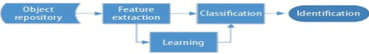
Since digital imaging has become an integral part of research, computer-aided assessment using advanced image analysis has become an important part of many research projects. Model recognition is a scientific research process used to determine the system design models by analyzing the data. The recognition system has emerged with a large accumulation of computer data [8].
cancer, mammography, ultrasonography, and magnetic resonance (MR) images are image-processing-based methods used to provide information [9]. Tumour recognition in the area examined with MR images is usually composed of 2 parts. The first part is the process of selecting the features required for recognition of the tumour or the sizes to be measured. This process is called feature extraction and it is the system feature extractor that performs this operation. Each feature used in tumour detection or the size to be measured is a real number that gives the measurement result. At the beginning of the determining the factors affecting the success of the classification, the selected features should represent all the tumour being sought. The second part of the tumour recognition is classified as benign and malignant, using the obtained feature vectors. In Figure 1, a diagram of tumour recognition system in breast cancer is presented.
Fig. 2 Flowchart of SaELM for classification
III. OBJECTIVE
One major issue of ELM is that it tends to use larger number of hidden neurons than in the traditional gradient descent algorithms.
Moreover, the random initialization of the input weights and hidden biases may affect the performance of ELM.
To solve these drawbacks, global search algorithms such as evolutionary algorithms can be used to experience the best utilisation of ELM.
IV. METHODOLOGY
ELM starts by randomly initializing the input weights and hidden biases and, then in one step, it analytically determines the output weights using MP inverse ( Huang et al., 2006 ). However, due to this random assignment of these weights and biases, ELM usually does not get the optimal values of the weights.
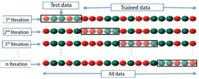
It is important to compare the performance values of machine learning algorithms with a measurable expression and to compare its performances. In this section, we have divided the data set, which is the first criterion affecting the performance of the model and the algorithm used, divided into training and test data, and the second is the identification of performance evaluating expressions.
➢ First criterion: There are various data partition performance evaluation methods such as hold-out and K-fold cross-validation in the literature [13]. The following items should be taken into consideration while distinguishing the data set as training and testing:
The number of samples in the training dataset should be more than the samples in the tested dataset. It is necessary to randomly distribute samples at the distinction of training and test data set.
During the division of the data set into training and test data sets, the target class must include the target data in the distribution of the training and test data sets.
Second criterion: It is necessary to express the performance of the proposed solution for a probing given in machine learning algorithms, or to express how well the algorithm learns. Different evaluation criteria have been developed for this.
Fig. 3 Data set divided into training and test data
V. CONCLUSION
The proposed model is to be experimented based on a medical classification problems using standard dataset. And I will try to recover the experimental results that demonstrate the proposed model can achieve better generalization performance with smaller number of hidden neurons and with higher stability. In addition, it requires much less training time compared to other classification algorithms.
REFERENCES
[1] Akusok, A. , Björk, K.-M. , Miche, Y. , & Lendasse, A. (2015). High-performance extreme learning machines: A complete toolbox for big data applications. IEEE Access, 3 , 1011–1025
[2] Alexandridis, A. , Famelis, I. T. , & Tsitouras, C. (2016). Particle swarm optimization for complex nonlinear optimization problems. In
Proceedings of the 2016 AIP confer- ence: 1738 (p. 480120). AIP Publishing .
[3] Cao, J. , Lin, Z. , & Huang, G.-B. (2012). Self-adaptive evolutionary extreme learning machine. Neural Processing Letters, 36 (3), 285–305 . [4] Chen, W.-N. , Zhang, J. , Lin, Y. , Chen, N. , Zhan, Z.-H. , Chung, H. S.-H. , et al. (2013). Particle swarm optimization with an aging leader
and challengers. IEEE Trans- actions on Evolutionary Computation, 17 (2), 241–258 .
[5] Cheng, R. , & Jin, Y. (2015). A competitive swarm optimizer for large scale optimiza- tion. IEEE Transactions on Cybernetics, 45 (2), 191– 204 .
[6] Cho, J.-H. , Lee, D.-J. , & Chun, M.-G. (2007). Parameter optimization of extreme learn- ing machine using bacterial foraging algorithm.
Journal of Korean Institute of In- telligent Systems, 17 (6), 807–812 .
[7] Das, S. , Abraham, A. , Chakraborty, U. K. , & Konar, A. (2009). Differential evolution using a neighborhood-based mutation operator. IEEE Transactions on Evolution- ary Computation, 13 (3), 526–553 .
[8] Deng, W. , Zheng, Q. , & Chen, L. (2009). Regularized extreme learning machine. In Proceedings of the IEEE symposium on computational intelligence and data mining, CIDM’09, IEEE (pp. 389–395) .
[9] Ding, S. , Su, C. , & Yu, J. (2011). An optimizing BP neural network algorithm based on genetic algorithm. Artificial Intelligence Review, 36
(2), 153–162 .
[11] Gastaldo, P. , Bisio, F. , Gianoglio, C. , Ragusa, E. , & Zunino, R. (2017). Learning with similarity functions: a novel design for the extreme learning machine. Neuro- computing, 261 , 37–49 .
[12] Gori, M. , & Tesi, A. (1992). On the problem of local minima in Backpropagation. IEEE Transactions on Pattern Analysis and Machine Intelligence, 14 (1), 76–86 .
[13] Gupta, J. N. , & Sexton, R. S. (1999). Comparing Backpropagation with a genetic algo- rithm for neural network training. Omega, 27 (6), 679– 684 .
[14] Han, F. , Yao, H.-F. , & Ling, Q.-H. (2013). An improved evolutionary extreme learning machine based on particle swarm optimization.
Neurocomputing, 116 , 87–93 .
[15] Hornik, K. , Stinchcombe, M. , & White, H. (1989). Multilayer feedforward networks are universal approximators. Neural Networks, 2 (5), 359–366 .
[16] Huang, G.-B. , Zhu, Q.-Y. , & Siew, C.-K. (2004). Extreme learning machine: a new learning scheme of feedforward neural networks. In
Proceedings of the 2004 IEEE international joint conference on neural networks, IEEE : 2 (pp. 985–990) .
[17] Huang, G.-B. , Zhu, Q.-Y. , & Siew, C.-K. (2006). Extreme learning machine: Theory and applications. Neurocomputing, 70 (1), 489–501 . [18] Huynh, H. T. , & Won, Y. (2008). Evolutionary algorithm for training compact single hidden layer feedforward neural networks. In