Layered Multicast Recovery
Injong Rhee
y, Srinath R. Joshi
y, Minsuk Lee
y, S. Muthukrishnan
zand Volkan Ozdemir
y,
y
Department of Computer Science
zAT&T Labs-Research
North Carolina State University
180 Park Avenue
Raleigh, NC 27695-7534
Florham Park, NJ 07932
f
rhee,srjoshi,mlee1,vozdemi
g@csc.ncsu.edu
[email protected]
Feb 1999
Abstract
We study the problem of localizing repair packets when packets are lost. When repair packets are multicasted, a highly lossy receiver may swamp the entire multicast “group” with duplicate repair packets thereby wasting bandwidth; thus, the protocols need repair locality.
We present a multicast layering scheme where the sender proactively distributes FEC repair packets among multiple multicast groups. Receivers can selectively tune in to a subset of these multicast groups to obtain number of packets close to the number they require. We develop an efficient algorithm that dynamically determines the optimal distribution of FEC repair packets to a given (small constant) number of multicast groups. The running time of this algorithm is independent of the number of receivers in the multicast session, and is hence highly scalable. However, the optimal algorithm requires the knowledge of the FEC repair requirements of all the receivers in the multicast group, and hence is subject to the implosion problem. To handle the implosion problem, we develop a heuristic algorithm that achieves repair locality very similar to that of the optimal algorithm, but does not require as much global knowledge.
Our multicast layering scheme can be integrated into many known reliable multicast protocols to enhance their scalability. For concreteness, we focus on singly scoped and hierarchically scoped SRM as well as tree-based protocols and present combined protocols incorporating our solutions into each of them. Our simulation experiments suggest that our solutions can substantially enhance the scalability of these reliable multicast protocols.
1
Introduction
Reliable multicast protocols need to address the issue of recovering from packet losses. The crux is to design a protocol that scales to tens of thousands, or even millions of receivers since the added control complexity of multicasting has a greater payoff with such large numbers of receivers. Scalability is thus an important problem in reliable multicasting, and it is a well-studied one. Many clever protocols have been proposed,
e.g., SRM [1], RMTP[2], SHARQFEC [3], TMTP [4], to name a few; the resource web site [5] gives an extensive background.
A natural approach to recover from packet losses is to make the sender retransmit the lost packets to individual receivers. However, such sender-centric retransmission does not scale well. In a large-scale multicast session, the probability that a given packet is lost by some receiver is high; thus, the sender may end up retransmitting every packet. Additionally, if a packet is lost near the sender, most receivers would lose that packet, and it leads to repair traffic that is proportional to the session size. We may avoid this problem by allowing the sender to multicast the retransmission. However, as recent MBone studies [6] indicate, many packet losses are not correlated, and different receivers may experience different loss rates. This leads to the well-known repair-locality problem whereby repair traffic is not localized to its desired receivers. Thus, when retransmission is multicasted, receivers may end up receiving many “unwanted” packets in the repair traffic. Sender-centric retransmission schemes also suffer from the well-known implosion problem in which the sender is potentially flooded by control traffic (request for packets, negative acknowledgment from receivers, status requests, etc).
The popular consensus now seems to be to effectively delegate the responsibility of recovery to the receivers. SRM [1], perhaps the most popular scheme for reliable multicast, allows receivers to multicast requests to the entire group. Any receiver with requested packets can multicast it. With clever use of randomized timers and suppression, SRM effectively solves the implosion problem. Unfortunately, SRM does not solve the repair locality problem. This problem is alleviated, but not entirely solved, by local and hierarchical scoping (grouping of receivers) [7].
There are tree-structured protocols such as TMTP [4], RMTP [2], and LBRM [8] that solve the implo-sion and repair locality problems by imposing a logical tree structure to the multicast sesimplo-sion. Specialized receivers located at the root of the sub-trees of the logical tree receive requests and effect retransmission only to their own children in the tree. These protocols work without any router support, but they need specialized receivers. There are other protocols such as PGMP [9] and LSM [10] which propose to modify the routers in order to localize repair packets to the region where they can be most effective. For these protocols to be effectively used, “special” receivers (or routers) need to be widely deployed. Managing the logical tree involving a large number of specialized receivers under network partition or machine failure would create an enormous administrative burden.
Another approach to solving both the implosion and repair locality problems is to use forward error correction (FEC). This involves splitting the original packet stream into groups ofBpackets, called blocks.
For each block, h FEC encoded packets are generated for suitably chosen h. Receivers can recover the
original block by receiving anyBpackets out of theB
+
hones. When combined with an appropriate ARQtechnique, the FEC technique incurs very low network overhead [11, 12, 13, 14, 15, 3].
To summarize, scoping and employing FEC together with suppression techniques, leads to reliable mul-ticast protocols that are suitably scalable. However, the main issue is to determine how many FEC packets to transmit, and the suitable protocol to schedule the transmission of these FEC packets. Most existing schemes force the sender to multicast as many FEC packets as the most lossy receiver in the session re-quires. This is effective only if all the receivers in the group have similar loss rates. Unfortunately, in most existing protocols, scopes are not defined by the loss rates of receivers, but by their physical locations. In [16, 7], scopes are defined to be receivers within a certain “hop count” or time-to-live (TTL). Administrative scoping incorporated into multicast addresses [17] is also based on physical locations. SHARQFEC [3] also defines scopes based on the physical regions, cities, suburbs, etc. Inevitably, a large scope defined only by physical locations comprises receivers with widely varying loss rates; thus, receivers with low loss rates receive far too many redundant repair packets, and the overall repair traffic is excessive.
Contribution We present a novel protocol called Layered Multicast Recovery (LMR). A multicast session
is allocated with multiple multicast group addresses. The sender multicasts different amounts of FEC pack-ets to different multicast groups. Each receiver joins a subset of the groups that together provide the number of FEC packets it needs under its current loss rate. We present a highly efficient algorithm to find the optimal allocation of repair packets to different multicast groups in order to minimize redundant traffic; its running time is independent of the number of receivers in the session. However, the algorithm requires the source to know the repair requirements of every receiver in the multicast group, and is subject to the acknowledgment implosion problem. To remedy the implosion problem, we develop a heuristic algorithm that achieves simi-lar repair locality as the optimal algorithm in most network topologies, but does not require as much global knowledge. Our two solutions can be employed in various existing reliable multicast protocols to enhance their repair locality, and scalability. In this paper, we integrate our solutions with SRM, a tree-based pro-tocol, and a hierarchically scoped protocol. The resulting protocols are substantially enhanced versions of their original in their scalability.
In what follows, we give a more detailed overview of our contributions.
Layered Multicast Recovery The outline of our protocol is as follows. Within each scope (session, if
there is only one scope), K repair multicast groups (hereafter referred to as repair groups) are allocated.
MLR uses a hybrid FEC/ARQ scheme. First, receivers periodically compute the amount of FEC repair packets required for loss recovery, based on their current loss rates. The basic assumption is that the mean packet loss rate of a receiver does not fluctuate rapidly and slowly varies over time. Given the maximum number of FEC repair packets, f
max
, required by a receiver in the scope, a ZCR (or the sender) partitionsf
max
packets into F=f1
;2
;:::;K
ggroups whereKis given as a some small constant, and transmitsi
repair packets to a different multicast group. While the receiver with the worst packet loss rate joins all the multicast groups to receivef
max
repair packets, others can adjust the amount of repair traffic transmitted tothem by selectively joining only a subset of theKmulticast groups.
Given the number of FEC packets needed by the different receivers, the optimal algorithm allows a ZCR to choose optimalF to minimize the total redundant repair traffic to each receiver in its scope. For instance,
if there are five receivers which require 2, 2, 1, 4 and 4 repair packets respectively, and K
= 2
, then1
and
2
are 2 each in order to minimize the total number of redundant repair packets that all receivers wouldmore than it requires when joining the first repair group.
In this paper, we develop an algorithm determining the optimal F with running timeO
(
U2
K)
whereU is the maximum number of FEC repair packets to add per block. While an unbounded number of repair
packets can be proactively injected, we restrictU to be less than the block sizeBwhich is typically less than
20 (in our simulation, we chose 16). This also limits the total amount of FEC repair packets per block that is received by a member toB. The running time of the algorithm is independent of the number of receivers
in the scope.
However, the optimal algorithm requires to know the number of repair packets required by each receiver (or at least a majority of receivers) to compute the optimal layeringF. This might be a source of feedback
implosion if each receiver periodically reports its repair requirement to the sender. Surprisingly, we find that a simple heuristic algorithm can achieve similar repair locality as the optimal algorithm in most cases where the distribution of loss rates among receivers within a scope is not extremely skewed. The heuristic algorithm does not require the global knowledge of the repair requirements of all the receivers. The algorithm simply multicasts the same number of repair packets to each multicast group, and the number of repair packets is determined by dividingf
max
byK. This scheme calls for keeping track offmax
dynamically. When thefi
of one of the receiveriexceeds the current value off
max
known to all the receivers, it can send the feedbackwith the updated f
max
. Thus it is easy to keep track of the increases infmax
. To keep track of fmax
whenit decreases, we can design a slightly more sophisticated protocol. We do not describe the details of this protocol in this report (details will be provided in the final version). Obtaining f
max
allows an efficient useof feedback suppression where a receiver multicasts its repair requirement if and only if its requirement is less than what it has heard from other receivers in the last epoch period. Similar approach has been adopted in other protocols [18, 19] to reduce implosion.
Organization We review the repair locality problem in Section 2. We present our protocol Section 3.
We present our simulation results in Section 4. There is a rather large body of work related to scalable, reliable multicasting; we discuss some relevant ones in Section 5. We present concluding remarks as well as potential limitations of our work in Section 6.
2
The repair locality problem
The repair locality problem can be best explained using examples. We modified several examples from [3].
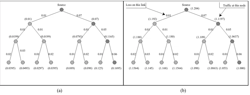
Figure 1(a) shows that a single sender at the root of the multicast routing tree multicasts data to the other nodes which represent the receivers. Branches represent multicast routing paths. Different branches are subject to different loss rates, from low to high rates. The total loss at each node can be calculated by compounding the loss rate of every link between the sender and that receiver. In Figure 1(a), the worst case receiver loses about 17% of the packets.
Source 0.07 0.01 (0.01) (0.07) (0.1165) (0.0793) (0.0199) (0.0199) (0.1695) (0.125) (0.089) (0.098) (0.0395) (0.0297) (0.0493) (0.0395) 0.06 0.01 0.02 0.01 0.02 0.01 0.03 0.02 0.01
0.01 0.01 0.05
Source (1.204) 0.07 0.01 (1.192) (1.1197) (1.0637) (1.109) (1.180) (1.180) (1.000) (1.053) (1.098) (1.0863) (1.1564) (1.168) (1.145) (1.1564) 0.06 0.01 0.02 0.01 0.02 0.01 0.03 0.02 0.01
0.01 0.01 0.05
Traffic at this node Loss on this link
(a) (b)
Figure 1: (a) A multicast tree (the number in parentheses near a node represents the loss rate of that node), (b) Normalized traffic volume for non-scoped and non-layered FEC.
(a) (b) Source (1.0752) 0.07 0.01 (1.0645+0) (1.000+0.0526) (1.000+0.0638) (1.042+0) (1.054+0) (1.054+0) (1.000) (1.0532) (1.032) (1.021) (1.033) (1.043) (1.022) (1.033) 0.06 0.01 0.02 0.01 0.02 0.01 0.03 0.02 0.01
0.01 0.01 0.05
Traffic at this node including newly added FEC traffic
Source (1.000+0.010+0.0652) 0.07 0.01 (1.0+0.01+0) (1.000+0.01+0.0426) (1.000+0.01+0.0538) (1.000+0.01+0.011) (1+0.01+0.011) (1+0.021+0.010) (1.000) (1.000) (1.000) (1.000) (1.000) (1.000) (1.000) (1.000) 0.06 0.01 0.02 0.01 0.02 0.01 0.03 0.02 0.01
0.01 0.01 0.05
Traffic at this node including newly added
FEC traffic on two multicast groups
Figure 2: (a) SHARQFEC with normalized traffic volume, (b) LMR with normalized traffic volume 1.
be much larger.
Figure 2(a) shows a scoped version (SHARQFEC) of the same scenario as the above. The ZCRs (i.e., internal nodes and the sender in the figure) of nesting scopes inject sufficient repair packets to satisfy the receiver with the highest loss rate among its children. The amount of redundant packets is greatly reduced because of scoping. However some receivers (especially the ones in the left side of the tree) are still subject to a significant amount of redundant traffic (about 6.4%). This scenario is quite real. Since a single scope can expand to include many receivers (e.g., five hundred receivers as proposed in [3]), it is highly unlikely that the receivers in the same scope have similar loss rates. Therefore, scoping alone is not adequate for solving the repair locality problem.
Figure 2(b) shows the result when LMR is applied to scoping assuming each ZCR can have two repair groups. The label
(
x+
y+
z)
at each internal node denotes the normalized amount of trafficxthat it getsnormalized amountz of the FEC traffic it adds to the second repair group. Each receiver has a choice of
joining one or both groups. Under the current scenario, every node receives no more than what it requires to recover from its own losses. This example suggests that with a few additional multicast groups and appropriate assignment of the number of repair packets sent to each repair group, we can substantially reduce the redundant repair traffic. In the following sections, we develop and formalize the LMR protocol in greater depth.
3
A single scoped LMR protocol
We first sketch the outline of LMR for a single scope where the sender is the only node that can proactively multicast FEC repair packets. Then we show how it can be integrated with SRM [1] and a tree-based protocol such as RMTP [2].
3.1
The outline of the protocol
The sender has a fixed number of multicast groups g
0
;g1
;:::;gK
, where K is a small constant. K istypically less than B, where B is the number of packets in a block. The sender multicasts data blocks to
multicast groupg
0
, which we call the base group. The other multicast groups are repair groups.Depending on the number of multicast groups allocated to the sender, the protocol runs in one of two modes: static or dynamic. Typically, if K is larger than B=c wherec is a small constant and a protocol
parameter, it chooses the static mode; otherwise, it is in the dynamic mode. The mode of LMR is determined at the beginning of the session.
In the static mode, the sender always transmits
i
=
dB=KeFEC repair packets to groupgi
. If there aresufficiently many repair groups, the sender can transmit the groups of repair packets in a fine granularity; hence, the redundant traffic is minimal. For example, when KB=
2
, each receiver gets at most one morerepair packet per block than it requires since at most two repair packets can be sent to each repair group. The added benefit of dynamically allocating different amounts of repair packets to the repair groups is minimal. Note that in the static mode, the sender does not need to know how many repair packets receivers require, so no feedback is necessary.
In the dynamic mode, based on feedback from receivers indicating information on the number of repair packets they need, the sender determines the number of repair packets to send to each group. Each Each receiver iperiodically estimates the number of repair packets it needs, denoted f
i
. fi
is computed basedoni’s mean loss rate. The loss rate is estimated through simple exponential weighted moving average; this
estimation is based on the assumption that persistent loss rates tend to vary slowly.
The goal is to determine the optimal distribution of repair packets among repair groups. Let
j
be thenumber of repair packets to be sent to repair groupg
j
.j
’s are chosen so as to minimize total (equivalently,the average) number of redundant repair packets sent to receivers. We discuss the algorithm to compute
j
in Section 3.3. To compute
j
, the sender keeps statistics on repair packet requirements of receivers, basedon feedback received from a set of receivers. The discussion on how feedback is sent is given in Section 3.4. The statistics are used to determine the optimal distribution of repair packets among repair groups. Let
j
be the number of repair packets to be sent to repair group gj
. Initially, when the sender does not haveThe sender includes the information about the distribution of repair packets in each packet it sends out. We call this the repair group information (RGI). In the static mode, RGI needs to occupy only one octet to store B=K because all repair groups carry the same number of repair packets. In the dynamic mode, a
data packet needs to includeK numbers, each indicating the number of repair packets to be sent to a repair
group (i.e.,
j
’s). Typically, in the dynamic mode,Kis less thanB=2
. Thus, these numbers may occupy uptod
log
2
(
B=2)
eB=2
bits. For example, forB= 16
, this requires only three octets to store the8
numbers.We assume that the transmission rate of data and repair packets is governed by a flow and congestion control mechanism which is outside the scope of this paper.1 The overall transmission sequence works as follows. The sender multicasts the data to the base groupg
0
. Immediately after that, the sender multicastsa group of
j
FEC encoded repair packets togj
, in increasing order ofj’s. Two consecutive repair packetsare delayed by
f
units of time in order to reduce the effect of burst losses (in our simulation, we set it to three packet intervals). The rationale behind this scheme is that the transmission rate of the sender must be about the same as that in non-layered hybrid ARQ protocols.Based on the latest RGI, a receiveridecides to be in a subset of repair groups as described below. It
always belongs to the base groupg
0
. Then it finds the minimumr,r K, such that the sum of1
tor
isat least as large asf
i
, and joins multicast groupsg1
;g2
;:::;gr
. Thus if a receiver joinsgj
, then it has to joingroups from g
1
togj
?
1
. Since repair packets ing
k
;1
k K?1
are always transmitted before those in gk+1
, this rule allows receivers to recover from losses as soon as possible. This is the layering aspect of ourprotocol.
If the number of packets lost per block (including data and repair) by a receiver is larger than the incoming repair packets from its current repair groups, then the packet losses are irrecoverable. In that case, the receiver initiates a request for additional transmission of FEC repair or data packets from the sender or other receivers who recover the same block. The specifics of how this request is handled depends on the type of reliable multicast protocols being integrated with LMR. We discuss this issue in detail when we explain how the LMR protocol can be combined with SRM and a tree-based protocol in Sections 3.4 and 3.4.1 respectively.
3.2
Layering Algorithms
We first describe the optimal algorithm, and then describe a heuristic algorithm for determining F that
minimizes the redundant traffic sent to all receivers.
3.2.1 Optimal layering
Formally our problem is as follows. We have nreceivers; the ith receiver has a demand f
i
1
(of FECpackets). Say
max
i
fi
U. We are given a parameter K which is the number of repair groups. Our goalis to choose
1
;2
;:::;K
,i
1
. Here,i
is the number of FEC packets sent to the multicast groupiby the sender. All
i
’s andfi
’s are integers. Each receiver ijoins the multicast groups1
;;j such that P`=j
`=1
`
fi
andjis the smallest integer with this property. The cost for theith receiver is(
P`=j
`=1
`
)
?fi
,wherej is as above, and the total cost is the sum of the cost for each receiver. The problem is to find the
solution (
i
’s and their ordering1
;:::;K
)
of minimum total cost.1
We observe that although the session sizenis large,U is substantially small; typicallyU
20
. Kisalso small as described earlier.
To some extent, this problem is related to the k-median problem and, more generally, to the facility
location problems in the literature, both of which are mildly hard, to notoriously hard not only to solve exactly in polynomial time, but even to approximate. They have been a subject of intense study even recently in the Theoretical Computer Science community [21]. The focus there is on the case whenU is
much larger thannand the distance function betweenf
i
’s is fairly sophisticated; in our problem, nis verylarge compared toU and the distance function is simple. Here, we are able to show that our problem can be
solved optimally in running time which is a small polynomial inU andK, independent ofn.
It suffices to consider the problem of finding the cost C in the optimal solution – recall the definition
of the cost from earlier. A particular solution of
i
’s with this cost C can be easily retrieved from ourdescription below.
For now, let us consider the subproblem in which our goal is to find the optimal solution using`repair
groups for receivers which request at most iFEC packets, that is,f
j
’s,1
fj
iU. Say this solutionis
1
;;`
. We denote its cost byS(
i;`)
and denote Pj=`
j=1
j
bySS(
i;`)
. Note thatSS(
i;`)
is the totalnumber of FEC packets sent out by the sender since it sends
j
packets over thejth multicast group if wesolve this subproblem alone. The following observation, although simple, proves to be the key. Informally, it says that the number of FEC repair packets sent by the sender over all the multicast groups
1
;:::;`,while solving this suproblem optimally equals the maximum number of FEC repair packets requested by any receiver which requested no more thanipackets. Formally,
Lemma 3.1 For any`,SS
(
i;`) = max
h
fh
wherefh
i.Proof Sketch. We fix a value of `and showSS
(
i;`) = max
h
fh
wherefh
i; that suffices. Trivially,SS
(
i;`)
max
h
fh
, fh
i. Therefore, it suffices to prove SS(
i;`)
max
h
fh
, fh
i. Assumeotherwise; thus, the optimal solution
1
;2
;:::;`
,k
ifor1
k `, hasSS(
i;`)
>max
h
fh
wheref
h
i. Consider the solution1
;2
;:::;`
?1
,k
ifor1
k `. This too is clearly a valid solution,but we can quite easily argue that this has strictly smaller total cost than our optimal solution. Thus we derive contradiction to our assumption.
Henceforth, we letSS
(
i)
denoteSS(
i;`)
for any `. From our observation above, SS(
i) = max
h
fh
wheref
h
i. We have the following recurrence:S
(
i;`) = min
j
j1
j<i
S
(
j;`?1) +
C(
j+ 1
i?1)
;where C
(
ab)
is the total cost of all u’s such that a fu
b. It is easy to see that C(
ab) =
Pa
f
ub
(
SS
(
b)
?fu
)
. In order to solve our problem, it suffices to computeS(
U;K)
.We computeS
(
U;K)
using dynamic programming. We initialize an array S[1
U;0
K]
such thatS
[
i;0] =
1andS[
i;j] = 0
forijand1
j K. Also, S[
i;1] =
C[1
;i?1]
for alli. Now for each2
`K, we consider each choice ofiand we calculateS[
i;`]
using the equation above.Say the time taken to determineC
(
ab)
for anya;bis at mosttQ
. There areO(
UK)
terms of the formS
(
i;`)
each of which takes timeO(
UtQ
)
to compute. The total running time is thusO(
U2
KtQ
)
. We cannaively upper boundt
Q
to beO(
U)
by computingC(
ab)
whenever needed. A more efficient solution isLemma 3.2 We can compute C
(
ab)
for all a;b in time O(
U2
)
after which we can determine anyC
(
ab)
in timetQ
=
O(1)
.Proof. We compute the tableZ
(
a;b) =
C(
ab)
for alla;bwhich can be looked up when needed inO(1)
time. In order to computeZ
(
a;b)
, we determine tablesX(
a;b) =
SS(
ab)
andY(
a;b) =
Pa
f
ub
fu
for each a;b. Both the tablesX andY can be easily computed inO
(
U2
)
time. We then use the followingformula:
Z
(
a;b) =
C(
ab) =
Xa
f
ub
(
SS(
b)
?fu
)
=
Xa
f
ub
SS
(
b)
? Xa
f
ub
f
u
=
X(
a;b)
?Y(
a;b)
Thus it takesO
(
U2
)
time to compute theZ table.Based on the arguments above, we have our main result:
Theorem 3.3 The optimal solutionS
(
U;K)
can be determined in timeO(
U2
K)
.We make several remarks about our result. (1) In order to determine the set of
i
’s in the right order withthe optimal costS
(
U;K)
, we store indexjwhere the minimum occurs in the formula forS[
i;`]
. Using this,we can determine the set
i
correctly and efficiently (as is standard in dynamic programming solutions). (2)We can provide a more sophisticated algorithm that is theoretically more efficient than one we have stated above. But for our implementations, the above solution suffices. (3) Our solution above applies to many other cost functions such as minimizing the maximum of
(
P
`=j
`=1
`
)
?fi
over all receivers.3.2.2 Heuristic layering
The sender needs to know the repair packet requirements of every receiver to compute optimal layering, and thus, requires feedback from every receiver. As the number of receivers increases, feedback implosion limits the scalability of the protocol. To avoid feedback implosion, we resort to heuristics to computeF that
effectively reduces redundant traffics sent to receivers. We use the performance of the optimal algorithm as a yardstick to gauge the performance of the heuristics.
Many heuristics are possible. In this paper, we present a simple algorithm where the sender obtainsf
max
from receivers, and sends df
max
=Kerepair packets to each repair group. We can obtain the current fmax
without causing implosion as follows. This scheme calls for keeping track of f
max
dynamically. Whenthe f
i
of one of the receiver iexceeds the current value of fmax
known to all the receivers, it can sendthe feedback with the updated f
max
. Thus it is easy to keep track of the increases infmax
. To keep trackoff
max
when it decreases, we can design a slightly more sophisticated protocol. We do not describe thedetails of this protocol in this report and only describe the case when f
max
increases. The protocol runsbased on rounds. At each round, the sender multicasts a report message. Receiving the report message, each receivericomputesf
i
, and sets its timer to a random value within[0
;Dmax
?Ds;i
]
whereDmax
is thecurrent maximum one delay from a receiver to the sender, andD
i;s
is the current delay from receiverito thesender. When the timer expires, the receiver multicasts a feedback message containing f
i
if and only if itf
i
received within time period Dmax
after sending the report message. Note that it is possible to computedelays between every pair of receivers [22] in a scalable fashion. For more information, please refer to [22].
In this algorithm, receivers are subject to no more than df
max
=Ke?1
repair packets (if the same lossrate persists). The performance of the algorithm degrades when the distribution of loss rates within a scope is highly skewed between 1 andf
max
. For instance, while one receiver requires 16 repair packets (note thatf
max
cannot be bigger thanB), the rest of receivers requires one repair packet. IfK (the number of repairgroups) is two, then all other receivers will be subject to 7 redundant repair packets per block. However, the performance improves linear toK. In the above example, ifK
= 4
, then the maximum redundant packetsreduce to 4 packets.
3.3
Determining the number of FEC repairs required by a receiver
The number of FEC packets that a receiver needs depends on the pattern and rate of its losses. We adopt the standard model for packet losses found in the literature [23, 14, 11]. The data packet losses are assumed to undergo burst losses. Hence, they are described by a two-state model: one state (referred to as state 1) represents a packet loss, and the other state (referred to as state 0) represents the successful receipt of the packet. If the system is in state 0, the probability of staying in state 0 is, and the probability of switching
to state 1 is
1
?. If the system is in state 1, the probability of staying in state 1 is and the probabilityof moving to state 0 is
1
?. Both parameters and can be obtained from the measured mean lossrate and burst length. Each FEC packet belonging to the same block is separated by
f
time distance.f
is set large enough to force the losses of FEC packets to be close to independent. It was reported in [23] that periodic UDP packets separated by as little as 40 msec tend to undergo near-independent losses. Thus, we assume that FEC repair packets undergo independent random losses; hence, they are described using a binomial distribution; again, the independent loss probability is known from measurements. The losses of data packets (in multicast group0
) and those of FEC packets are assumed to be independent.We can calculate the following two quantities efficiently. LetP
(
f;i)
denote the probability of receivingj packets out off FEC repair packets; it can be computed in a straightforward way from the definition of
the binomial distribution. LetD
(
B;i)
be the probability of receivingidata packets out of a block ofBdatapackets under the two-state model. D
(
B;i)
can be computed using dynamic programming in timeO(
B2
)
using the recursive definition ofDin [14].
Two parameters are relevant. The first is, the probability of recovering a block when the total number
of repair packet in the multicast groups the receiver belongs to is f. That is, if i packets are received
from the base group, at least
(
B?i)
FEC packets are needed from the repair groups in order to recoverthe block. Thus,
=
PBi=max(B
?f;0)
D
(
B;i)
Pf
j=B
?i
P
(
f;j)
. The second parameter of relevance is the expected wasted bandwidth due to redundant FEC repair packets. Let EX
(
B;f)
be the expectednumber of packets received when f FEC packets are used to protect B data packets. It is easy to see
that EX
(
B;f) =
PBi=0
iD(
B;i) +
Pf
j=0
jP(
f;j)
. Then, the normalized expected bandwidth wastage is EW(
B;f) =
EX(B;f)
?B
B+f
.One approach to estimate the FEC repair packets for a receiver would be to set very close to 1; that
would give a value forf. This approach requires FEC repair packets to protect transmission even from very
0.00 0.05 0.10 0.15 0.20 0.25 Normalized Expected Bandwidth Wastage
0.5 0.6 0.7 0.8 0.9 1.0
Probability of recovery
loss rate = 1% loss rate = 5% loss rate = 10% loss rate = 15% loss rate = 20% loss rate = 25% loss rate = 30%
In this region there is significant improvement in probability of recovery while bandwidth wastage is around 5%−6%.
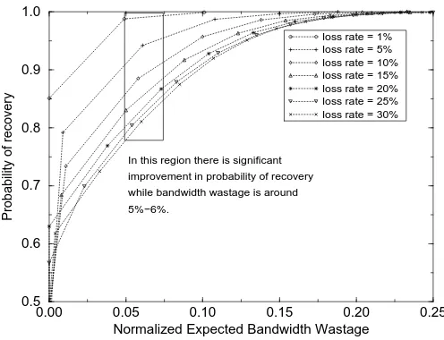
Figure 3: The relation of wasted bandwidth and the probability of recovery whenB
= 16
.the probability of recovery given the expected wasted bandwidth is bounded by an acceptable amount for a receiver. Since different receivers may be able to tolerate different amounts of wasted bandwidth, this approach would allow receivers to wage their own “risk” in getting FEC repair packets. In our simulations, we set the tolerable wasted bandwidth to be 5% of the total forward bandwidth.
The effect of the number of FEC packets on the wasted bandwidth and probability of recovery is shown in Figure 3. We calculatedandEW
(
B;f)
withB= 16
while varyingf and loss rates. The plot shows thatwhen the normalized expected bandwidth wastage is around 5%-6%, the chances of recovery are significant. Note that the chances of recovery can be up to 20% higher than the case when the bandwidth wastage is minimum.
3.4
Integrating with SRM
Request. When a receiverrfails to recover a block, it sets its request timer in the same manner as specified
by the SRM protocol. That is, the delay is chosen uniformly from the interval
2
i
[
C1
dS;r
;(
C1
+
C2
)
dS;r
]
,where C
1
are C2
are protocol parameters typically set to2
; here, dS;r
is the receiver r’s estimate of theone-way network delay time from the sender (S) tor during a multicast, andiis the backoff factor, which
is described below. When the timer expires, it multicasts a request for FEC repair packets for its incomplete block. The number of repair packets requested is a tunable parameter that depends on the receiver’s past experience on the number of duplicate repair packets, denoted d, it gets for each request. If a receiver
requiresypackets, then it may requestdy=xerepair packets. If the receiver receives a request from another
receiver for the same block before the timer expires, it increments its backoff factoriby one, and resets the
request timer.
Repair If receiver r receives a request from receiver q for n
q
packets from a block r has successfullyrecovered, it sets its repair timer to
[
D1
dr;q
;(
D1
+
D2
)
dr;q
]
where D1
and D2
are set to 1, and dr;q
isthe estimated network delay from r toq. We associate with the repair timer for r, a numberN
r
which isthe number of repair packets it would send when the timer expires. N
r
is initialized to nq
which is therequested number of repair packets. If it receives further requests for repair packets, N
r
is updated to thenew requested value if that is larger. If it receives a repair packet from another receiver while the timer is on, N
r
is decremented by one. This is the technique used in SHARQFEC [3] for suppressing request andrepairs.
When the timer expires andN
r
>0
,rmulticastsNr
repair packets selected as follows. First, the nodegenerates
(
F+ 1)
Nr
unique FEC-encoded repair packets whereF is a tunable parameter chosen based onthe size of a block and the computational overhead in generatingF FEC repair packets (in our simulations,
we set it toB, the block size). Then, it randomly choosesN
r
packets from packets with sequence numberbetweenF and
(
F+ 1)
Nr
. This scheme increases the chance that receivers will get unique FEC-encodedrepair packets. Note that the sender would not transmit more thanBrepair packets, and every node uses the
same FEC-encoding scheme.
3.4.1 Integrating with a tree-based protocol
LMR can be combined with a tree-based protocol such as RMTP[2] or LBRM[8]. As discussed in the introduction, a tree-based protocol solves implosion and repair locality by imposing a logical tree structure, and designating a receiver — called the designated receiver (DR) in RMTP — as the root in the sub-trees of the tree.
A tree-based protocol can benefit from LMR. Because LMR multicasts FEC-repair packets, FEC repair packets can proactively suppress many repair requests. In addition, since LMR allows receivers to choose the amount of FEC repair packets to receive proactively, it reduces much of the repair locality problem. Since the implosion and repair locality problems become less limiting by the use of LMR, the tree-based protocol can scale to incorporate a larger fanout, resulting in a reduced number of DRs.
protocols, DRs actually unicast repair packets to their child receivers [2] when there are not many requests for the same packet pending. When packets are unicasted, the repair locality problem is not the key concern.
The tree structure of the protocol actually simplifies aspects of LMR e.g., in gathering feedback, and by decreasing the sender’s load in processing feedback from receivers. A DR can gather feedback, compile the statistics on the number of receivers in its subtree and the required number of repair packets, and report that to its parent DR. Thus the sender receives only a small number of feedback messages from its children.
4
The hierarchically scoped LMR protocol
The preceding discussion of LMR protocol focused on the single scope case where the sender is the only node proactively injecting FEC repair packets. LMR can also be applied to hierarchically scoped protocols such as scoped-SRM [1] or SHARQFEC [3]. Hierarchical scoping is in general effective in localizing repair, thereby scaling reliable multicast to large number of receivers. The combination of LMR and hierarchical scoping can substantially increase this scalability.
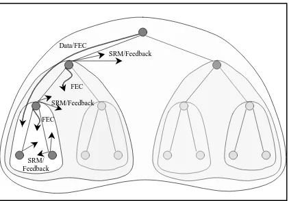
In this section, we describe how LMR can be used in presence of scoping. Informally, this can be achieved by electing scope leaders in each local scope, and letting scope leaders proactively distribute FEC repair packets to different local multicast groups based on the feedback received from their own scopes. Receivers can listen to a set of local multicast groups to receive repair packets. There are many details and we describe them now.
4.1
Hierarchical Scopes
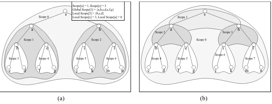
The entire multicast group is divided in to scopes as shown in Figure 4. Each scope is given a unique scope ID. Every scope except scope 0 has one parent scope, and may have one or more child scopes. Each scope designates the node closest to the sender to be the representative of the receivers in that scope; this representative is called the Zone closest receiver (ZCR). The sender becomes the ZCR of the scope 0. A receiver can be a member of one or more scopes. For instance, the ZCR of a scope is also a member of its parent scope. The dynamic election of a ZCR within a scope is described in detail in [3]; we adopt that procedure and do not describe it here any further.
Definitions. The following definitions are helpful in describing our protocol. The scope of a receiverris
iifris a member ofiand there does not exist a scopej 6
=
iof whichris a member, such thatjis a childscope ofi. Thus, in Figure 4, a’s scope is
1
whilec’s scope is3
. The global scope of a scopeiincludesevery receiver that is a member of scope i. For example, in Figure 4, the global scope of
1
includesa,b,c, and d. The local scope of a scopeiincludes only those receivers whose scope isi(i.e., those belonging
only to scopei). For example, in Figure 4, the local scope of
1
contains onlyaandbwhich are the ZCRs ofthe child scopes of scope
1
. The local scope of a receiver is the scope of that node if that receiver is not the ZCR of the scope. Otherwise, it is its parent scope. Thus, the local scope ofcis3
while the local scope ofais
1
.c
a a
c d
b e
f g j k
i h
l
m n
s
Scope 0
Scope 1 Scope 2
Scope 3 Scope 4 Scope 5 Scope 6 Scope[a] = 1, Scope[c] = 3 Global Scope[1] = {a,b,c,d,e,f,g} Local Scope[3] = {b,c,d} Local Scope[c] = 3, Local Scope[a] = 0
d f g
b e
s
h
i l
j k m n
Scope 1
Scope 2 Scope 3
Scope 4 Scope 5
Scope 6
Scope 7 Scope 0
(a) (b)
Figure 4: (a) Nested Scopes, (b) Non-nested scopes
descendent scope. All the non-ZCR receivers in a non-nested scopeibelongs to only scopesiand 0. Thus,
in a non-nested scopei, its global and local scopes are the same. Figure 4 shows examples of non-nested
and nested scopes respectively.
4.2
The allocation of multicast groups
Each ZCR is allocatedK
+ 1
unique multicast groups. The number of multicast groups allocated to eachZCR is determined at the beginning of data transmission based on the expected sizes of multicast groups and scopes. In each scope x, there are g
x;0
;gx;2
;:::;gx;K
multicast groups. We call gx;0
the base groupof scope x. The sender multicasts data packets to g
0;0
and all receivers join that group. Each receiver is amember of the base group of its own scope. ZCRs are members of the base group of the parent scope of their scopes. A local scope iis allocated one multicast group, called local groupl
i
, which comprises allreceivers whose local scope isi, and the ZCR of scopei. The local groups are used for the dissemination of
the feedback, and for retransmission request and repair packets.
Each ZCR is responsible for multicasting FEC repair packets to its scope. Each ZCR at scopex
mul-ticasts FEC repair packets to multicast groups g
x;1
;:::;gx;K
. Whether a scope is nested or not affects theLMR protocol (especially, that of receivers and ZCRs). We discuss the LMR protocols for non-nested scopes and nested scopes separately.
4.3
Non-nested scopes
Each receiver multicasts its feedback only to its local group and the feedback is identical to that in the single scoped protocol.
Data/FEC
Feedback SRM/
FEC
FEC
SRM/ Feedback
SRM/Feedback
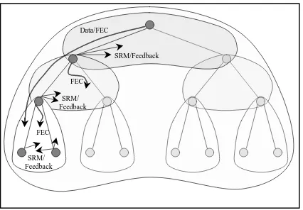
Figure 5: The extent of the multicasted information travels in non-nested scopes
successfully receives each block of data, it multicasts
i;j
,1
j K, of uniquely FEC encoded repairpackets tog
i;j
. As before, there is a delay between successive FEC pockets in order to reduce short burstlosses of FEC repair packets. The ZCR multicasts its session information (i.e., the information on the distribution of repair packets) to its base group and includes it in every repair packet it multicasts. The ZCR participates in the network delay estimation protocol for the receivers of its local scope by multicasting acknowledgment to probes (included in feedback) received from its local group.
Receivers behave much the same way as they do in the single scoped protocol. A receiver in scope x
always obtains data packets fromg
0;0
and the session information fromgx;0
. Using the session information,a receiver finds the minimumr,r k, such that the sum of
x;1
tox;r
is at least as large as its currentlyrequired number of repair packets. It then joins multicast groupsg
x;1
;gx;2
;:::;gx;r
for FEC repair packets.Figure 5 depicts the extent of the multicasted information travels in non-nested scopes. Arrows crossing over two scopes indicate that information is multicasted to both scopes, and arrows contained in a scope indicate that information is multicasted only to that scope. Data packets are multicasted to every scope while FEC repair packets, retransmission requests and repairs are confined to local scopes.
4.4
Nested scopes
A scope can be nested in multi-levels. The nesting level of a nested scope iis the number of scopes
con-taining scopei. We assume that if any two scopesjandknest scopei, either scopejnests scopekor vice
versa. Note that the global scope of the parent of a nested scope is different from the local scope of the parent because a receiver.
As in non-nested scopes, receivers multicast feedback only to their local repair group, and based on the feedback, the ZCR of that scope determines the number of FEC repairs that it proactively transmits to its global scope. This number also depends on how many repairs it receives from its nesting-ancestor scopes. Figure 6 depicts the extent that messages travel to in nested scopes. While FEC repair packets multicasted to global scopes, retransmission requests and repairs, and feedback multicasted only to local scopes.
Letf
A
be the number of FEC repairs needed by a receiver A. Suppose that the scope of the receiveris nested by t scopes, s
1
;s2
;:::;st
(i.e., the nesting level is t), s1
is the scope of receiver A, and sj
,2
j n, contains sj
Data/FEC SRM/Feedback FEC FEC SRM/Feedback SRM/ Feedback
Figure 6: The extent of the multicasted information travels in nested scopes
scopes. The receiver always listens to all the base groups of its nesting scopes. The RGI of a scope also is transmitted to its base group as well as included in every repair packet that the ZCR of that scope multicasts. Let
x;y
;y1
be the number of FEC repair packets to be transmitted to multicast groupgx;y
.It is nontrivial to determine the multicast groups that a receiver must belong, for obtaining the repair packets. A receiverAin scopes
1
first takes into account the number of repair packets that the ZCRs of itsnesting scopes expect to receive from their own ancestor ZCRs. This is because a receiver may have lower loss rates than its ZCR; this happens sometimes when the ZCR is not at the routing path from the sender to that receiver. Since a ZCR can inject repair packets for a block only after it successfully receives that block, when the ZCR has higher loss rates than a receiver. relying on repair packet from that ZCR would prolong recovery delay for that receiver. In what follows, we sketch a more sophisticated protocol for determining the multicast groups to which a receiver belongs.
LetR
s
j,1
jlen, be the number of FEC repair packets that the ZCR
s
j expects to receive from its
own nesting ancestor scopes. R
s
jis part of the session information thatZCR
s
jmulticasts. Based on the
R
s
j’s, receiver
Adetermines the expected number of repair packets E
s
j to receive from each ZCR
s
j. E
s
j
is determined as follows. Lets
x
be the smallest scope such thatfA
?Rs
x is positive. We set E
s
i
= 0
for1
ixandEs
x=
f
A
?Rs
x. For each scope
s
r
,x+1
r n?1
, find the smallest nesting scope ofsr
, sl
, (l>r) such thatRs
l ?R
s
r is positive. Then we set E
s
i
= 0
forr ilandE
s
l+1=
R
s
l?R
s
r. Werepeat the above process until we reach the largest scope (s
n
= 0
). Then we setE0
=
R1
ifR1
is positive,andE
0
= 0
otherwise. For each scope sj
for whichEs
j>
0
, receiver Afinds the minimumr such thatjoiningg
s
j;1
;:::;g
s
j
;r
gives at least Es
j repair packets, and it becomes a member of those groups.
If a scope iis in the static mode, its ZCR distributes B=K repairs to each g
i;j
,1
j K. If thescope is in the dynamic mode, it uses the following algorithm. The ZCR first determines the number of FEC repairs it would get from its nesting scopes. Let
i
be that number, andfmax
be the maximum number ofrepairs required by receivers in its local scope. The ZCR multicasts at mostf
max
?i
repair packets to itsrepair multicast groups. The algorithm in Section3.2.1 determines the distribution of these repair packets to its repair groups.
Examples. Figure 7 shows two examples for the calculation ofE
i
, the expected number of proactive repairfA = 6
R1 = 2
R2 = 8
R3 = 6
Scope 0
Scope 2
Scope 3 Scope 1
E3 = fA-R3 = 0 E2 = 0 (R3 > R2)
E1 = R1-R3 = 4 E0= R1 = 2
ZCR0 = Sender
ZCR1
ZCR2
ZCR3
A fA = 10
R1 = 2
R2 = 3
R3 = 4
Scope 0
Scope 2
Scope 3 Scope 1
E3 = fA-R3 = 6 E2 = R3-R2 = 1
E1 = R2-R1 = 1 E0= R1 = 2
ZCR0 = Sender
ZCR1
ZCR2
ZCR3
A
(a) (b)
Figure 7: Examples on computingE
i
.than their ZCRs whereas Figure 7(b) shows a different scenario where receivers may have lower loss rates than their ZCRs. For simplicity, we assume that ZCRs are in the static mode andb=K
= 1
which meansthat only one repair packet is transmitted to each multicast group. In Figure 7(a),R
1
= 2
;R2
= 3
;R3
= 4
,andf
A
= 10
. According to the equations discussed above, receiverAsetsE3
= 10
?4 = 6
,E2
= 4
?3
,E
1
= 3
?2
, andE0
= 2
. Thus, the sum ofEi
’s for receiverAis 10. In Figure 7(b),R1
= 2
;R2
= 8
;R3
= 6
andf
A
= 6
. HereR3
is less thanR2
. AlsoE3
= 6
?6 = 0
. SinceR2
>R3
,E2
= 0
, andE1
=
R1
?R3
= 4
because scope 1 is the smallest scope that has the expected number of packet from its ZCR (R
1
) to be smallerthan R
3
. E0
= 2
. Thus, the sum ofEi
’s for receiverA is 10. Note that receiverAdoes not receive anypacket fromZCR
2
andZCR3
because they have the same or worse loss rates. Thus, the recovery of blocksreceived by receiverAdoes not depend on those ofZCR
2
andZCR3
.4.5
Retransmission in scopes
When a receiver cannot recover a data block from receiving FEC repairs, it asks for additional transmission of FEC repair packets from other receivers within its local scope in the same way it was described in Section 3.4. But determining the time to send a request in a nested scope is not trivial. In the single scoped protocol, it can be determined by detecting gaps in the sequence numbers of packets because repairs are transmitted in a sequential order. For instance, the sender always multicasts in each repair group the FEC repair packets of a block before those of the next block. When listening to a repair group, it never receives the repair packets of earlier blocks if no reordering of packets happens in the network. Thus when a receiver gets a repair for a block before receiving a repair for its previous block, it can safely assume that it lost that repair. Unfortunately, this does not work in nested scopes because ZCRs can only transmit repair packets of a block only after they recover that block, and may recover blocks in different orders than they are transmitted. Thus, even if it receives a repair for a block before a repair for the previous block, it cannot decide whether that packet is lost or has not been sent.
To handle this situation, for each repair group that it joins, a receiver a estimates the expected time
repair group y, it computes the expected arrival timet
a;y
of all ofxrepair packets relative to the receivingtime of the first packet in that block. t
a;y
can be computed by addingxf
andtb
, the expected time thatits ZCRbrecovers all the packets in the block relative to the receiving time of the first packet. The expected
time that receiver brecover all of its packets in the block can be computed by taking the maximum of the
expected arrival time for every repair group it listens to. ZCRbincludest
b
in its RGI so that receiveracancomputet
a;y
.When a receiverareceives a data packetiof a block whereiis the sequence number of the packet within
that block, andiis the first packet it receives in that block, it sets its timer, called recovery timer, for a repair
group yto
(
b?i)
packet interval+
ta;y
+ 2
sd, wheresd is the standard deviation in delays fromZCRbtoa. If it does not receive allxpackets from that ZCR, it considers that those packets it have not
received are lost. When a receiver detects a packet loss from which a data block cannot be recovered even if it would receive all FEC packets it is supposed to receive from all of its currently joined repair groups, it sets its request timer to be a random number within
2
i
[
C1
dZ;a
;(
C1
+
C2
)
dZ;a
]
wheredZ;a
is the delayfrom the ZCRZofa’s local scope to itself. While the request timer is pending, if it receives a repair packet
that it considered lost (for instance, due to wrong estimation of expected recovery), it cancels the request timer. Even if receiving that packet, and any repair packets following it in the future does not recover their pertaining block, it sets the request timer again.
When its request timer expires, receiversamulticasts a request to its local group ifais not ZCR. Ifais
a ZCR, then it multicasts it to its parent’s local group. When a receivercgets a request, it sets its timer to be
a random number within
[
D1
da;c
;(
D1
+
D2
)
da;c
]
.4.5.1 Nesting vs. Non-nesting scopes
Nested scopes allow receivers to receive repairs from outer scopes, and therefore, there is more chance of recovery than non-nested scopes. A receiver does not have to rely only on the ZCR of its scope to receive FEC repairs. Since it is possible that that ZCR may not be in the routing path and experiences more losses than its child receivers, a receiver can rely on other ZCRs of its nesting scopes for FEC repairs. The protocol described in Section 4.4 handles this automatically. Note that a ZCR injects repairs only when repairs required to recover its losses are not enough to recover its child receivers. Thus, if a ZCR undergoes more losses than its child receiver, the child receiver does not receive repairs from that ZCR.
These advantages, however, come at the expense of protocol complexity because receivers depend on the session information about its outer scopes in deciding the number of repairs to receive from its nesting scopes. Even if session information about a scope is included in the every packet transmitted, that informa-tion can also be lost. A problem occurs when a ZCR misses the session informainforma-tion from its outer scope while its child receivers receive that information. The ZCR may accidentally send less or more repair pack-ets than necessary. Although this problem will disappear as the network stabilizes, this transient behavior may cause receivers temporarily subject to too much or little traffic than necessary. This dependency on information adds to the complexity of the protocol, making it harder to maintain or debug.
10%
2% 1% 5%
10% 2% 1%
20ms
20ms 10% 1%
2% 3% 2% 3%
1% 1
1% 1%
1%
1% 5ms
3ms
7ms 14ms
7ms 9ms 12ms
10ms
11ms
13ms 8ms 9ms
Node 19 Node 0
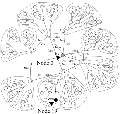
Figure 8: Network simulation topology with 113 nodes
suffer at least the same losses as the ZCRs. However, when ZCRs are not placed at the routing paths, non-nested scopes can have larger recovery delays than non-nested scopes since a receiver gets all the FEC repairs from its own ZCR.
The decision whether a scope is nested within another scope or be a child non-nested scope of another is made when that scope is set up. It should be highly dependent on how the ZCR of that scope is elected. If it is elected manually by designating one receiver at the routing path as a cache, a non-nested scope is more appropriate than a nested one. If the ZCR is elected through a dynamic ZCR challenge, nested scopes may prove more effective as the closest receiver to the sender is not necessarily at the routing path.
5
Simulation
5.1
Simulation setup
We implemented our LMR protocol using the UCB/LBNL/VINT network simulatorns. We incorporated it into three well-known protocols, namely, the basic SRM, a hierarchical SRM, and a tree-based protocol; we compared their performance to that of SRM [1], SHARQFEC [3], and ECSRM [18] respectively. We also implemented our delay estimation protocol, and studied the performance of SRM with this new protocol. Our overall experimental setup is very similar to the one in [3].
Topology. Our simulation experiments were run using variants of the hybrid mesh tree topology used
copy of each other. The links connecting the source to the top 7 nodes in each tree are 45Mbits/s with all other links set to 10 Mbits/s. The latency between any two receivers located within each tree was set to 20 ms for each link while the latencies used for the backbone links are shown in the figures. The loss rates for the links are varied over different parts of the networks.
The loss model. To simulate a realistic loss behavior, we conducted transmission experiments over a
transpacific link every 45 minutes between Oct. 10 and Oct. 13, 1998, and recorded all the packets being received and lost. We gathered over
100
traces each15
minutes long, and extracted the profile information of each trace which comprises the loss characteristics of every non-overlapping 300 ms segment. The loss characteristics include the number of instances of loss bursts of lengths from 1 to over 200. For each link in the networks shown in Figure 8, we find a trace that undergoes the same average loss rate as that of the link, and use the trace to pick packets to drop during each 300 ms period. The loss rates for links are shown in Figure 8. The loss rates that receivers experience can be obtained by compounding the loss rates on the links from the sender to the receivers. In our topologies, they vary from1%
to27
:5%
. Every packet passingthrough a link — data, repair, request, and session — is subject to the same loss rate indicated on that link.
Transmission. Each simulation experiment starts the session at time 1 second, at which time nodes begin
sending session messages, and after the initial bootstrap phase of 6 seconds, node 0 starts sending traffic at a constant bit rate of 800 Kbits/s. Each data packet is 1024 bytes. The sender stops transmitting data packets at time 16 seconds. The block size B is 16, and for all LMR experiments, unless specified, K is set to 5,
and LMR uses the dynamic mode. Note that at this transmission rate, each receiver will get approximately 10 packets over a 100 ms period. In LMR, every receiver determines the required number of FEC packets based on 5% bandwidth wastage threshold as described in Section 3.3.
Parameters of interest. We focus on three categories of traffic: data (this comprises the original data
packets), proactive (this is the traffic transmitted by the sender over and above the data packets without an explicit request from the receivers), and reactive (this is the traffic introduced by the sender or other receivers in response to the retransmission requests). The total redundant proactive (reactive) traffic is the total number of proactive (reactive respectively) packets that reach the receivers in excess of their requirements; total redundant traffic includes both. All ratios and percentages are with respect to the total data traffic received by all the receivers.
5.2
Simulation result
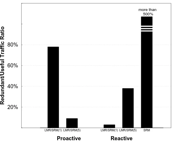
Impact of layering on proactive repair transmission. We measure the impact of LMR in proactive
FEC transmission schemes. We tested single-scoped SRM, LMR/SRM with one repair group (denoted LMR/SRM(1)), and LMR/SRM with five repair groups (denoted LMR/SRM(5)). The result of the simula-tion runs are shown in Figure 9. All transmission tests finished approximately at the same time.
LMR/SRM(1) LMR/SRM(5) LMR/SRM(1) LMR/SRM(5) SRM
20% 40% 60% 80%
Redundant/Useful Traffic Ratio
Proactive Reactive
more than 500%
Figure 9: Impact of layering on proactive repair transmission
3%
redundant reactive repair traffic ratio while that of LMR/SRM(5) is38%
. This is because LMR/SRM(1) aggressively subjects receivers to a large amount of proactive traffic and successfully reduces the chance that further repair packets are needed. However, the total redundant traffic ratio for LMR/SRM(1) is 81% which is 30% more than that for LMR/SRM(5). Thus multi-layering reduces the overall redundant traffic substantially.Comparison of FEC recovery techniques. We now compare the performance of LMR with that of other
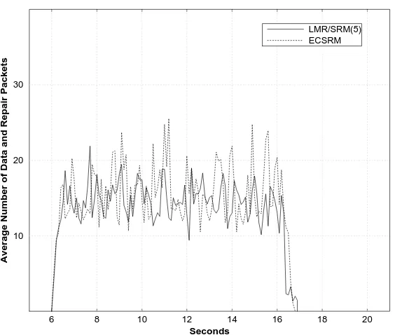
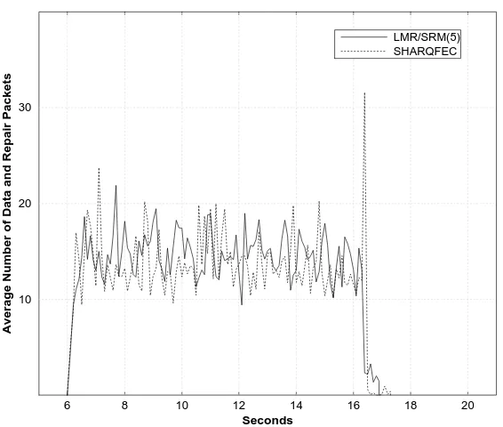
existing FEC recovery schemes. Figures 10, 11, and 12 show this comparison in terms of the average number of packets (of all categories stated above) per receiver received during each 100 ms period. In all simulation tests, the transmission finished at approximately the same time for all the protocols; thus, their throughput is similar. However, they differ in how efficiently they use the bandwidth as described below.
We first compare the performance of LMR/SRM with that of ECSRM [18]. ECSRM is a tree-based protocol that is a version of SHARQFEC where scoping and proactive repair are turned off, and only the sender participates in reactive repair. ¿From Figure 10, one can do a calculation to conclude that ECSRM has about 30% more redundant traffic than LMR/SRM. This is because ECSRM multicasts reactive repair packets, and has poor repair locality. However, the performance of ECSRM is much better than that of the basic SRM we quoted earlier because ECSRM uses reactive FEC repair and also does not allow receivers to participate in the repair. Thus, duplicates in repair transmission are substantially reduced.
6 8 10 12 14 16 18 20 Seconds
10 20 30
Average Number of Data and Repair Packets
LMR/SRM(5) ECSRM
Figure 10: The performance comparison of LMR/SRM, and ECSRM
three-level hierarchy with 29 nesting scopes from the simulation topology in Figure 8 where each bounding circle represents a separate scope, and the roots of 7 trees forms another scope. The root of all the trees in the topology and the sender are ZCRs. SHARQFEC generates only 15% less redundant traffic than LMR/SRM. This result is very encouraging for LMR/SRM because it is only a single scoped protocol while SHARQFEC is extensively scoped. Since SHARQFEC uses 29 scopes of less than five members, the simulation experiment shows excellent repair locality. However, these scopes come with additional cost of maintaining the scopes and ZCRs. This result suggests that LMR can enhance the repair locality of SRM up to the level comparable to that of SHARQFEC.
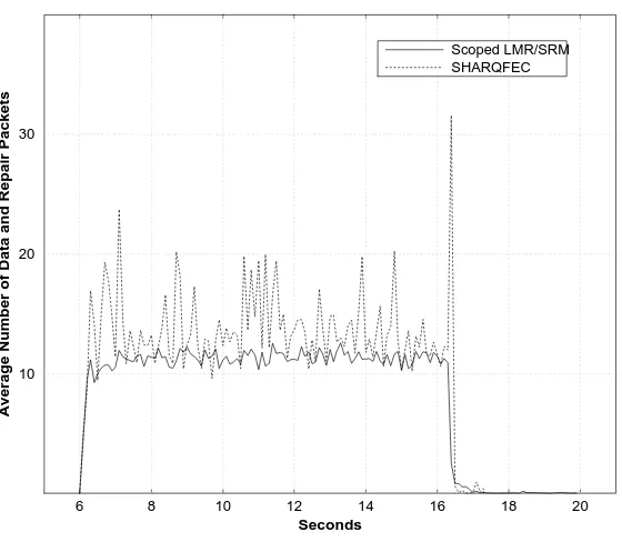
Figure 12 compares the performance of SHARQFEC with scoped LMR/SRM. We allow LMR/SRM to have the same scopes as SHARQFEC in the same topology. The total traffic in scoped LMR is far less than that of SHARQFEC. Overall, scoped LMR has only 19% redundant traffic while SHARQFEC has about 40% redundant traffic. This result strongly suggests that when combined with hierarchical scoping, LMR can achieve excellent repair locality.
Performance of heuristic, optimal and static layering protocols. In this section, we compare the
6 8 10 12 14 16 18 20 Seconds
10 20 30
Average Number of Data and Repair Packets
LMR/SRM(5) SHARQFEC
Figure 11: The performance comparison of LMR/SRM, and SHARQFEC
reactive repair traffic, and thus it is suitable for studying the effect on proactive repair traffic. Figure 13 shows the total number of redundant repair packets received by all receivers during a simulation experi-ment. Recall that the static allocation (i.e., in the static mode) assigns dB=KeFEC repair packets to each
repair group regardless of the current loss rates of receive rs. Under the loss rates assigned to the topology, approximately 8 to 10 repair packets per block are sufficient for the worst case receiver to recover its losses. That is,f
max
10
.The adverse effect of the static allocation is evident when only a small number of repair groups are available. For example, when only one repair group is available, the static protocol multicasts allB repair
packets per block to that repair group while the dynamic protocol multicasts less than 10 repair packets per block. Thus, in the static protocol, many receivers with low loss rates are subject to many redundant repair packets. However, when the number of repair groups gets larger than B=
2
(currently 8), then theperformance advantage of the optimal protocol quickly diminishes, favoring the static protocol because of the overhead of the optimal protocol involved in collecting feedback from all receivers.
6 8 10 12 14 16 18 20 Seconds
10 20 30
Average Number of Data and Repair Packets
Scoped LMR/SRM SHARQFEC
Figure 12: The performance comparison of Scope LMR/SRM and SHARQFEC
6
Related Work
In this section, we review related work in each of the three categories of relevance, namely, multicasting using multiple groups, use of FEC in reliable multicasting, and estimating network delays.
Use of multiple multicast groups. It is a natural idea to consider using multiple multicast groups for
reliable multicasting, and it has appeared before. Previously, it has been applied to congestion control [24, 25, 26, 27] and error recovery [28]. Layering has the potential to work better for loss recovery rather than congestion control because loss recovery does not need any synchronization with other receivers on the common path. The known uses of multiple multicast groups differ from our LMR in the particular layering technique and in their specific applications. In particular, none of the prior work considers the dynamic allocation of repair packets to different multicast groups to optimize repair locality, and do so in a provably optimal manner as we do.
1 2 3 4 5 6 7 8 9 10 11 12 13 14 15 16
Number of Repair Groups
10K 30K 50K 70K 90K
Number of Redundant Repair Packets
Static Heuristic Optimal
Figure 13: The performance comparison of static, heuristic, and optimal allocations of repair packets
sender multicasts different layers of video signals to different multicast groups. Each receiver chooses a subset of multicast groups and controls the amount of its incoming traffic. RLM and LMR are similar since they both allow receivers to adjust the amount of incoming traffic based on receivers’ capability (be it loss rate or its power), but they differ in crucial ways. First, LMR is applied to error recovery whereas RLM is applied to congestion control; also, LMR layers FEC repair packets while RLM layers video data. Hence, the optimization concerns are very different. Second, LMR has a provably optimal way to layer the number of FEC packets while RLM, as it stands, does not have a provably optimal layering strategy. Nevertheless, LMR may be considered as an example of a technique similar to RLM applied successfully to error recovery.
Vicisano et al. [27, 29] also developed a technique to layer bulk data using linear block coding, and ap-plied it to reliable multicast for error recovery and congestion control. The technique is applicable primarily when a large portion of the data is available for encoding prior to transmission. The amount of redundant data in each multicast channel is statically allocated, and it is exponentially spaced amongst channels. Their layering technique replicates data periodically over a fixed time interval, called the window, while keeping every packet within a unique window. Thus, a packet lost in a window can only be recovered from the subsequent windows in the same multicast channel. Therefore, it seems best suited for delay-insensitive ap-plications. In contrast, LMR uses a very different layering technique where the amount of data transmitted to each group is dynamically allocated to minimize the redundant repair traffic. Combined with an ARQ technique, LMR can easily accommodate delay-sensitive applications.