HIGHLIGHTED ARTICLE
INVESTIGATION
Stability and Response of Polygenic Traits to
Stabilizing Selection and Mutation
Harold P. de Vladar1and Nick Barton
Institute of Science and Techology-IST Austria, A-3400 Klosterneuburg, Austria
ABSTRACTWhen polygenic traits are under stabilizing selection, many different combinations of alleles allow close adaptation to the optimum. If alleles have equal effects, all combinations that result in the same deviation from the optimum are equivalent. Furthermore, the genetic variance that is maintained by mutation–selection balance is2m=Sper locus, wheremis the mutation rate and S the strength of stabilizing selection. In reality, alleles vary in their effects, making the fitness landscape asymmetric and complicating analysis of the equilibria. We show that that the resulting genetic variance depends on the fraction of alleles near
fixation, which contribute by2m=S, and on the total mutational effects of alleles that are at intermediate frequency. The interplay between stabilizing selection and mutation leads to a sharp transition: alleles with effects smaller than a threshold value of2pffiffiffiffiffiffiffiffiffim=S
remain polymorphic, whereas those with larger effects arefixed. The genetic load in equilibrium is less than for traits of equal effects, and thefitness equilibria are more similar. Wefind that if the optimum is displaced, alleles with effects close to the threshold value sweepfirst, and their rate of increase is bounded bypffiffiffiffiffiffimS:Long-term response leads in general to well-adapted traits, unlike the case of equal effects that often end up at a suboptimalfitness peak. However, the particular peaks to which the populations converge are extremely sensitive to the initial states and to the speed of the shift of the optimum trait value.
U
NDERSTANDING quantitative genetics in terms ofpop-ulation genetics is crucial for both scientific and practi-cal reasons. However, the development of a consistent theory for long-term evolution has had limited success, because the polygenic basis of quantitative traits makes the prediction of their response to selection immensely intricate, even under the simplest assumptions (e.g., additivity, equal effects of an allele on the trait, and linkage equilibrium) (Barton and Turelli 1989; Keightley and Hill 1990; Turelli and Barton 1994). Most traits seem to be under some form of stabilizing selection, either by the direct action of selection on a trait
whose extreme values are unfit or indirectly by
compromis-ing individual fitness due to pleiotropic detrimental effects
(Keightley and Hill 1990; Mackay 2001, 2010; Hill and Zhang 2012). The joint effects of stabilizing selection and mutation lead to very complicated allele frequency equilib-ria and evolution, and it is not obvious how much genetic
variation they can maintain (Turelli 1984, 1988; Bürger 2000).
An exact analysis in terms of allele frequencies is lacking for polygenic traits with loci of unequal effects. This is desirable, as data from genome-wide association studies (GWAS) yield information about the distribution of single-nucleotide polymorphisms (SNPs) relevant to several traits
based on population sequence data (Hindorff et al.2009;
Visscher et al. 2012). This makes it urgent to understand
how variation at the molecular level explains phenotypic variation. How quantitative variation depends on the num-ber of loci and on the distribution of allelic effects is not clear and is the central question of this article.
Barton (1986) showed that when a population is at equi-librium with the trait mean at the optimum and the alleles
are very close to fixation, then the genetic variance, n, is
2nm/S, where n is the number of contributing loci, m is
the per-locus mutation rate, and Sis the strength of
stabi-lizing selection. In general, the genetic loadLis due to both
deviation from the optimum and genetic variance,L}Dz2+
n, where Dz is the deviation of the trait mean from the
optimum. The contribution of the genetic variance is much
more significant because compared to it, the deviations from
the optimum are very small. Moreover, if the trait is not at Copyright © 2014 by the Genetics Society of America
doi: 10.1534/genetics.113.159111
Manuscript received November 5, 2013; accepted for publication April 2, 2014; published Early Online April 7, 2014.
Supporting information is available online athttp://www.genetics.org/lookup/suppl/ doi:10.1534/genetics.113.159111/-/DC1.
the optimum, higher variance can be maintained. These cal-culations assumed a trait with diallelic loci of equal effects. However, we show that under unequal effects, deviations from the optimum can also maintain less variance.
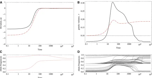
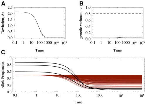
The response to a shift in the optimum trait value will be radically different under equal and unequal effects. For example, Figure 1 shows the response of two equivalent populations that differ only in their distribution of allelic effects. Note that although the traits match the optimum almost perfectly in both cases (Figure 1A), under equal effects much more variation is maintained than under un-equal effects (Figure 1B), which implies a greater mutation load.
We will see that under unequal effects, the equilibria depend on the magnitude of allelic effects. With equal effects, there is a high degree of symmetry in the sense that many allelic combinations match a given optimum value, making it easier to characterize the possible equilibria (Barton 1986). However, this analysis fails under unequal effects because the symmetry is absent. For example, Figure 1, C and D, shows the response of the allele frequencies; in Figure 1, C and D, the alleles have equal and unequal effects, respectively. Initially, the alleles rest at a stable equi-librium that has comparable mean and variance. We see that the response under unequal effects is more heterogeneous in Figure 1D (unequal effects), whereas the alleles respond homogeneously under equal effects (Figure 1C). This differ-ence in the response accounts for the eventual maladapta-tion of traits with loci of equal effects. Moreover, alleles that
have very large effects are at very low frequency and might take substantial time to achieve a higher representation in the population. Thus, anticipating when they will reach in-termediate frequencies and make a notable contribution to the genetic variance is difficult. Also, we do not know which alleles contribute preferentially to the response and even-tual adaptation of the trait. Under equal effects, all alleles have the same contribution, but the symmetry of the solu-tions effectively reduces the genetic degrees of freedom, which in turn limits the possible paths tofind a globalfitness optimum.
The house of cards (HoC) is a mutation–selection balance model that assumes that each allele is new and arises inde-pendently from the previous allele from which it mutated, so that the effects of new mutations are uncorrelated from the previous ones. In equilibrium, the variance of allelic effects is larger than the genetic variance and is predicted to be 2nm/S,
where nis the number of loci, m is the per-locus mutation
rate, and Sis the strength of stabilizing selection (Kingman
1978; Turelli 1984; Bürger 2000, Chap. IV). Exactly this amount of genetic variance is maintained for traits with sev-eral diallelic loci of equal effects, when they are adapted to the optimum (Barton 1986). However, numerical experi-ments such as the one shown in Figure 1B reveal that with unequal effects, the genetic variance is decreased even farther below this bound. It is not immediately clear why this differ-ence between traits with equal and unequal effects occurs.
Although the HoC assumes a continuous production of new alleles with varying effects (Turelli 1984), this model
can be interpreted as a limit of a trait consisting of many loci
(Barton 1986), in which case each locus composing a traitz
under stabilizing selection evolves according (as is explained in detail below) to
dp
dt¼ 2Sgpð12pÞð2Dzþgð122pÞÞ þmð122pÞ; (1)
where p is the frequency of the “+” allele, g is its allelic
effect, and Dz is the deviation of the trait mean from the
optimum. Detailed analyses of this system under equal effects were performed by Barton (1986). At equilibrium, the equation above can have one or three solutions for each
locus, given by the cubic polynomial onp that results from
equating dp=dt¼0: If we plot the equilibrium value of p
against Dz/g, we find that there are two types of curves,
depending on the mutation rate, m (Figure 2A). The first
type (Figure 2A, thin curve) occurs at high mutation rates; in this case and at small deviations from the trait optimum, the equilibrium is maintained at intermediate frequencies, maintaining substantial variability. The other type of equi-librium (Figure 2A, thick curve) occurs when mutation rates are low compared to the mutational effects: for well-adapted traits either of the two alleles can be nearfixation, each one
contributing to the genetic variance by 2m/S, as the HoC
predicts.
Under equal effects the equilibrium value of the trait
depends only on the number of + and “2” alleles, thus
allowing many equivalent genetic combinations; there are many other stable but suboptimal combinations (Barton 1986). The particular state to which the population con-verges is thus strongly determined by its previous history. All these suboptimal combinations trap the population in
localfitness peaks that deviate considerably from the
opti-mum trait value. We can see in Figure 2A (thick line) that if the effect of each locus on the trait is fairly large, then deviations from the trait that are at most equally large as
the effect can maintain any + or 2alleles at equilibrium.
Thus, many of the suboptimal combinations are realizable. Also, if the population is resting at an initial equilibrium and the optimum is shifted (either slowly or abruptly), the allele frequencies respond in a coordinated way. Thus, the trait is resilient to perturbations in the sense that all allele frequen-cies are always equidistant from the bifurcation point where their stability changes and thus resist large deviations from the optimum. Once the bifurcation point is reached, all loci become unstable at once and suddenly jump to a suboptimal state. Therefore, it is unlikely that populations reach an optimal peak.
In this article we show that if the loci that constitute the trait have different effects, there is a more heterogeneous distribution of equilibria, with no symmetry among peaks. There are still many suboptimal states where the population could get stuck, but we will see that under unequal effects, these suboptimal equilibria are much more similar (and closer) to the optimum. However, the trait is also less resilient to deviations from the optimum, and smaller perturbations
render the configurations unstable. In fact, we see in Figure
2A that alleles of very small effects will make Dz/g large,
implying that the allelic configurations become unstable. Nat-urally, the occurrence of small effects is contingent on the distribution of allelic effects, which is unknown in detail; we explore this aspect in this article.
Summarizing, under equal effects precise adaptation to the optimum is harder because the population might get stuck at suboptimal peaks that have large variation and larger mutation load. At equilibrium, selection purges the new mutations and irrespective of their allelic effects, each locus contributes 2m/Sto the genetic variance. In fact, this is an upper bound achieved when the trait is perfectly adapted to the optimum, irrespective of the distribution of genetic effects (as long as these are larger than their contribution to
Figure 2 (A) Equilibria of allele frequencies as a function of scaled de-viation from the optimum. Thin curve shows equilibria for alleles of small effects (g2, 4m/S); for each value of Dz/g there is one stable allele
frequency. Thick curve shows equilibria for alleles of large effects, (g2.4m/S); for small deviations from the optimum, there are two possible
equilibria nearfixation. The dashed segments are unstable equilibria. (B) Equilibria of allele frequencies as a function of the scaled parameter
m=m/g2S. Thick shaded curve shows no deviations from the optimum,
the genetic variance in equilibrium). However, if the trait mean deviates from the optimum, the genetic variance can differ from that of the HoC (Bürger and Hofbauer 1994) (Figure 1).
A different situation is realized if the allelic effects are smaller than the equilibrium variance, for which the HoC model does not apply. Another classic approximation, which supposes multiple alleles and is often referred as the Gaussian model (GM) (Kimura 1965; Lande 1976), makes
the opposite assumption about the allelic effects, i.e., that
these are small compared to their contribution to the genetic variance in equilibrium. The GM assumes that there is a con-tinuous production of new alleles that follows a Gaussian distribution of effects at each locus that is centered at the parental genotypic value. Barton (1986) showed that in polygenic diallelic traits under equal effects, changes in the optimum can lead the population toward stable albeit maladapted equilibria that can have much larger variation than that of the HoC and fall into a limit that is better approximated by the GM.
The analyses for polygenic systems with unequal effects that we perform here are more challenging than for equal effects. Our current understanding of unequal effects derives from models that deal with a few loci, from which general results are hard to extrapolate (Turelli 1984; Bürger 2000;
Chevin and Hospital 2008; Pavlidis et al.2012). In this
ar-ticle we aim to understand how a trait determined by arbi-trarily many loci of unequal effects responds to stabilizing selection and mutation. Putting aside the technical complex-ities, we regard this problem as fundamental to understand-ing the bigger picture of the evolution of polygenic traits,
namely that of finite populations subject to drift and how
these are constrained by pleiotropic effects caused by
selec-tion on multiple characters. Butfirst, we need to understand
in detail the nature of the equilibria and the response of allele frequencies to factors such as stabilizing selection and mutation. Thus, we address the simplest case of deter-ministic selection on a single trait.
We start by studying the equilibria andfind that there can be multiple loci with high polymorphism, provided that they have small effects. For these alleles of small effect, devia-tions from the optimum trait value are tolerated without
affecting their equilibrium. However, we alsofind that there
is a threshold g^¼2pffiffiffiffiffiffiffiffiffim=S that objectively defines which alleles are of “small” effectðg,g^Þ and which ones are of “large” effect ðg.^gÞ: The former remain at intermediate
frequencies and the latter near fixation most of the time.
Alleles of large effect can be sensitive even to small devia-tions from the optimum. In particular, if the optimum is
suddenly shifted, wefind that the alleles that respondfirst
are those with effects closer to the threshold value,gg^:In the long term, however, the dynamics are intricate. Different initial equilibrium configurations that are equally well adapted may lead the population to totally different regions of the
fitness landscape. However, these different genetic states
have very similar phenotypic values.
Model of Stabilizing Selection and Mutation on Additive Traits
We consider the simplest diploid genotype–phenotype map,
which assumes an additive trait for diallelic loci, without dominance or epistasis,
z¼X
n
i¼1
gi
XiþXi921
; (2)
wheregiis the allelic effect at locusi,nis the number of loci
composing the trait, and X and X9are indicators of the 2
allele (X,X9= 0) or of the + allele (X,X9= 1). We allow
each gi to vary across loci. Specific values are drawn from
a given distribution (we explore mainly gamma distributed effects), although in every run they are kept constant. As-suming linkage equilibrium, the trait mean and the genetic variance are given by
z¼X
n
i¼1
gið2pi21Þ (3)
n¼2X n
i¼1
g2ipið12piÞ; (4)
wherepi=e[Xi], the allele frequency of the + allele, given
by the expectation ofXiin the population. (Unless otherwise
stated, the expectations are on the population, not on the distribution of effects.)
We assume a Gaussianfitness,Wz¼exp½2ðS=2Þðz2z∘Þ2
so the meanfitness of the population is
W¼exp
2S 2Dz
22S
2n
; (5)
which assumes weak selection. The genetic load is due to
both terms: the deviations from the optimum Dz¼z2z∘
and the genetic variance n. The maximum meanfitness is
1, which occurs if an optimal genotype is fixed, with no
genetic variance.
In an infinite, random-mating population, the change in
allele frequencies is given by the selection–mutation
equation
dpi
dt ¼ 2Sgipið12piÞð2Dzþgið122piÞÞ þmð122piÞ;
(6)
for i = 1,. . .,n, and m, S 1 (see, for example, Barton 1986). This equation for the dynamics of allele frequencies assumes linkage equilibrium and weak selection.
To understand the complexities of the fitness landscape
wefirst study the qualitative aspects of the equilibria of
Equa-tion 6, by assuming that Dz is given, which uncouples the
equations. This gives a solid intuition to understand detailed equilibrium analyses and how much genetic variance can be maintained at the different suboptimal peaks.
Afterward, we explore the dynamics and understand the irregular behaviors by using the intuition derived from the equilibrium analyses. We numerically solve the system for all the allele frequencies at each locus. Since we assume diallelic loci, there arenequations to track. We calculate the
genetic variance and trait means from the definitions given
by Equations 3 and 4. We typically randomize the initial conditions and the realization of allelic effects, unless other-wise stated.
Allelic Equilibria Have Two Defined Regimes
Equation 6 shows that the equilibrium condition for every locus is given by a set of cubic equations coupled through
Dz. When there are many loci, we can assume a particular
value forDzand treat each of thenequations independently. Therefore, for each locus the number of valid roots of the cubic equation depends on four quantities: the deviation from the optimumDz, the allelic effectgof the focal locus, the mutation ratem, and the strength of stabilizing selection S. However, these four variables can be combined into just
two scaled parameters, d=Dz/gandm=m/Sg2, and the
equilibrium solution at each locus is given by the scaled equation
p32p2
3
2þd
þp
1
2þdþm
2m
2 ¼0: (7)
Figure 2A shows how the equilibrium frequencies depend on
the scaled deviation from the optimum,d. These diagrams
also hold for unequal effects, except that the equilibria for
each locus are represented by a specific diagram. In
Appen-dix Awe give the precise expression of the critical points of
Equation 7. Figure 2A shows that there may be two types of equilibria: either nearfixation of one or the other allele or a single equilibrium at intermediate frequency 1/2. The fac-tor that determines which equilibrium is attained at a given locus is the scaled variablem=m/Sg2.
Figure 2B shows the equilibrium allele frequencies as
a function of m. Considerd = 0: we see a partitioning of
two qualitative regions with stable states that are nearfi
xa-tion (m , 1/4, to the left) and intermediate equilibrium
(m.1/4, to the right). Note that sincemis inversely propor-tional tog2, the smaller the effects are, the more to the right
the alleles are represented in Figure 2B, and vice versa. Thus ^
g¼2pffiffiffiffiffiffiffiffiffim=Sis a threshold that objectively defines alleles of large and small effect: ifg.g^;these fall into the category of large effects, and ifg,g^;these fall into the category of small effects.
Figure 2B shows how this diagram is modified ford6¼0:
the bifurcation is shifted, and the intermediate equilibria
close tom$1/4 are displaced from 1/2. This has two main
implications. First, assume a small deviation ofd.0 (d,
0); some of the alleles of large effect that would have been close tofixation, at the + (2) state, are forced to sweep to the alternative state. Second, some of the alleles of small
effect that would be at the intermediate state,P= 1/2, will
show reduced (increased) frequencies. Most notably, the alleles that are displaced are those that are close to
m¼m^; which are those that are close to the threshold
^
g¼2pffiffiffiffiffiffiffiffiffim=S:
A bigger picture emerges when we consider how the
equilibria depend on combinations of both d and m (see
Appendix A for the exact calculations), which is shown in
Figure 3. On a logarithmic scale, the allelic effects fall on a straight line, with the distribution of effects determining their spread along this line: smaller effects fall toward the right and larger effects fall toward the left of the diagram; different values ofdare represented as parallel lines of slope 1/2.
When effects are large enough that m,m^ ¼1=4; the
alleles can be in a bistable regime: there are two stable
points close to fixation and one unstable at intermediate
frequency (the thick line in Figure 2A). This is provided that
deviations from the optimum are small (d0). In this case,
the stability is not affected. However (and as we explain
below), deviations that are of the order$d1/2 disturb this
equilibrium (see Figure 2B).
The situation is very different for small effects, whenm. 1/4, since there is only one valid root of the cubic above (the thin line in Figure 2A). When the trait is close to the
opti-mum (d0), intermediate frequencies can be maintained,
as explained above. Small deviations from the optimum will readjust frequencies slightly, but the stability of the
equilib-rium is not modified (there is no qualitative change in the
stability).
As a consequence, the frequency of alleles of small effect varies smoothly with the deviations from the optimum, whereas those with larger effect experience discontinuous transitions when the magnitude of the deviation approaches half of their respective effects.
The scaling properties indicate that the parameters that really matter arem=m/g2Sandd=Dz/g. Thus, the
spe-cific numerical choices of m and S are not in themselves
decisive.
Stability and Variation at Equilibrium
Equilibria under mutation–selection balance
As above, when mutation is present, there might be one or three solutions for each locus, with the stability depending on the particular multidimensional adaptive peak. Conse-quently, there might be up to 3npossible equilibria, although
only a fraction of these can be stable. Assuming equal effects, it would be enough to count the number of loci that
are fixed or intermediate, since the symmetry of the
these peaks (Barton 1986). With unequal effects, we need to
consider each of these configurations separately. These are
tractable as long as we assume thatDz= 0, in which case
the equilibria at each locus are given by
0¼ m2Sg2pð12pÞð122pÞ: (8)
In this case there are three possible states for each locus, namely
p¼1=2 (9)
p¼1
2
16
ffiffiffiffiffiffiffiffiffiffiffiffiffiffiffiffiffiffiffiffi
124 m
Sg2
r
: (10)
InSupporting Information,File S1we detail the stability analyses that we now summarize. In the absence of muta-tion, at most one allele can be maintained polymorphic, irrespective of the magnitudes of the allelic effects and of the deviation from the optimum (this result was anticipated by Wright 1935). If mutation rates are small compared to selection, the trait mean is exactly at the optimum, and all alleles are of large effects, then the configurations where all loci are close to fixation will be stable (all eigenvalues are
negative). Furthermore, configurations where alleles of
large effect are at intermediate frequency will be unstable. We alsofind that configurations where alleles of small effect
are near fixation are unstable.
Why is this? Alleles with large effects increase the genetic
variance substantially. We saw that each allele nearfixation
contributes 2m/S, whereas if it has intermediate frequency, it
contributes g2/2 to the load. Since the alleles with large
effects fulfill thatg2/2.2m/S, the genetic load would be
much larger if the alleles of large effect were maintained polymorphic. A similar argument applies for alleles of small effect. Becauseg2/2,2m/S, then the load would be
signif-icantly higher if these alleles were near fixation. We can
interpret this by thinking that the amount of selection re-quired tofix alleles of small effect would need to be consid-erably high, to make them fall into a“large effect”class.
Distribution of allelic equilibria
We saw that alleles of large effect will be in near fixation.
However, whether they are more likely to be at the + or
the 2 state depends on details such as the position of the
optimum and the deviation from it. For example, in File S2
we show that optima positioned toward the largest (smallest) trait valuezxbias alleles to the + (2) states. Can we estimate
how likely are alleles to be close to a particular state? We assume that the trait mean is at the optimum and focus on the state of one particular allele. We study how the probabilityrthat the focal allele is at the + state depends on its effectg. In this case, we takerto be a probability calcu-lated over all possible states (peaks), where we assume that the rest of the (background) loci contribute in a way that keeps the trait at the optimum. We assume that for all alleles of large effects the initial conditions are such that Pr0(2) =
Pr0(+) = 1/2. Numerically, we perform many runs that start
close to uniformly randomly selected peaks and let the sys-tem reach equilibrium. Then we count how often alleles of
effectgare in the + state. InAppendix BandAppendix Cwe
show that
rj¼ 1
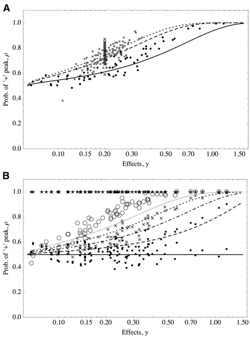
1þexph22ðz∘=VÞqgffiffiffiffiffiffiffiffiffiffiffiffiffiffiffiffiffiffiffiffiffiffiffiffiffiffi2j 24ðm=SÞi; (11) where V ¼P9i6¼jðg2i 24m=SÞ; where P9 indicates summa-tion on the set of alleles of large effect. Figure 4 shows that the predictions of Equation 11 are consistent with the sim-ulations. The distribution of effects does not affect the prob-ability of an allele being in the + or2state; only the effect of the focal allele matters.
The larger the effect of the focal allele is, the larger the probability it is in the + state (this assumes positive positioning of the optimum; for negative positioning, the converse would be true). The reason is that alleles that are closer to the threshold value are more prone to the instabilities
resulting from small deterministic fluctuations around the
optimum. Large alleles, on the other hand, are more often at the + state since they are more resilient to perturbations from the optimum value. Thus, once a population attains
equilibrium, large alleles with effects close to ^g are much
more likely to be stuck in alternative equilibria than larger alleles.
We alsofind in Figure 4B that the larger the value ofzois,
the larger the probability for all loci to be in the + peak. This
is expected, because lager trait values require more + alleles. This obvious observation, although supported by the model, is quantitatively underestimated by it. In princi-ple, deviations from the optimum trait value can be accom-modated in Equation 11 (Appendix C). But this correction, at
least to first order on Dz, does not fully account for the
underestimation of the model at large optimum values (data not shown). What actually happens is that as the optimum is positioned closer to the range of response of the trait, the distribution of traits is considerably skewed and the Gauss-ian assumption fails.
Above we saw that alleles with effects that are close to the critical point are more susceptible to small perturbations
to the optimum. Thus how stable the trait is to small shifts of the optimum depends on how far the frequencies are from the critical point, which in turn depends on the particular distribution of allelic effects. Under equal effects, all alleles are equally far from the critical point and thus remain stable for a long period until the deviation is large enough. But when the deviation reaches the critical value, all alleles are perturbed at the same instant.
Under unequal effects the picture is more complex. The individual equilibria of each allele are perturbed differently by deviations from the optimum. Moreover, once a given allele is perturbed and placed at an alternative state, the newly attained equilibrium is characterized by a different deviation from the optimum, potentially perturbing yet another allele. The interplay among the complex equilibria is hard to characterize in detail.
Now we determine the size of the deviations from the optimum. By employing perturbation analysis (Appendix B)
we find that positive deviations from the optimum push
allele frequencies closer tofixation. We also prove that the
maximum deviation close to a given peak is of the order ~
Dz’mini2Lgi=2;whereLis the set of large effects (in
Ap-pendix Bwe give an exact expression to the maximum
de-viation). Clearly, this is bounded below by ︹g=2; and D~z depends on the particular draw of effects. This limit for the deviation is suggested by the diagram in Figure 2A: we see that the shoulders of the black lines actually occur relatively neard= 1/2 (as long as effects are large enough). Consequently, we expect that most of the time the traits will be fairly well adapted, and most of the load is given by the genetic variance, rather than by large deviations of the mean from the optimum.
Genetic variance
By direct substitution of Equations 9 and 10 into Equation 4 we see that the genetic variance that is maintained by mutation–selection balance isg2/2 per locus at the
interme-diate state and 2m/Sper locus nearfixation. Contrast this to the genetic variance predicted by the HoC, which is the same as for traits controlled by equal but large effects; i.e.,
n = 2nm/S. Under unequal effects, ifDz = 0, the genetic
variance is
n¼2nf
m
Sþ
1 2
X
k2S
g2k; (12)
wherenfis the number of alleles of large effect, and the set L contains the ns alleles with small effects, g2/2, 2m/S;
clearly,n=nf+ns. Note that thefirst term is due to alleles
that are close to fixation, and their contribution to the
ge-netic variance is independent of their effect, and the second term is due to alleles of small effect, which are at interme-diate frequency. Equation 12 is one of our central results.
With this result we come back to Figure 1: in Figure 1B the genetic variance of the trait with unequal effects is lower than that of the HoC. That is because 24 alleles are of small effect.
Figure 4 The probability of + alleles increases as the magnitude of their effect gets larger. Lines follow Equation 11; symbols show average of occurrences of the + state from 100 simulations. (A) The optimum isfixed and the distribution of allelic effects is varied.zo= 10 (roughly halfway
from the maximum trait value). Solid line and solid circles show exponen-tial distribution (mean = 1/5); dashed line and shaded squares show gamma distribution (shape = 20, scale = 1/100); dotted line and crosses show equal effects,g= 1/5. (B) The distribution of allelic effects isfixed and the position of the optimum is varied. Effects are distributed as an exponential (mean = 1/5); thick solid line and solid circles showzo= 0,
dashed line and solid squares showzo= 5, dotted-dashed line and crosses
showzo= 10, dotted line and open circles showzo= 15, and thin solid
line and stars showzo= 20. In all cases the trait is determined by 100 loci. m= 1024,S= 0.1. The initial conditions were uniformly and
Equation 12 correctly predicts the equilibrium variance,n=
0.064. However, note that if we use the HoC withnf(instead
ofn), thenn’0.052,.80% of the total variance.
Thus, the HoC variance bounds the genetic variance under unequal effects. Specifically, Equation 12 implies that
nHoC(nf)#n#nHoc(n), wherenHoC(m) is the HoC variance
withmloci. With no deviations from the optimum, the load
is proportional to the genetic variance. Under the HoC the
load is always L = Sn/2 = nm. However, because under
unequal effects the genetic variance is smaller, the muta-tional load will also be smaller and dependent on the distri-bution of alleles.
The equilibrium genetic variance depends on the distribu-tionP(g) of allelic effects. Even though alleles nearfixation contribute tonindependently ofg, the proportion of alleles of
large effects will change with P. For example, fixing the
expected value of g at a value larger than ^g; but allowing
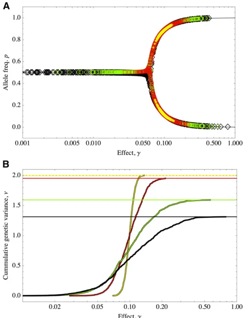
the shape of the distribution to change, will result in different proportions P=nf/nof alleles of large effect (Figure 5). In
this way, we keep the whole range of response of the trait comparable across different distributions of effects. Distribu-tions peaked around the mean will correspond to traits with alleles of large effect, all of which will be nearfixation (Figure 5A, yellow stars); thus 100% of the variance is due to alleles of large effects and will match the HoC variance (Figure 5B, yellow curve). For distributions that are more spread, the traits will have mixed effects (Figure 5, red squares/line
and green circles/line):ns increases to 96, with7% of the
variance due to alleles of small effects, andns= 342,17%
of the variance is due to alleles of small effects (red and green, respectively). The extreme case will be for positively skewed distributions, such as the exponential, where the pro-portion of alleles of large effects is much smaller (Figure 5A, black diamonds), and the genetic variance will be consider-ably lower than that of the the HoC (Figure 5B, black curve): roughly half of the alleles (ns= 478) are of small effect, but
contribute by 20% to the total variance.
Distribution of phenotypic equilibria
For many loci, the number of allelic equilibria can be astro-nomical. Nevertheless, under equal effects it can be calcu-lated explicitly (Barton 1986). When mapped to trait mean and genetic variance, the number of distinct equilibria is smaller, since many combinations of allelic effects have equivalent, or at least very similar, trait mean and variance. Figure 6 shows how the phenotypic states change when we keep the mean of the allelic effects constant, but increase its variance: the genetic variance decreases (see also Figure 5), and deviations from the optimum have less effect on the genetic variance, making Equation 12 a good
approxima-tion. Notably, we find that the number of values of trait
mean and genetic variance increase when the distribution of effects spreads. However, these equilibria become more similar and closer to each other.
Although it is hard to count the states precisely, we can study how a given phenotypic equilibrium is affected as the
asymmetry of the unequal effects is increased. For instance, suppose under equal effects we track a set of initial
conditions Pthat lead to a particular point in the “
pheno-typic” ðz;nÞ-space. The states to which these trajectories converge (basins of attraction) are symmetric in the sense
that exchanging + alleles at one locus with 2 alleles at
another does not change the phenotypic states. If we keep
constant the set P, but now change one effect by a small
amount, how is the distribution of phenotypic states
af-fected? Many of the trajectories starting at P that under
equal effects converged to equilibria characterized by the same trait mean and variance will now converge to different
points in ðz;nÞ-space. The symmetries are broken and
ex-changing alleles at that locus with another one affects the trait mean and variance. Hence, the phenotypic equilibria show bifurcations when we perturb the effects. We can
Figure 5 (A) Equilibria under different distributions of allelic effects. Sym-bols show data from simulations. Initial frequencies were drawn uniformly in (0, 1) and the system numerically evolved to equilibrium. Gray lines show equilibria of allele frequency and symbols show numerical equilib-ria. (B) Cumulative contribution to the genetic variance under different distributions of allelic effectsP(g). Solid curves show data corresponding to the simulations in A. Solid horizontal lines show equilibrium genetic variance (Equation 12). Dotted line shows genetic variance of the HoC.
P(g) is a gamma distribution of mean = 0.1 with shape parameterspas follows: yellow, stars,p= 1023; red, squares,p= 1022; green, circles, p= 531022; and black, diamonds,p= 1021.m= 1024,S= 0.1,n=
repeat this procedure by then perturbing a second locus, and so on. Thus, if we represent the phenotypic states as nodes, and we connect these nodes according to the initial condi-tion that led to their corresponding phenotypic states, we will have a graph that represents the increase in complexity of the adaptive peaks. Unless we have a way to cover the initial space uniformly, this does not ensure complete count-ing of the number of phenotypic equilibria. However, even if the subsampling of the basins of attraction is poor, the
method quantifies how complex the space becomes as we
increase the variance of the allelic effects.
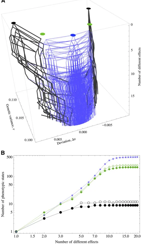
If we carry out this procedure for different phenotypic states under equal effects, then we will have several of these graphs. If these graphs share nodes, then it means that the adaptive landscape is more accessible to better-adapted equilibria (because under unequal effects the equilibria have less genetic load, Figure 6). In fact, in Figure 7 we see an example for three graphs derived from the optimal peak and two suboptimal peaks.
Altogether, this exposes that under unequal effects the fitness landscape is more complex or“rough”, but the solu-tions are generally closer to the optimum. Surprisingly, per-turbing slightly the effect of only one or two loci is enough to overlap different graphs with common nodes, indicating that unequal effects act like a funnel to guide the trajectories to nearly optimal states.
Initial Response to Selection
We saw that there are two well-defined regimes that clearly
separate alleles of large effect from alleles of small effect. If
the optimum shifts, which alleles respond first? A related
question is, Is the initial rate of change of the trait driven mainly by alleles of large or small effect? Although these
two questions are related, they are not the same; even if, for
example, alleles of small effect sweep first, they might not
drive a substantial displacement of the trait. Conversely, even if an allele of large effect sweepsfirst, its overall effect might be negligible when compared to a background of very many loci of small effect.
To calculate the rate of response of an allele, assume that the population is at equilibrium at a local peak with no
deviation from the optimum that is at zo. Suddenly, the
optimum is placed at another value zf. Equation 6 implies
that at each locus
Figure 6 Phenotypic equilibria under different distributions of effects. Shaded circles, equal effects; small solid circles, effects tightly clustered around the mean (gamma distributed with variance = 1/1000); crosses, exponentially distributed effects (variance = 1/100). In all cases the mean effect is 0.1. Points are results from numerical calculations for 11 equi-distant optimazo2 ½2zx=2;zx=2;zx¼g¼5;at each point employing 200 runs with uniform random initial conditions.m= 1024,S= 0.1,
n= 50.
Figure 7 (A) Connectedness of macroscopicfitness peaks as the number of different effects of a polygenic trait is systematically increased from 1 to 20. The thick black lines originate at suboptimal equilibria, and the thin blue lines originate at the optimal equilibrium (dz= 0). (B) Number of new equilibria derived from the suboptimal equilibria under equal effects (black circles and green diamonds) and at the optimum equilibria (blue stars) as the number of different effects is increased.m= 1024,S= 0.1,
dp
dt ¼2SgpqDV; (13)
where DV=zf 2 zo. For alleles of small effect, the
right-hand side isðSg=2ÞDV:Therefore, alleles with infinitesimally small effects will be nearly neutral and will have a vanishingly small rate of response to selection. As the effects become closer to (but still smaller than) g^; the rate of response is larger. Consider now alleles that have infinitely large effects. The right-hand side of Equation 13 isð2m=gÞDVand implies that since these alleles will be almost fixed, there is little variation to select on. Consequently, their rate of response is also vanishingly small. As the effect become closer to (but still larger than) ^g;the rate of response become larger. Therefore, those alleles with effects close to ^gwill have the earliest response to selection because they are the most sen-sitive to deviations from the optimum. Thus, the maximum response for each limit is given by the effect that is exactly at the critical value^g:Evaluating Equation 13 at^gwefind that the rate of response is at most
dp dt
max
¼pffiffiffiffiffiffimSDV; (14)
indicating that alleles with effects close to^gdrive the initial response of the trait to selection.
Long-Term Response to Selection
The long-term response of a polygenic character to the displacement of the optimum trait value can be driven by alleles other than those of intermediate effect. Although the alleles of large effect evolve slowly in the beginning, they can eventually gain representation and evolve much faster. A general closed solution for the dynamics is neither possible nor useful, as the behavior of the allele frequencies is rather complicated. The question is whether the theory developed above can be useful to gain insight into the long-term response of the trait.
Abrupt displacement of the optimum
We assume that repositioning the optimum happens always within the range of response of the trait and far from the
extreme values given byzx¼
P
gi;i.e.,2zxzozx. The
equilibrium analyses revealed that the particular position of the optimum is not decisive for equilibria or stability. Instead the deviation from the optimum is the important factor. Thus, if the population eventually adapts to the new opti-mum value, the genetic variance that is maintained at the newly established equilibrium will be more or less the same as in the beginning. In the transient time, the dynamics will
be complicated and depend on the specific initial conditions
(the adaptive peaks where the population initially stands) and on the distance to the optimum.
If the optimum changes abruptly and is larger in magni-tude than the largest of the effects, all the equilibria will be
perturbed, favoring an increase in the frequency of the those alleles that diminish the deviation from the optimum. That is, if the new optimum value is smaller (larger) than that of the
original optimum value, 2 (+) alleles will increase in
fre-quency. This displacement is seen in the diagram in Figure 3 toward the top (where only one stable border is initially beneficial), with a gradual return of the line to low values of
Dz. Therefore, we expect to observe a transient increase in
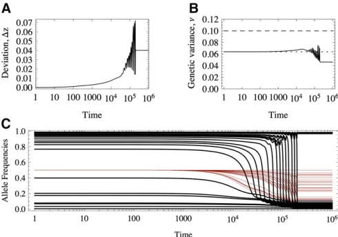
the genetic variance. Figure 8 provides an example where these patterns are in fact found.
In the example in Figure 8, of 50 loci, 26 are of large
effect and contribute.80% of the initial variance, whereas
24 are of small effect, contributing the remaining 20% of the variation. In Figure 8C we see that many of the large alleles shift in frequency and some sweep, transiently raising the genetic variance. In this case, since the optimum shifts from zo= 2 tozo=22, the + (2) alleles decrease (increase) in
frequency. Alleles of small effect are displaced, but not sub-stantially. Most of the transient variation that is generated is due to sweeps of alleles of large effects.
As hypothesized above, even if transient dynamics are very complex (Figure 8), when a new equilibrium is attained,
the final deviations from the optimum are small, and the
genetic variance is close to that of Equation 12 (see also Figure 1). As we saw in the Introduction, under equal effects the population will evolve to a suboptimal state where plenty of genetic variation is maintained. Why do populations end up better adapted under unequal effects?
At first we might think that a bulk of alleles of small
effects could provide enough background variation, allow-ing the population to explore the genetic space more efficiently. However, the response of a trait constituted only
Figure 8 Response to an abrupt displacement of the optimum of a poly-genic trait. (A) Deviation of the trait mean from the newly positioned optimum. (B) Genetic variance. Solid black line, exact numerical results; dashed black line, house of cards prediction (n= 2nm/S); dotted black line, exact value from Equation 12. (C) Response of the allele frequencies: black lines, alleles of large effect; thin red lines, alleles of small effect. The trait is constituted by n= 50 loci, 26 of large effects and 24 of small effects, distributed as an exponential of mean = 1/10. m= 1024, S=
by alleles of large effect is virtually the same as that of a trait that contains also alleles of small effect, in as much as the initial genetic variation contributed by the latter alleles is small, and the optimum is not too close to the maximum trait value (File S3). Thus, concerning the response, alleles of small effect can be regarded as nearly neutral.
Another plausible explanation lies in the rate of“benefi
-cial mutations”(in the sense that these are mutations that
approach the trait mean to the new optimum). Because un-der equal effects the response of allele frequencies is
syn-chronized, most mutations are initially beneficial. However,
due to the epistatic nature of the fitness landscape, those
initially beneficial mutations are not necessarily beneficial once the rarer alleles have increased their representation in the population and might even become detrimental. Fur-thermore, these alleles arise and increase their frequency on the same timescale. Under unequal effects different mutations arise at different times and can compensate the load contributed by previous mutations. In fact, because of
epistasis, we expect and in fact we find (Figure 8C) that
some alleles that are initially beneficial increase in
fre-quency, but afterward become detrimental and decrease in
frequency again. This“prevention of sweeps”has been
ob-served in polygenic traits with up to eight loci (Pavlidiset al. 2012). However, under equal effects allele frequencies re-main synchronized along evolution, and it is unlikely that the initial conditions and the shift in the optimum are in
generalfinely tuned in such a way to allow the population
to reach a local peak that is close to the global optimum. Since the previous examples suggest that adaptation is driven mostly by alleles of large effect, an interesting question that follows is, What happens when traits are controlled principally by alleles of small effect? First of all, Equation 12 indicates that the genetic variance will be much lower than
that of the HoC. We find that the population eventually
adapts (although somewhat slower), but with virtually no change in the genetic variance. In this example, the trait has only three alleles of large effect, which contribute 11% of the genetic variance, and 397 loci with alleles of small effect, which contribute the remaining 89% of the variation. The three alleles of large effect sweep, but ultimately do not affect the genetic variation substantially (assuming their HoC contribution), and some alleles of small effect are strongly shifted.
Figure 9 shows the response of a system of alleles of prin-cipally small effects. Although 400 loci determine the trait, we estimate that the effective number of allelesne’28 (see
File S4). Assuming constant genetic variance given by the HoC (but usingne), wefind that directional selection toward
the optimum explains the response of the trait (although it
fails to predict a minor final deviation from the optimum).
This experiment highlights why we might find stasis of the
genetic variance and a sustained response to selection, which is caused by innumerable alleles of small effect. Under these circumstances, although experimental assays would be able to detect only a few major loci (Hindorffet al.2009; Visscher
et al.2012), these turn out to be the least relevant to explain
the quantitative genetic variation.
Slowly moving optimum
If the optimum is shifted slowly enough, the deviation Dz
remains very small. We also see that the genetic variance then hardly changes (for example, Figure 10). After some time the population keeps evolving but reaches a stationary state. If the optimum suddenly stops, the population settles at a state characterized by a lower genetic variance, but larger deviation from the optimum as in the case when it adapts to a rapid shift of the optimum, as in the previous section. How can we explain these patterns?
Under the infinitesimal model the population achieves
a stationary lag from the optimum given byDz*=2k/2Sn,
where kis the speed of the moving optimum (Lynch and
Lande 1993; Joneset al.2004). However, we see in Figure
11 that this approximation fails for afinite number of loci of unequal effects.
Suppose that a moving optimum changes linearly in time:
zo(t) := V0 + (Vf 2 V0)t/T. For simplicity we consider
optima starting at 2V and ending atV. Hence the speed
of the moving optimum isk= 2DV/T.
By summing Equation 6 over loci and using Equations 3
and 4, wefind that during transient evolution the deviation
from the optimum is given by
dDz
dt ¼ 22nDzþSm322mz2k; (15)
Figure 9 Response to an abrupt displacement of the optimum of a poly-genic trait constituted mainly by alleles of small effect. (A) Deviation of the trait mean from the newly positioned optimum. Solid black line, exact numerical results; dashed gray line, approximation assuming an effective number of loci,neff= 28 and constant genetic variance,n’
2nem/S(see text). (B) Genetic variance. Solid black line, exact numerical
results; dashed black line, house of cards prediction, (n= 2nm/S); dotted black line, exact value from Equation 12. (C) Response of the allele frequencies: black lines, alleles of large effect; thin red lines, alleles of small effect. The trait hasn= 400 loci, 3 of large effects and 378 of small effects, distributed as an exponential of mean = 1/80.m= 1024,
where m3¼ P
ig3ipiqið2pi21Þ is the third moment of the
allelic effects. If the deviation from the optimum reaches a stationary state Dz*wheredDz*=dt¼0;then
Dz*¼kþ2mz2Sm3
2Sn : (16)
Under the infinitesimal model, the breeding values are
normally distributed, which implies that m3= 0. The
ge-netic variance due to mutational effects is finite, but the
mutation rate decreases with the inverse of nand the term
mzcan be neglected. Consequently, Equation 16 reduces to
the approximation of the infinitesimal model (Lynch and
Lande 1993; Joneset al.2004). What limits are then
neces-sary from the point of view of our model with afinite
num-ber of loci?
The stationary lag is not a constant; it represents a
quasi-equilibrium state, and so we need to know howz;nandm3
change in time. This is not feasible in an exact way, except under restrictive limits such as the infinitesimal model. Even under other simple assumptions, such as the HoC, predicting higher moments is hard (Barton 1986; Barton and Turelli 1987; Bürger 1991).
Figure 11 shows that the third moment of allelic effects, m3, is relevant for an accurate prediction of the lag. In fact, if
all terms of Equation 16 are considered, there is virtually no distinction between the stationary lag approximation and the actual lag. However, neglecting the third moment does affect the prediction substantially. But the extent to which m3is relevant depends on the distribution of effects.
Figure 11B shows an example for a trait constituted only by alleles of small effects. The third moment is small, and neglecting it leads to a good approximation of the stationary
lag. This is consistent with the infinitesimal model as a limit of many loci of small effects.
When traits are determined by alleles of large but equal effects, the distribution of allelic effects is also asymmetric. As the optimum advances, traits with unequal effects allow
Figure 10 Response to a gradually shifting optimum of a polygenic trait. (A) Deviation of the trait mean from the newly positioned optimum. (B) Solid black line, exact numerical results; dashed black line, house of cards prediction (n= 2nm/S); dotted black line, exact value from Equation 12. (C) Response of the allele frequencies: black lines, alleles of large effect; thin red lines, alleles of small effect. The optimum linearly moves from
2zotozobetweent= 0 andt= 104and afterward stays constant atzo.
Other parameters are as in Figure 8.
Figure 11 Stationary lag approximation for the response of polygenic traits to a steadily moving optimum. In all cases the trait is constituted byn= 1000 loci. The optimum moves steadily, shifting from2VtoVin
T= 300,00 time units. The value ofVwas chosen to match the random initial condition. Solid black line, lagz2zo;dotted red line, stationary lag Dz*(from Equation 16); dashed purple line, stationary lag neglecting the third moment of the allelic effects. The insets comparez(black) andzo
(dashed pink line) along all times. The trait is determined by (A) exponen-tially distributed effects (mean = 0.1),ns= 435,V= 48; (B) exponentially
distributed effects (mean = 0.01)ns= 1000,V= 3.72; and (C) equal
many small adjustments. These gradual changes allowfine tuning of the deviation from the optimum. Under unequal effects, this results in high frequency but low amplitude
fluctuations of the lag. However, under equal effects the
allele frequencies change in a coordinated fashion and the equilibria are more robust to deviations from the optimum.
Thus, we observe fewer but largerfluctuations.
Comparing Figure 11, A and B, wefind that traits with
mixed allelic effects initially respond smoothly, but
eventu-ally enter a highlyfluctuating phase. This does not happen
when all the effects are small. We must point out that strong
fluctuations can occur when the optimum is very close to the
range of response of the trait. InFile S5we show that differ-ent initial conditions converge to the same erratic trajectories and that these are not chaotic, but quasi-periodic (determin-istic but unpredictablefluctuations of many different frequen-cies, characterized by a zero Lyapunov exponent).
The existence of the quasi-periodic phase explains why, if the optimum suddenly halts, the population remains stuck at a local optimum. This is because the populations are not
able to wander freely in thefitness space. Being driven by
the moving optimum, they are forced to stay in states that keep a certain deviation from it. In turn, in equilibrium, this poses some directional selective pressure, which biases even further the allele frequencies, resulting in a loss of genetic variation.
InFile S5we also study a moving optimum that oscillates smoothly with different frequencies and amplitudes. The lag enters a periodic phase of many frequencies (i.e., it is not
smooth), and thefluctuations increase as the frequency and
the amplitude increase. We also study damped oscillations. Surprisingly, once the oscillations stop, the population ends up better adapted when compared with linearly moving optima.
Discussion
Our analyses help us to understand the relative contribu-tions of alleles of large and of small effect in the mainte-nance of genetic variation and in the response to stabilizing selection. Interestingly, our analysis questions whether the specific distribution of allelic effects is relevant. Naturally, a more robust interpretation of these results requires un-derstanding how genetic drift affects the distribution of allele frequencies. In this model, alleles of small effect are at
intermediate frequencies. However, these will be fixed by
genetic drift. This could induce major changes to our results when there are many alleles of small effect. Thus, selection on many traits and genetic drift might change the picture substantially by maintaining larger variation, even though the details of the distribution of allelic effects might not be relevant.
Under genetic drift, the eventual fate of any allele is
fixation or loss. Although drift may seem an additional
complication, it also has an interesting effect, namely to
allow access to parts of the fitness landscape that were
inaccessible from a given state of a deterministic population (De Vladar and Barton 2010). In this sense, genetic drift smooths the landscape, and although stochastic effects are introduced, the expected trajectories are somewhat regular-ized, because the populations can easily escape suboptimal
peaks (Wright 1935; Barton 1989), converging to fitter
states. In this sense, drift aids adaptation, allowing alleles to jump across peaks by mutation and genetic drift (Wright
1931, 1932; Coyneet al.1997).
The stochastic HoC (Bürger 2000, p. 270) shows that, on average, each locus at equilibrium contributes to the genetic variance by 2g2Nm/(1 +g2NS). Thus, the expected genetic
variation,hni, is smaller than thenHoC. Alleles of small effect
will be fixed by drift, but their contribution is still small
compared to alleles of large effect. Consequently, on aver-age, the response of the trait is slower infinite populations
than in infinite populations, which was already observed by
us for the case of equal effects (De Vladar and Barton 2010).
However, in a strong selection regime,i.e.,g2NS1, even
alleles of small effect (g2NS,m) will be nearfixation. Thus
for sufficiently large populations, the HoC approximation
should hold. However, the problem is far from trivial
be-cause these fixed alleles of small effect can further induce
deviations of the trait mean from the optimum.
These analyses assume that at equilibrium the trait is well adapted. Other factors such as asymmetric mutation rates can maintain a deviation from the optimum (Charlesworth 2013). In this case, a stationary population effectively expe-riences directional selection and maintains even more ge-netic variance than when the trait matches the optimum.
In our analyses we find in some cases that when traits
de-viate from the optimum, there is more genetic variance.
Un-der asymmetric mutation rates, as in Charlesworth’s model,
the deviation from the optimum is maintained by two
op-posing forces: an asymmetric flux of mutations and
direc-tional selection toward the optimum. In our model the populations simply stand at a suboptimal peak.
Selection on many traits and pleiotropy
It is often argued that stabilizing selection acts on multiple traits. Under a common polygenic basis, two traits that are subject to antagonistic selective pressures remain at an intermediate value that is a compromise among the optimal solutions. Alleles of large effect that are not subject to these
pleiotropic effects can contribute significantly to the
re-sponse to selection, even though their contribution to the genetic variance is negligible due to the large number of loci (Kelly and Rausher 2009 provide many examples). In this section, we show that our previous results are relevant in this larger context.
A more general calculation for many traits under selec-tion shows that if several traits are all adapted to their
optima, there are still two classes of alleles, near fixation
and at intermediate frequency, but the criterion for locusito be nearfixation isGi[
P kg
2
kiSk.4m;whereSkis the
on trait k (Appendix D). However, if the optimum for one trait favors alleles at the + state, and the optimum of the other trait favor alleles at the2state, then the net effect of selection on an allele might partly neutralize. In this case, deviations from the optima will exist and both alleles will be maintained at intermediate frequency, and the genetic var-iance in the population will be high, as they will contribute by g2ki=2 even ifgki.g^:
For multiple traits that share a polygenic basis, only a few principal components will experience strong stabiliz-ing selection; all the other components will be subject to only weak selection; otherwise the genetic load would be prohibitively large (Barton 1990). Hence, it remains unclear when (and unlikely that) a particular focal trait is the main
component offitness (Barton 1990). Therefore, if the
stabi-lizing nature of selection is attributed to pleotropic factors, the equilibrium genetic variance will be decreased (Turelli 1985; Barton 1990; Slatkin and Frank 1990): if the
strengths of selection on theMtraits are the same, we get
thatn=nHoC/M.
The observed differences in fitness can be due to other
correlated traits, as explained above, or to pleiotropic effects
directly affecting fitness. For morphological traits, the
distribution of allelic effects is positively correlated with
fitness effect (Keightley and Hill 1990). However, it remains
difficult to disentangle whether pleiotropy or multivariate
selection is the acting mode of fitness reduction (Barton
1990; Zhang and Hill 2003)
Under antagonistic selection the picture is different. The HoC model for many traits (Turelli 1985) shows that the genetic variance of one trait depends on the strength of selection of the other traits (even if the traits are
uncorre-lated). In this case each locus near fixation contributes by
2g1ig2im/Gi. However, we must consider that the condition Gi.4mis dependent not only on the distribution of allelic
effects, but also on the distribution of selective coefficientsS. If the latter has a mean of zero and small variance (weak selection), thefixation condition would be hard to fulfill, and most alleles will be at intermediate frequency, leading to high genetic variance (consistent with Zhang and Hill 2003).
Admixed populations and genetic incompatibilities
Suppose that two populations that are genetically differ-entiated come into contact. Will a subsequent admixture
result in maladapted offspring? InFile S6we show that the
admixed population necessarily has larger genetic variance than the source populations, even if the latter have the same trait mean and variance. This is because the popula-tions might be at different adaptive peaks that have the same or very similar phenotypic distribution. However,
there are ñ loci with distinct alleles in each population,
which cause the excess variance relative to the parental mean. This will be caused by alleles of large effects, each
one contributing by g2
i 22~nðm=SÞ:This can be interpreted
as the expression of genetic incompatibilities between the two divergent populations and emphasizes the role of
sta-bilizing selection and epistasis in the process of speciation (Barton 1989, 2001). (However, this mechanism is of a
dif-ferent nature than the paradigm of Dobzhansky–Müller
in-compatibilities). After secondary contact the population might develop isolation and readapt to its original state, retaining the incompatible alleles, or it might hybridize and readapt to a new state. This will depend on the initial de-gree of admixture, but also on the otherwise negligible deviations from the optimum as well as on genetic drift, factors that we have not considered.
SNPs as genomic signatures of stabilizing selection
Under the assumptions of our analyses, most loci with high heterozygosity will have small effects, whereas alleles of large effect will have much lower heterozygosity, a result consistent with early results of the neutral theory (Kimura 1969). In turn, our results support the well-known idea that there can be substantial measurement bias in the estimation of allelic effects from QTL or GWAS: alleles of large effect will be harder to detect than polymorphisms of alleles with small effect. For instance, most effects that we can map are expected to be small. This is consistent with the knowledge that most alleles have small effects. Furthermore, if alleles of large effect are common, our results indicate that they will be close tofixation, and thus rare in the population, and conse-quently less likely to be detected.
Ignoring drift and equatingnsto the SNPs on a genome of
size nand the proportion of fixed alleles to P= nf/nand
assuming that this proportion is homogeneous not only across the genome, but also across the set of loci that affect different traits (questionable suppositions of course), this
implies that traits are approximately at a fraction Pof the
total genetic variation, as we saw above. The rations/nis on
the order of 1:100 or 1:1000, and thusP’0.99. The
evolu-tion of these traits is mutaevolu-tion limited rather than by standing genetic variability. These estimations assume linkage
equilib-rium, as are the SNPs identified by GWAS, which are often
spread across the genome. (Clearly, this does not apply within genes or coding or regulatory sequences, as linkage is tight). Different populations that show similar trait distribution and genetic variation may still differ at individual SNPs, especially if these have large effects. Thus, a particular allele might not be uniquely associated with a particular trait,
even if they are causally related. This justifies and is
consistent with GWASfindings that several variants can be
associated with different alleles. What we have shown is that these causal variants are expected to contribute equally to the genetic variance, irrespective of the specific genetic makeup of the quantitative trait(s).
Acknowledgments
Literature Cited
Barton, N. H., 1986 The maintenance of polygenic variation through a balance between mutation and stabilizing selection. Genet. Res. 47(3): 209–216.
Barton, N. H., 1989 The divergence of a polygenic system subject to stabilizing selection, mutation and drift. Genet. Res. 54(1): 59–77.
Barton, N. H., 1990 Pleiotropic models of quantitative variation. Genetics 124: 773–782.
Barton, N. H., 2001 The role of hybridization in evolution. Mol. Ecol. 10(3): 551–568.
Barton, N. H., and M. Turelli, 1987 Adaptive landscapes, genetic distance and the evolution of quantitative characters. Genet. Res. 49(02): 157–173.
Barton, N. H., and M. Turelli, 1989 Evolutionary quantitative ge-netics: How little do we know? Annu. Rev. Genet. 23: 337–370. Bürger, R., 1991 Moments, cumulants, and polygenic dynamics.
J. Math. Biol. 30(2): 199–213.
Bürger, R., 2000 The Mathematical Theory of Selection, Recombi-nation,and Mutation. Wiley, Chichester, UK.
Bürger, R., and J. Hofbauer, 1994 Mutation load and mutation-selection-balance in quantitative genetic traits. J. Math. Biol. 32 (3): 193–218.
Charlesworth, B., 2013 Stabilizing selection, purifying selec-tion, and mutational bias in finite populations. Genetics 194: 955–971.
Chevin, L. M., and F. Hospital, 2008 Selective sweep at a quanti-tative trait locus in the presence of background genetic varia-tion. Genetics 180: 1645–1660.
Coyne, J. A., N. H. Barton, and M. Turelli, 1997 Perspective: a cri-tique of Sewall Wright’s shifting balance theory of evolution. Evolution 51(3): 643–671.
de Vladar, H. P., and N. H. Barton, 2010 The statistical mechanics of a polygenic character under stabilizing selection, mutation and drift. J. R. Soc. Interface 8(58): 720–739.
Hill, W. G., and X. S. Zhang, 2012 On the pleiotropic structure of the genotype-phenotype map and the evolvability of complex organisms. Genetics 190: 1131–1137.
Hindorff, L. A., P. Sethupathy, H. A. Junkins, E. M. Ramos, J. P. Mehtaet al., 2009 Potential etiologic and functional implica-tions of genome-wide association loci for human diseases and traits. Proc. Natl. Acad. Sci. USA 106(23): 9362–9367. Jones, A. G., S. Arnold, and R. Bürger, 2004 Evolution and
stabil-ity of the G-matrix on a landscape with a moving optimum. Evolution 58(8): 1639–1654.
Keightley, P. D., and W. G. Hill, 1990 Variation maintained in quantitative traits with mutation selection balance—pleiotropic side-effects in fitness traits. Proc. Biol. Sci. 242(1304): 95–100.
Kelly, J., and M. Rausher, 2009 Connecting Qtls to the G-matrix of evolutionary quantitative genetics. Evolution 63(4): 813–825.
Kimura, M., 1965 A stochastic model concerning the maintenance of genetic variability in quantitative characters. Proc. Natl. Acad. Sci. USA 54: 731–736.
Kimura, M., 1969 The rate of molecular evolution considered from the standpoint of population genetics. Proc. Natl. Acad. Sci. USA 63(4): 1181–1188.
Kingman, J. F. C., 1978 A simple model for the balance between selection and mutation. J. Appl. Probab. 15(1): 1–12.
Lande, R., 1976 The maintenance of genetic variability by muta-tion in a polygenic character with linked loci. Genet. Res. 26: 221–235.
Lynch, M., and R. Lande, 1993 Evolution and extinction in re-sponse to environmental change, pp. 234–250 inBiotic Interac-tions and Global Change, edited by P. G. Kareiva, J. Kingsolver, and R. B. Huey. Sinauer Associates, Sunderland, MA.
Mackay, T. F., 2001 The genetic architecture of quantitative traits. Annu. Rev. Genet. 35: 303–339.
Mackay, T. F. C., 2010 Mutations and quantitative genetic varia-tion: lessons from Drosophila. Philos. Trans. R. Soc. Lond. B Biol. Sci. 365(1544): 1229–1239.
Pavlidis, P., D. Metzler, and W. Stephan, 2012 Selective sweeps in multilocus models of quantitative traits. Genetics 192: 225–239. Slatkin, M., and S. Frank, 1990 The quantitative genetic conse-quences of pleiotropy under stabilizing and directional selec-tion. Genetics 125: 207–213.
Turelli, M., 1984 Heritable genetic variation via mutation-selection balance: Lerch’s zeta meets the abdominal bristle. Theor. Popul. Biol. 25(2): 138–193.
Turelli, M., 1985 Effects of pleiotropy on predictions concerning mu-tation-selection balance for polygenic traits. Genetics 111: 165. Turelli, M., 1988 Phenotypic evolution, constant covariances, and
the maintenance of additive variance. Evolution 42(6): 1342– 1347.
Turelli, M., and N. H. Barton, 1994 Genetic and statistical analy-ses of strong selection on polygenic traits: What, me normal? Genetics 138: 913–941.
Visscher, P. M., M. A. Brown, M. I. McCarthy, and J. Yang, 2012 Five years of GWAS discovery. Am. J. Hum. Genet. 90 (1): 7–24.
Wright, S., 1931 Evolution in Mendelian populations. Genetics 16: 97–159.
Wright, S., 1932 The roles of mutation, inbreeding, crossbreeding and selection in evolution. Proc. Sixth Intl. Cong. Genet. 1: 356– 366.
Wright, S., 1935 The analysis of variance and the correlations between relatives with respect to deviations from an optimum. J. Genet. 30(2): 243–256.
Zhang, X. S., and W. G. Hill, 2003 Multivariate stabilizing selec-tion and pleiotropy in the maintenance of quantitative genetic variation. Evolution 57(8): 1761–1775.