Integrating Preference Elicitation into Visualizations

(1)

ABSTRACT

DENNIS, BRENT MOORMAN. Integrating Preference Elicitation into Visualizations. (Un-der the direction of Dr. Christopher G. Healey.)

Modern technology has enabled researchers to collect large amounts of information in an

expanding scope of research fields. At the same time, these new datasets are becoming more

complex as evidenced in their increasing size and dimensionality. Managing and understanding

these datasets has become a challenging problem. Visualizations attempt to address these

con-cerns by creating meaningful graphical representations of data that can rapidly and accurately

convey important information and interesting properties about the data to a researcher.

How-ever, many existing visualization algorithms are overwhelmed by the size of today’s datasets.

As a result, information is often forced off-screen due to a lack of visual resources. In previous

work, we developed a navigation assistant to aid users with finding interesting data elements

located off-screen. The assistant used a graph framework to provide way-finding cues and

gen-erate informative animated tours of the visualization. In order to identify which elements to

include in this framework, the navigation assistant needs to model users’ interests; i.e., their

preferences.

The efficient collection and modeling of a user’s preference information is a fundamental

goal of preference elicitation. Many of these techniques have yet to be applied to real-world

practical problems. We address the challenges of integrating a preference model and

corre-sponding elicitation techniques into an environment not especially suited for collecting

pref-erence information, specifically, a visualization environment. Using combinations of explicit

and implicit techniques, the navigation assistant collects preference information from users

both before and during their interaction with a visualization. These techniques provide input to

an underlying preference model used by the navigation assistant to dynamically add or remove

elements from the graph framework. Using the preference model, the assistant attempts to

(2)

INTEGRATING PREFERENCE ELICITATION INTO VISUALIZATIONS

by

BRENT M. DENNIS

A dissertation submitted to the Graduate Faculty of North Carolina State University

in partial fulfillment of the requirements for the Degree of

Doctor of Philosophy

COMPUTER SCIENCE

Raleigh, North Carolina

2006

(3)

BIOGRAPHY

Brent Moorman Dennis was born July 4, 1976 in Atlanta, Georgia. In 1998, he received

his Bachelor of Science degree in Mathematics with a concentration in Computer Science

from Davidson College, Davidson, North Carolina. After spending a year at the University

of North Carolina at Charlotte furthering his education in computer science, he entered the

Computer Science graduate program at North Carolina State University. In October of 2002,

he successfully completed his oral preliminary exam for a Master of Science degree, graduating

in December 2003. Mr. Dennis then entered the Computer Science doctoral program at North

Carolina State University. In December of 2006, he completed the final oral exam for his Ph.D.,

(4)

ACKNOWLEDGEMENTS

I would like to especially thank my advisor, Dr. Christopher G. Healey, for his unwavering

support during my graduate studies. His insightful criticism and helpful advice were

invalu-able to the completion of this dissertation. I would also like to thank the other members of

my committee, Dr. Jon Doyle, Dr. Carla Savage, and Dr. R. Michael Young, who made their

expertise available to me and assisted with the development of my research.

Also, thanks go to my peers in the Knowledge Discovery Lab, both past and present. My

fellow doctoral students Sarat Kocherlakota, Amit Sawant, and Laura Tateosian deserve a

spe-cial thanks. We were always willing to share ideas, time, and resources with one another and

I believe that team-mentality was a very positive component of my graduate experience. Also,

particular thanks go to Lloyd Williams and Thomas Horton who have always been supportive!

Lastly, I wish to thank my family: Anna, Lauren, Drew, Jane, and Ron Dennis. They have

never doubted my abilities and have been a constant source of support and encouragement.

(5)

List of Figures

1.1 Problem for Visualization . . . 3

1.2 Mental Map Example . . . 4

2.1 Information and Scientific Visualization . . . 10

2.2 Perception Visualization . . . 11

2.3 Examples of multidimensional visualizations . . . 12

2.4 Multi-dimensional Weather Visualization . . . 15

2.5 Multi-dimensional Flow Visualization . . . 16

4.1 Old Data Exploration Framework . . . 40

4.2 Data Exploration Framework . . . 40

4.3 Pexel Dimensions . . . 43

4.4 Example of a Pexel Visualization . . . 44

4.5 Navigation Assistance . . . 46

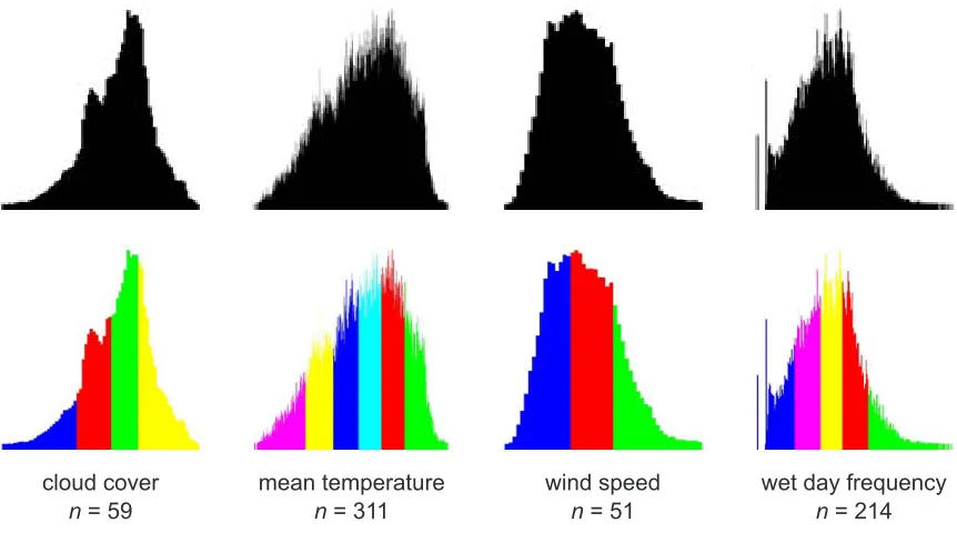
4.6 Discretizing Attribute Ranges . . . 51

4.7 Discretized Attribute Ranges . . . 52

5.1 Example of a Bayesian Network . . . 56

5.2 Types of Bayesian Networks . . . 60

5.3 Graphical Interest Rules . . . 73

6.1 Total Focus Event . . . 82

6.2 Capturing Elements . . . 85

6.3 View Wearing . . . 86

6.4 The Broad Focus View Volume . . . 87

6.5 Critique Interface . . . 90

6.6 Dataset Clustering . . . 94

6.7 Initial View Selections Before Adjustment . . . 96

6.8 Final Initial View Selections . . . 97

7.1 Pexel Visualization of the World . . . 99

7.2 Example A: Sequences 1 and 2 . . . 101

(9)

7.6 Example A: Final . . . 105

7.7 Example B: Sequences 1 and 2 . . . 106

A.1 Model Transformation . . . 127

A.2 Viewing Transformation and Clipping . . . 128

(10)

List of Tables

5.1 Simple Training Set . . . 65

5.2 Training Set with Uncertainty . . . 68

5.3 Weight Performances . . . 69

5.4 Interest Rules . . . 71

6.1 Weight Insertion . . . 80

(11)

Chapter 1 Introduction

1.1 Visualization and Navigation

Modern technology facilitates the collection and storage of large amounts of information.

To-day, the management of large datasets is both productive and profitable for a multitude of areas

such as e-commerce, library sciences, network security, natural sciences research, and

engi-neering. However, the ability to efficiently analyze and process data has struggled to keep

pace with the recent growth rates of datasets. It is difficult for humans to navigate or

under-stand the structure of large modern datasets. Consequently, locating interesting elements and

phenomenon is more challenging than ever.

Computers are a critical tool for the management and analysis of information. In computer

graphics, the area of visualization focuses on creating graphical representations of data to help

users acquire a more thorough understanding of a dataset. As opposed to raw data, humans

can process larger amounts of visual information at greater speeds. Visualizations support

analysis tasks such as determining relationships between data elements, detecting global or

local structure, and navigating within an information space.

(12)

amounts of information. Visualizations are built and organized with consideration towards

how the human visual system interprets an image. For example, psychology has identified

pre-attentive visual processing: the human ability to rapidly and accurately identify variations

in certain visual features such as color or shape from its background. By controlling these

same features, visualizations can quickly indicate outliers, boundaries, or clusters of elements

within a dataset. Visualizations rely on effective visual metaphors to display relationships and

structure. For example, high values are often associated with brighter colors, while low values

are associated with darker colors. Visualizations attempt to intelligently choose the best way

to render information depending on the user’s tasks and goals.

Visualizations address the increasing scale of data in a variety of ways. Some techniques

attempt to create effective contextual overviews for representing an entire dataset while

selec-tively displaying detailed information only about local regions. Other techniques try to reduce

or summarize the data while preserving its important features. Other techniques ignore the

scale issue and defer the management of large amounts of data to the user; i.e., they rely on

users performing navigation to explore select areas of the dataset.

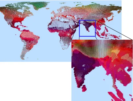
However, the effectiveness of most current visualization techniques remains susceptible to

datasets that exceed a maximum number of elements (see Figure 1.1). The resulting visual

representations are so large and complex that they become incomprehensible to the user and

prohibitive to simple navigation. To compensate, visualizations often place large portions of

information outside the user’s current view (i.e., off-screen). This further complicates

naviga-tion and inhibits user orientanaviga-tion by removing wayfinding cues from the user’s view. It also

hampers a primary goal of visualization: locating interesting data elements. Therefore, a

criti-cal problem for any visualization technique is efficiently locating and exploring this off-screen

information.

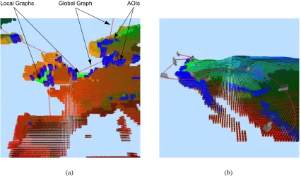
One alternative to creating new visualization techniques is to supplement existing ones with

(13)

en-Figure 1.1: A glyph-based visualization of global weather conditions. In the overview, details are occluded because of the dataset’s size, while the local view has relocated the majority of the dataset to outside the user’s view.

vironments. Mental maps allow users to accurately determine positions and perform efficient

wayfinding within a virtual world. Unfortunately, even with appropriate navigation support,

building accurate mental maps of large datasets can be a difficult, time-consuming task for

users. This is due to a number of reasons. First, a single view is often inadequate for showing

sufficient detail about a large environment. To build a proper mental map, large environments

must often be examined from multiple locations. By acquiring multiple perspectives, users will

better understand important positional relationships between distinctive features of the

visual-ization. Second, dense environments may contain significant amounts of noise that interfere

(14)

Centennial Parkway Western Boulevard A v ent F erry R o a d Centennial Campus Belk Tower Hillsborough Street State Fairgrounds Downtown Library Gym Main Campus Computer Science Building

Figure 1.2: The author’s mental map of North Carolina State University. There are three districts (Main Campus, Centennial Campus, and downtown), two landmarks (Belk Tower and State Fairgrounds), numerous nodes, major paths, and minor edges.

Lastly, dynamic environments complicate navigation, since important features and landmarks

potentially change their locations or appearances. As a result, existing mental maps become

obsolete and must be rebuilt.

Lynch claimed people form mental maps using environmental components such as edges,

paths, districts, nodes, and landmarks (see Figure 1.2) [76]. One way to construct a useful

navigation framework for a visualization is to build virtual equivalents of Lynch’s components.

These components should be based on data elements important to the user. For example,

elements of interest (nodes) can be clustered together into areas of interest (districts). Areas

of interest can then be connected to one another with a graph (edges and paths) to provide a

framework for building mental maps.

A critical issue of this scheme is identifying what parts of a dataset should act as the

compo-nents of this framework. Users are concerned with locating data elements exhibiting interesting

(15)

ele-ments. Thus, learning a user’s interests and reasoning with that information is a fundamental

problem for building effective navigation frameworks. This is a challenging problem because

interests are often user dependent, ephemeral, and unknown apriori.

One solution is requesting users to provide detailed descriptions of important properties

[27]. Any element matching these descriptions is automatically included in the framework.

However, this approach produces a static framework that only changes when users revise their

descriptions. Providing these descriptions can be an onerous task when a user’s preferences

are complex, extensive, or numerous. Thus, such a specification process will occupy time and

effort that could be better spent on exploring the data. A better framework would learn users’

interests as they explore a visualization and update the navigation framework based on their

interactions.

1.2 Preference Elicitation

Learning a user’s interests involves understanding how properties and data elements are

impor-tant to the user; i.e., identifying the user’s preferences. Preference elicitation is the process of

collecting preference information from users in efficient and non-influential ways. Preference

elicitation provides necessary information for developing accurate and beneficial user

prefer-ence models. These models are able to discriminate interesting elements from the rest of the

dataset. Research in areas such as artificial intelligence has developed many techniques for

representing user preferences and conducting efficient reasoning with these representations.

Preference elicitation techniques are focused on other aspects besides efficiently collecting

information about a user’s interest. They work to resolve conflicting preferences and address

how to make tradeoffs between competing user goals. They attempt to discover hidden

prefer-ences or erroneous user preference statements. Unlike other algorithms such as collaborative

(16)

an initial body of preference information.

Many preference elicitation techniques work in theory, but are unproven in real-world,

prac-tical applications. These algorithms have been implemented in environments especially suited

for the collection of preference information. These elicitation engines operate by repetitively

querying a user until they have acquired an adequate amount of preference data. It is unknown

how difficult it will be to modify these techniques to operate within an application not solely

focused on collecting preference information. In our case, we look specifically at visualization.

Visualizations are not designed to explicitly collect information about user preferences.

However, visualizations do share a similar goal with preference elicitation: locating interesting

and useful knowledge about a particular environment. This common goal provides important

connections for communicating preference information. An important issue is determining

how to modify these two techniques to co-exist effectively within the same environment. It is

unclear how a user’s behavior and interactions within a visualization context can provide the

information needed to construct a preference model.

1.3 Data Exploration

Integrating navigation techniques can improve visualizations designed for data exploration.

Data exploration is the process of analyzing a dataset in search of previously unknown and

interesting properties or elements within the data. When scientists create visualizations, they

often have general expectations about their data, but lack specific ideas of what they will find.

Rather, scientists explore visualizations hoping to find interesting phenomenon which might

not be easy to detect through standard mathematical or statistical analysis. Scientists often

arrive with broad interests about expected relationships and then proceed to look for unknown

specific values within their data. Such initial interests may change during the exploration

(17)

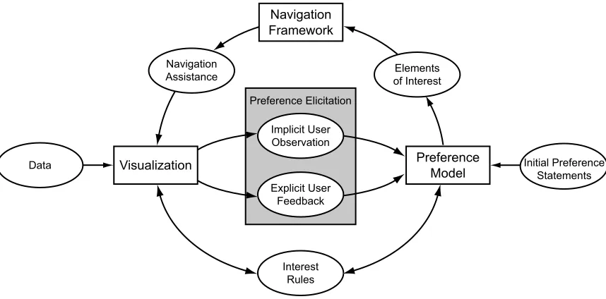
This thesis describes the creation of a more effective exploration system. This system is

composed of three primary parts: a visualization for exploring the dataset, a navigation

frame-work for wayfinding assistance to interesting areas, and a preference engine for identifying

in-teresting elements. The latter component dynamically identifies important areas in the dataset

while users interact with a visualization. Then, the system updates any existing navigation

sup-port and enables users to quickly locate any recently discovered off-screen regions of interest.

To accomplish this, the system must learn and model a user’s interests. This process involves

analyzing explicit feedback and interpreting user behavior.

There are many advantages to using such an exploration system. Automatically inferring

interest allows users to remain focused on exploring the dataset. Such systems can analyze

the state of a user model and generate the descriptions of what it believes is interesting even

when users cannot themselves explicitly describe their interests. Also, a computer can scan

and manage large data sets more efficiently than a human. It can quickly evaluate thousands or

millions of data elements within a visualization, while humans can examine only a few.

1.4 Research Goals

The overall goal of this work is integrating preference elicitation algorithms into visualizations

to create a more effective data exploration system. These elicitation techniques will provide the

necessary input for building a user preference model. This model will be used to automatically

and dynamically identify areas of interest within a visualization. In order to achieve this goal,

our system will implement the following components:

1. Create a revisable and iterative model of a user’s preferences that can be updated as new

preference information is collected. At any point in visualizing data, the model exists in

a state where it can attempt to determine if an element is interesting. Even with minimal

(18)

input is incorporated, the model will converge to a more accurate representation of the

user’s preferences.

2. Create or modify existing preference elicitation techniques and interfaces to collect

infor-mation from a user in parallel with visualizing the data. These tools and techniques will

minimize interference with the visualization process. The system can collect information

via explicit and implicit styles of elicitation.

3. Modify and format input collected by these mechanisms such that it is compatible with

the underlying user preference model. The types of preference input that can be collected

from a visualization often prevent a simple translation.

4. Integrate these components into an existing visualization and navigation system. This

new preference model and its complimentary techniques will improve an existing system

by making it a more dynamic and powerful tool for data exploration.

The remainder of this thesis is organized as follows. Chapter 2 provides a general

back-ground on visualization techniques and some of the challenges they face. Chapter 3 explores

the existing research on modeling and eliciting user preferences. Chapter 4 gives an overview

of the augmented visualization and navigation system. Chapter 5 describes the motivation and

selection of the chosen user preference model. Chapter 6 discusses how user input is collected

from a visualization and integrated into the underlying preference model. Chapter 7 provides

examples demonstrating how these techniques and the user model perform. Chapter 8

(19)

Chapter 2 Visualization

2.1 General Overview

A datasetDis a collection of data elements,D={e₁, . . . , e_N},whereN is known as the size ofD. Every elemente_iis an assignment of scalar values to an attribute setA ={A₁, . . . , A_M},

where M is known as the dimensionality of D. Thus, e_i = (a_i,1, . . . , a_i,M). These attribute variables may assume discrete or continuous values from either a bounded or unbounded range.

A visualization is the construction of a function mapping attribute values to visual features. The

challenge of visualization is finding good mappings to accurately represent the data.

Visualizations are often categorized as either information visualization or scientific

visu-alization. Information visualization is typically used to manage abstract data, or data lacking

any associated physical properties. Examples of abstract data include electronic documents,

network traffic, demographic information, user profiles, and e-commerce transactions. Often

information visualizations try to impose a meaningful geometry that emphasizes important

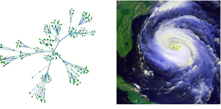
relationships within a dataset (see Figure 2.1a). Scientific visualization focuses on data

pos-sessing some inherent geometric structure (see Figure 2.1b). Examples of physically-based

(20)

(a) 3D Graph Visualization (b) Hurricane Fran Visualization

Figure 2.1: (a) is an example of an information visualization showing a hierarchy graph laid out in a radial manner within 3 dimensional space (courtesy of Steve Benford, University of Nottingham, UK). (b) is an example of a scientific visualization of Hurricane Fran. The image was built from data collected with a satellite (courtesy of NASA).

visualization are not mutually exclusive. Techniques from either area are used for representing

both abstract and physically-based datasets.

Visualizations rely on the strengths of the human visual system and common visual metaphors

for creating effective images. Visualizations incorporates research from areas outside of

com-puter graphics; for example, psychology, art design, and human comcom-puter interaction. By

studying how the human visual system interprets visual information, visualization researchers

can develop non-intuitive, effective representations of data (see Figure 2.2) [111, 101]. Also,

they maximize the use of other common visual properties such as color and texture [109, 110,

49, 50, 52]. By studying techniques used by artists and designers, visualizations can become

both effective and engaging representations of data (see Figure 2.5) [75, 53, 68].

While many visualization techniques succeed in creating graphical images that effectively

(21)

Figure 2.2: This visualization is based on a cognitive model that describes how the human visual system perceives orientations from a local configuration of dots [101]. Here, the model is used to visualize flow in simulated supernova data. Color corresponds to magnitude.

commonly found in modern datasets. Visualization must address the fundamental problem

of how to represent large amounts of information within a limited display. Consider how a

standard display device supports a 1280× 1024 pixel resolution, approximately 1.3 million

pixels, to represent datasets regularly containing many more data elements. Moreover, data

elements may be composed of multiple attributes, further increasing the demand on available

display resources. This forces information to be re-located “off-screen,” usually by way of

filtering or clipping mechanisms. Visualization techniques are designed to intelligently choose

(22)

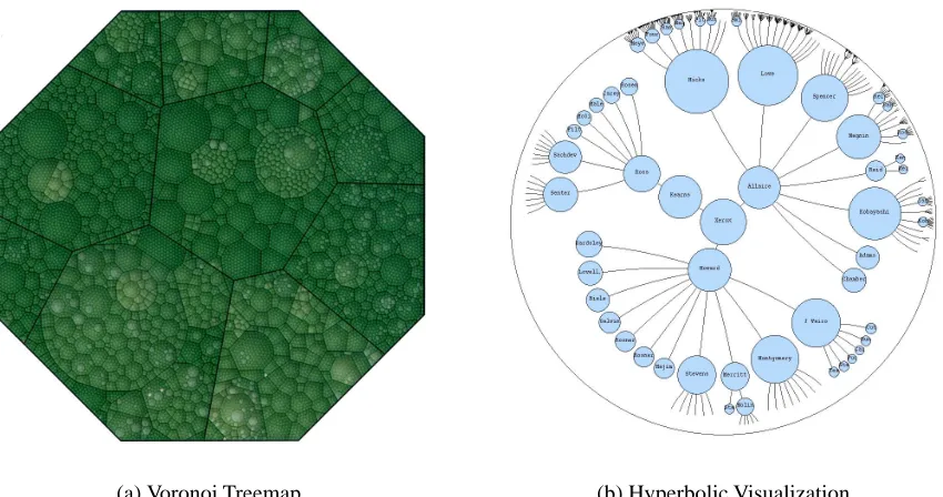
(a) Voronoi Treemap (b) Hyperbolic Visualization

Figure 2.3: (a) is a overview+detail visualization technique: a voronoi treemap visualizing a hierarchical structure with 16288 nodes and 7 levels. [5]. (b) is a focus+context visualization technique, the hyperbolic browser, displaying another hierarchical structure [72].

2.2 Large N

When visualizing a dataset with a large N, individual or groups of data elements must either be warped or removed from the user’s view in order to encapsulate the entire dataset within the

display. focus+context and overview+detail are two families of visualization techniques that

attempt to fit large numbers of data elements within a single screen. These techniques try to

balance displaying global structure with local detail in the user’s view.

overview+detail techniques create a global overview of the dataset while providing users

with interactive tools for accessing local, detailed information. Overviews are used to

effi-ciently search the dataset for interesting areas and to identify global structure. Meanwhile local

views provide more detail about individual data elements. These two views often compete over

screen time or display space. Therefore, multiple views are provided either at different times

(23)

multiplex-ing) [18]. For example, Lifelines contains an overview window of a patient’s medical history

and supporting local windows for accessing more details about particular aspects of the patient

medical history [89]. Semantic zooming enables users to transform their current view from a

general overview into a more detailed view [9, 10]. The treemap (see Figure 2.3a) lays out

local information to concurrently display the global structure of the data [99].

focus+context techniques present local information (focus) simultaneously with global

in-formation (overview), often in a single unified image. Many focus+context techniques warp

or filter data elements from the display. Elements close to a focal point are represented with

more detail than those further from the focus [39, 72, 77, 93, 94]. The fish-eye technique uses

a value function coupled with an element’s distance from the focal point to determine how,

if at all, to display a data element [38, 39]. The hyperbolic browser (see Figure 2.3b) maps

elements to a tree-structure in hyperbolic space. This space is projected onto a Euclidean disk

for exploration. The projection produces a warping effect similar to a fish-eye lens [72, 71].

These techniques provide effective ways of representing larger numbers of data elements.

However, they are still ineffective for very large datasets. Once their thresholds are reached,

the introduction of additional data elements create cluttered visual representations.

Visual-izations of large datasets may be thought of as large virtual worlds. Unfortunately, most of

these techniques do not provide any navigation support for exploring these worlds. As a

re-sult, users may become “lost” and unable to successfully traverse from one location to another.

Moreover, these techniques do not account for the complications associated with visualizing

multidimensional data elements.

2.3 Large M

Multidimensional datasets pose related, but somewhat different, problems. Data elements

(24)

rep-resented at the same spatial location. Multidimensional visualization techniques have been

categorized into five types [112]:

1. Brushing techniques allow users to reveal additional information about multidimensional

data elements when they are highlighted with a “brush” [8, 108].

2. Panel Matrix representations, such as the HyperSlice and hyperbox, create two

dimen-sional plots of different attribute values [3, 105]. These plots are presented alongside

each another for the user to analyze.

3. Hierarchical displays organize multidimensional data into a hierarchical structure

pos-sessing different levels of display [32, 31, 80, 81].

4. Non-Cartesian displays construct new axes on which to plot data attribute values [57, 65,

64]. These displays provide representations that simplify the detection of relationships

between data attributes.

5. Iconography uses collections of icons or glyphs to represent multidimensional data [43,

51, 50, 88, 110]. These glyphs often use texture properties to represent multiple data

attributes at the same location.

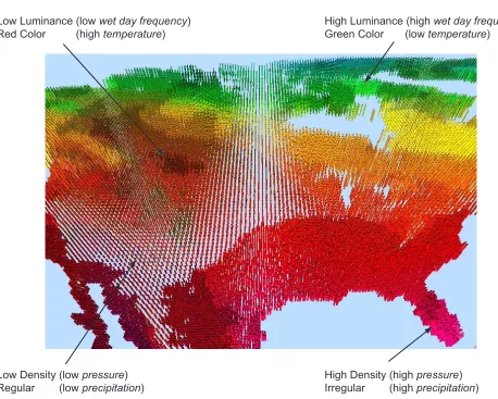
Iconographic visualization techniques map data attributes to visual features. Attribute

val-ues stored in a data element can then be used to vary the visual appearance of an elements’s

glyph. Examples of common visual features include color, density, height, regularity, and

ori-entation, etc (see Figure 2.4). The human visual system can perceive and process different

degrees of variance among these visual features. For example, there are seven different color

values and three different densities that the human visual system can rapidly and accurately

identify [49, 51]. Visual features sometimes interfere with one another. Therefore, effective

(25)

Figure 2.4: (b) shows the use of texture to represent the weather conditions of the United States [50]. Height, color, regularity, and luminance visual features are mapped to the weather attributes wind speed, mean temperature,

precipitation, and wet day frequency, respectively.

As the number of dimensions of a dataset increases, the number of visual resources required

to render each data element also increases. Multidimensional visualization techniques focus on

how to best represent multidimensional data. They are not as concerned with the total number

of elements to be displayed and assume there will be an adequate amount of screen space for

the resulting image. As elements compete for display resources, information becomes clipped,

(26)

Figure 2.5: This image shows properties of two dimensional flow about a cylinder [69]. Arrow size and direction correspond to the magnitude and direction of the flow, vorticity corresponds to the background color, and ellipsoid properties correspond to divergence and shear. Additional rectangular glyphs correspond to turbulent charge and

(27)

Chapter 3 Preferences

3.1 Decision Theory

The goal of preference elicitation is to facilitate the construction of an accurate user model.

This model is used by a decision support system to assist a user with the completion of a task.

Preference elicitation is designed to provide the necessary data for the relevant decision support

framework. The theoretical foundation forming the basis of these models is found in decision

and utility theory [63, 34]. Decision and multi-attribute utility theory focus on the evaluation

of choices and outcomes for a decision problem or scenario.

Outcomes are defined by the assignment of values to a set of attribute variables, X =

{X₁, ..., X_n}. Attribute variables are either discrete,x_i ∈ {x_i,1, ..., x_i,m}, or continuous,x_i ∈

[a, b]. The set of outcomes O considered for a decision problem is contained by the outcome

space Ω. Typically, Ωis defined by the Cartesian product of X. Thus, O ⊆ Ωwhere Ω = {X₁×X₂×...×X_n}. Consequently, it is common forO to be very large. Even an outcome space composed of discrete attribute variables has the potential to be combinatorially large.

For many scenarios, Ω contains outcomes infeasible in the context of the current decision

(28)

{X_α, X_β}, each variable corresponding to one of two separate auction agents, αand β. The value ofX_αorX_β is a possible assignment of goods from the set{A, B}to the corresponding agent. Therefore, x_α, x_β ∈ {∅, A, B, AB}. An outcome o ∈ Ω has the form o = {x_α, x_β}. One potential value iso = {∅, AB}, corresponding to agent α receiving nothing and agentβ

receiving everything. Obviously, any allocation where both agents acquire the same good is

infeasible (e.g.,o ={A, AB}) and should not be considered by a decision maker. However, in practice,Ωwill remain very large, even with the removal of infeasible outcomes.

In order to make decisions based on a set of outcomesO, a decision maker often simply needs an ordering of the outcomes determined by the user’s preferences. This is called a

preference relation and is denoted by . Given o_i, o_j ∈ O, if o_i o_j, o_i dominates or is preferred too_j. Typically, the preference relation is induced by a value function,v(o) :O →R. For a given value functionv and its induced preference relation,, the following is true,

∀o_a, o_b ∈O, o_a o_b ⇐⇒ v(o_a)≥v(o_b).

Value functions operate on the set of outcomes or subsets of the attribute variables

them-selves. The value for a given attribute variable dominates another value if the following holds

true,

∀a, b∈ X_i, a b ⇐⇒ v(a)≥v(b).

Value functions reflect how much acquiring a particular outcome is worth to the user.

How-ever, in many decision scenarios there may exist a degree of uncertainty. Choosing one action

may result in receiving outcomeo₁with probabilityp₁or outcomeo₂with probabilityp₂. Since any one action no longer guarantees a particular outcome, the value function alone is

insuffi-cient for modeling a user’s decisions in scenarios with uncertainty. Users need a more complex

(29)

incorporate a user’s attitudes about risk along with their valuations of outcomes [63].

A main contribution of utility theory is a theorem proving the existence of a utility function,

u(x) :O →R. This function induces a unique preference relation,, overO. Unfortunately, a preference relation does not necessarily induce a utility function over the set of outcomes

because the utility function must also account for the user’s attitudes about risk. It is common

for the utility function to be equivalent to the user’s value function, especially in scenarios

without uncertainty. However, this is not a guaranteed condition. Utility functions also induce

a preference ordering on the probability distributions (or lotteries) over the outcome space. Let

P r_i andP r_j be two probability distributions over the outcomes caused by invoking either of two actionsa_ianda_j. Then,

a_i a_j ⇐⇒ X

o∈O

P r_i(o)u(o)≥X

o∈O

P r_j(o)u(o)

for the utility functionu. When assigning values for an outcomeo, the utility functionumust consider the uncertainty of attainingoand the user’s attitudes toward risk to correctly preserve the user’s preference relation for actions. The above relation implies that a user will prefer

the action resulting with the maximum expected utility (MEU). Elicitation systems assume the

user is rational; i.e., the user prefers the outcome with the maximum expected utility over all

other outcomes. For some decision problems, there exists a single utility function for a group

of users, while other problems mandate a unique utility function for each user.

Because the utility function for the user is frequently unknown apriori, constructing the

utility function is often the first step in building a decision support system. However, this is

a difficult task because building a complete utility function may require a full description of a

user’s preferences. Such a specification may be unavailable and difficult to acquire. The main

goal of preference elicitation is retrieving this information to build a user’s utility function and

(30)

3.2 Challenges of Elicitation

Despite the challenges of building an accurate and effective user model, eliciting preference

information alone is a non-trivial task. Many considerations need to be made by a system,

or elicitor, during the elicitation of preference information. Otherwise, systems may

inaccu-rately model the user, collect erroneous information, or unintentionally influence the user’s

preferences [12].

Having a user fully specify his preference order ab ovo is typically impractical for a number

of reasons. First, the potential number of outcome pairs the user must examine is a function

of the size of the outcome space. In the best case, an outcome space with discrete variables,

the outcome space grows combinatorially with respect to the number of attribute variables and

values. However, outcome spaces composed of even a small number of variables can generate

far too many comparisons for the user. Spaces with the infeasible outcomes removed still

may require prohibitive amounts of time and effort on a user’s behalf. Research has shown

that acquiring the right partial preference information can be as effective as having a user’s

complete utility function [47, 56].

Second, preferences are sometimes dynamic and ephemeral. It is common for different

users to have varying preferences. Often, users share some common preferences that can be

used as a reference or starting point for the elicitation process. Elictors must be prepared

to deal with each user on an individual basis, while maximizing the use of known common

preferences. Another important factor is users may change their preferences while they interact

with a system. As the user performs a task, old preferences may give way to new ones. Elicitors

need to be able to detect this change and make the appropriate adjustments.

Pu et al describe another important issue that preference elicitation techniques should

ad-dress [90]. Given the elicitation scheme, a particular choice of attributes may force users to

(31)

consider a traveler who is looking to take a long weekend trip to New York. He wishes to

restrict the amount of money he spends on airline tickets to only 300 dollars (his fundamental

objective). If an elicitation scheme asks him how much he is willing to spend on his departure

ticket, the traveler is forced to form a means objective. If he estimates to spend equal amounts

of money on both departure and return flights, specifying 150 dollars would exclude a

poten-tially optimal outcome of a 200 dollar flight into New York on Thursday afternoon paired with

a 75 dollar red-eye return flight on Sunday night. Elicitors must provide users with ways to

state their fundamental objectives.

Furthermore, it has been shown that the method of elicitation can influence how users

re-spond to elicitation [12]. Users may accidentally misinform the system about their preferences.

Elicitors try to prompt the user as infrequently as possible to keep users focused on their

pri-mary tasks. Well-designed queries provide the highest yield of preference information while

simultaneously reducing any error in the model.

Incremental preference elicitation attempts to satisfy the above criteria by intelligently

de-ciding how to subsequently elicit the user based on information already collected. Incremental

elicitation techniques do not always have initial preference information about the user. This is

the case with many scenarios. Incremental elicitation allows users to revise their preferences

as they interact with a decision support system. Such functionality is not possible with systems

requiring full elicitation before the decision making process begins.

3.3 Types of Queries

The first step to eliciting preference information is determining the form of the questions

sub-mitted to the user. Elicitation queries provide an elicitor with appropriate information for

im-proving its understanding of a user’s preferences. Elicitation queries need to be simple enough

(32)

The simplest way to discover a user’s preference relation is requesting the user to compare

two possible outcomes. These are order queries and they often have the form of “Do you

prefero_a oro_b?” Many models assume that preferences are transitive: ifo_a o_b ando_b o_c

then o_a o_c. If transitivity holds across a user’s preferences then order queries can provide a great deal of information about preference. Otherwise, order queries become an inefficient

elicitation query because they only reveal local relationships about different outcomes. Another

disadvantage to order queries is that they only provide an ordering of the outcomes. There

is no quantitative result describing how much a user prefers one outcome to another. Order

queries only provide qualitative information about the user’s preference relation and can not

fully determine the user’s value function. However, it is often easier for users to choose the

preferred outcome when compared with another instead of specifying absolute numeric values

for each outcome.

Rank queries are a more specific type of order query. They request users to explicitly rank

an outcome among all other outcomes. Rank queries may have the form “What is the rank of

o_a?” or “What outcome has rank r?” These queries are not always feasible since the set of outcomes is possibly too large for users to produce accurate rank values. Used in conjunction

with order queries, rank queries are good for quickly approximating where a given outcome

resides in the preference relation.

Value queries provide a quantitative measure of preference between outcomes. They

es-tablish how much a user prefers one outcome to another; i.e., a quantitative preference value.

They might be of the form “What is the value for outcomeo_a?” The ability of a user to truth-fully answer a value query often depends on the size of the set of outcomes. It is difficult for

users to compute accurate values for individual outcomes when dealing with a large number of

outcomes.

A variation of the value query is the standard gamble query. The standard gamble query

(33)

willing to make in order to acquire this particular outcome [83]. The standard gamble query

is common among decision theory research because it provides exact information for very

accurate revisions to the preference model. The standard gamble query has the following form:

Consider three outcomeso_a,o_b, ando_c, where it is known the user’s preference ordering exists such thato_a o_b o_c. A standard gamble query asks if the user prefers to definitely acquire

o_b or accept a gamble (or lottery) where the user acquires o_a with probabilityπ or o_c with probability(1−π). Utility theory guarantees a value forπwhere the user is indifferent between acquiringo_band accepting the gamble. The value ofπfor which the user is indifferent between the gamble and the outcomeo_bdetermines the normalized utility value ofo_b: u(o_b) =πu(o_a)+

(1−π)u(o_c). Typically, the best and worst case outcomes are used foro_aando_b. Ifu(o_best) = 1

andu(o_worst) = 0, the aforementioned formula easily shows that π is the value of the utility function foro_b.

Potential outcomes or solutions are another form of queries used to determine the

prefer-ences of the user. This type of elicitation is often search-driven. Users move through a solution

space evaluating possible candidates chosen by the system. How the user responds to potential

candidates determines the selection of future candidate optimal outcomes. Search is driven by

having the user indicate the specific properties preferred or disliked from the given examples.

3.4 Preference Structure

Given that even the size of outcome spaces composed of only a few attributes is potentially

large, decision support systems must take advantage of any structure inherent to the user’s

preferences. Considering preference structure facilitates an efficient interaction between the

system and the user by reducing the amount of information the user must provide. Decision

theory describes various forms of structure found in preferences. Most of these forms are a

(34)

problem piecemeal [63, 4]. In other words, identifying independence reduces the number of

outcomes for the user’s examination by decreasing the number of independent combinations

of attributes for consideration. Independence also allows for the construction of less complex

and more structured utility functions.

The most basic form of independence is preferential independence. Preferential

indepen-dence considers only the preference ordering over the individual outcomes for a decision

prob-lem. A set of attributesY ⊂ X is preferentially independent ofX −Y when the preference order over outcomes with varying values of attributes inY does not change when the attributes ofX−Y are fixed to any value; i.e., the preference order of outcomes with attribute values in

Y does not depend on the values of attributes inX−Y. Letαbe an assignment of values to the attributes inY andγ be an assignment of values to attributes inX−Y. IfY andX−Y are preferentially independent then everyx ∈ X has the formx = (α, γ). Formally, preferential independence is defined as

∀γ, γ0 ∈(X−Y) : (α, γ)(β, γ) ⇐⇒ (α, γ0)(β, γ0)

withα, β ∈Y.

Utility independence is concerned with the utility function as well as the user’s preferences

among the outcomes. Not only must the induced preference relation stay unchanged, but the

user’s attitude about risk or the relative strength of preference between outcomes must also

remain the same. To understand utility independence, the notion of conditional preference

must be described. For a conditional preference relationwithY ⊂ X, letα andα0 be two assignments of values to the attributes inY. IfZ ⊆ X−Y, letγ be an assignment of values to the variables inZ. αis conditionally preferred toα0 with respect toγ if

(35)

Conditional preference can also be applied to probability distributions over outcomes. Using

the same assignments for Y and Z described above, consider a probability distribution Pr overX. There exists a unique distribution Prγ _{such that the marginal probability of Pr}γ _(the

probability that the attributes ofZ take the values ofγregardless of the values of the attributes in Y) over Y is Pr and Prγ _{gives the probability of 1 to the values of} _γ_{. Given a utility}

function with its associated preference order , the conditional preference over X given γ, γ, is defined as

Pr_a_γ Pr_b ⇐⇒ Prγ_a Prγ_b

for two probability distributions Pr_aand Pr_boverX.

With the definition of conditional preference established for probability distributions over

the set of outcomes, it is possible to state a concrete description of utility independence. IfX =

(Y, Z),Y is said to be utility independent ofZ if the conditional preferences for distributions overY given an assignment of valuesγ to the attributes inZ are independent of the particular values ofγ. Moreover, it is known thatY is utility independent ofX −Y if and only if the induced preference structure’s utility function has the form,

u(X) =f(X−Y) +g(X−Y)h(Y)

for a positive functiong[4]. A utility function in this form is an improvement since the number of independent values to collect is fewer than the number required of preference structures with

dependent structure.

A stronger independence can be identified in a preference structure if the following

(36)

additive independent. A set of variables for an outcome space which is additive independent

has a utility function of the form

u(X) =

k

X

i=1

f_i(X_i)

where f_i is considered the utility function for the attribute X_i, also known as the subutility

functions.

Independence among attributes is important to preference elicitation because it allows the

creation of more efficient elicitation techniques and interfaces. Given the potentially large

number of outcomes a decision problem can create, independence among attributes allows

elicitors to refine the set of potential queries needed to build an accurate representation of the

user’s preferences. Also, elicitors can identify the important attributes and focus queries on

their values. For preference structures with additive independence, Keeney and Raiffa provide

a procedure for reducing the number of queries by creating scales for each of the components

of the utility function and querying the user about the behavior of each subutility function [63].

Then, variations of the standard gamble and value queries are used to construct the appropriate

scaling constants,k_i.

Chajewska and Koller work to construct more generalized factorizations of a utility

func-tion. They treat utility functions as random variables and create a statistical model of the

expected utility function. Their model assumes the population of users can be segmented into

subpopulations. Members of the subpopulations typically have similar utility functions, thus

allowing the creation of a probability density function over a subset of the variables ofX. Let

C be a set of clusters formed with variables from X, C = {C₁, . . . , C_m} where C_i and C_j

for every i and j are not necessarily disjoint. Then, a utility function is said to be factored

according to C if there exists a function u_i : Dom(C_i) → R such that the utility value of

(37)

functions are the subutility functions. Note, that this “factorization” allows for multiple clusters

to share variables inX, a condition not permitted with additive independence. The statistical model creates a subutility function for each subpopulation and then uses this function for

guid-ing the elicitation process. Unfortunately, this work depends on the existence of a pre-existguid-ing

database of user utility functions.

Perhaps the most important contribution of independence from an intuitive aspect is it

al-lows the construction of simple and manageable utility functions. For additive independent

attributes, the user’s utility for any given outcome can be broken down to the sum of values

for individual attributes. Instead of a utility function withn parameters, the system now has

nutility functions with one parameter. Revision of the utility function takes place at the most atomic level: the attributes. It can be accomplished by manipulating scaling constants and the

value of the utility function for each attribute value. Here, changing the utility function with

respect to one attribute has no impact on the other attributes’ utility functions. Thus, systems

can revise one attribute at a time. This simplifies interface design and allows users to more

easily evaluate outcomes.

3.5 Preference Representation

The elicitation process often depends on how a user’s preferences are represented in the

sys-tem. The representation structure determines what information the elicitor retrieves and the

sequence in which it is collected. The representation of a user’s preferences is typically

asso-ciated with modeling the user’s utility function. Since many decision scenarios manage

multi-attribute problems, most representations are capable of expressing the user’s preferences over

multidimensional datasets. These representations tend to be either vector-based, graph-based,

(38)

3.5.1 Vector Models

Vectors are fundamentally simple representations for preferences. The content of vector

rep-resentations depends on the particular elicitor. Some systems create a vector of length|O|and store the values or utilities of every potential outcome. Evaluating the utility of a particular

out-come involves referencing the corresponding index of the vector. In order to adjust the value of

the utility function, the vector’s values are updated accordingly. These vectors explicitly model

the entire domain and range of the utility function [14, 21, 19, 46]. Vectors provide a

deter-minate representation of the utility function, offering little information about how the utility

value was computed for any given outcome. Consequently, vectors do not explicitly represent

any inherent structure within the preference relation. However, there do exists algorithms for

vector representations that detect preference structure [20].

Sometimes vectors store components of a decision problem; i.e., attribute values or

con-straints. The utility value for an outcome is computed with a subset of the vector’s entries.

The Automated Travel Assistant maintains a vector of constraints and a vector of weights [74].

Each constraint is a function C_i(x) : dom(X_i) → [0,1], where C_i(x) = 0 implies the con-straint is fully satisfied andC_i(x) = 1means the constraint is fully unsatisfied. ATA assumes the preference structure’s attributes are additive independent. The authors use these

defini-tions to construct an error function. This function provides an antipodal utility function and

measures how unimportant a given outcome is for a user,

error(|x₁, . . . , x_n|) =

n

X

i=1

w_iC_i(v_i)

where w_i is a weight ranging from[0,1]forC_i. As the user provides additional information about the values ofC_i andw_i, the vector is updated and the error function begins to approach zero; i.e., the constraints more accurately represent the user’s preferences. ATA allows for

(39)

ATA models user preferences as a Constraint Solving Problem (CSP). CSP preference

rep-resentations have been used in a variety of systems [15, 17, 74, 97, 103]. Upon acquiring

an adequate set of constraints, C, constraint solving routines can determine any potentially optimal solutions. IfC is not tight enough to eliminate the majority of candidates, additional constraints are elicited from the user. In many traditional CSP solvers, constraints are hard; i.e.,

either fully satisfied or not. When no outcome satisfies the entire set of constraints, CSP solvers

relax some constraints to find an optimal solution. Hard constraints alone may be inadequate

for modeling preferences, since it is possible for users to have conflicting preferences. Ranking

a set of hard constraints helps with determining the order in which to relax constraints.

Rank-ing also implicitly creates an assignment of importance weights. These weights can model how

strongly an outcome satisfiesC. This is helpful in scenarios where a user’s utility for a few highly-ranked constraints may be surpassed by the utility of a larger number of lower-ranked

constraints. The use of soft constraints offers even greater flexibility because they model the

degree to which an outcome satisfies a set of constraints. This quantitative measurement is

typically the sum of the products of an importance weight with a satisfaction value for each

constraint. This technique is very similar to the error function of ATA.

3.5.2 Graph-based Models

Network-based and graph-based structures are another method for representing user

prefer-ences [4, 13, 24, 23, 48]. The topology of these structures assists with realizing preference

structure by contributing a visual representation of how outcomes are dominated by other

out-comes. Nodes of these structures are typically attribute values, but may be other appropriate

entries, such as outcomes. Thus, graph-based models can provide a more intuitive

representa-tion than vectors.

(40)

structure [25]. Preference structures tend to be transitive; i.e., if o_a o_b and o_b o_c then

o_a o_c. However, some decision scenarios allow for o_c o_a. It is difficult to construct a single, consistent utility function whose output can successfully represent an intransitive set of

preferences. Graph-based models can show this by creating cycles in the underlying graph.

Graph-based models can also reveal independence within a user’s preferences. Bacchus and

Grove explored a graph-based representation of utilities exhibiting a weaker form of additive

independence, called conditional additive independence [4]. This work helps decompose a

utility function into smaller subcomponents which are constructed with subsets of the attribute

space. These subsets are not necessarily mutually exclusive.

Boutilier et al created a network to capture and represent conditional preferential

inde-pendence [13]. A conditional preference network (or CP-network) creates a node for every

attribute X_i. For every attribute X_i, the user must identify a set of parent attributes whose values influence the preferences over the values ofX_i. Each node,n_i, has an associated table describing how the parents’ values affect the preference for the value of X_i. Using a set of initial conditional preference statements, a CP-network can rapidly determine which of two

outcomes dominates the other, or if there is insufficient information to determine the dominant

outcome. In the latter situation, the CP-network will identify an outcome whose preference

information will fill the necessary gap in the CP-network’s logic.

Conen and Sandholm make use of graph-based structures to store preference information

for a combinatorial auction setting [24, 23]. They build an augmented order graph which

is composed of a node for every possible bidder and bundle; (i.e., a subset of the items up

for auction). A feasible allocation (an outcome) is a set of nodes from the augmented order

graph where no two nodes represent the same agent and no two nodes have bundles containing

the same item. Algorithms use the augmented order graph to determine the set of

Pareto-optimal allocations. An allocationAis Pareto efficient if there is no other allocationB where

(41)

represents the bundle allocated to agentibyA). The graph can also be used to collect welfare-maximizing allocations: an allocation A where Pn_i=1v_i(A_i) is maximized among all other allocations. Using the set of welfare-maximized allocations, value information can be elicited

from the user to reduce the set of candidate allocations and find the optimal solution.

3.6 Selecting the Next Query

Elicitation queries are designed to reveal relevant information about preferences of the user.

Intelligently building a proper sequence of questions makes elicitation an efficient process.

Elicitors try to collect the largest amount of preference information with the least number of

questions. Therefore, elicitors choose the sequence of preference queries with consideration.

3.6.1 Metric Techniques

The most intuitive technique is creating a metric that evaluates the usefulness of potential

ques-tions. Various research projects have adopted a value of information metric which measures

the expected improvement in preference information after incorporating the answer to a given

query. The form of the value of information function depends on the decision support system.

Given a potential query, Chajewska et al compute the expected utility of the corresponding

outcome when each possible answer is factored into the utility function [21]. The new utility

values are also weighted by the likelihood of a particular answer from the user. This likelihood

is specified by a statistical model of the user. The average of the potential utilities minus the

current expected utility defines the value of information for any query. Unfortunately, this

func-tion only computes a myopic value of informafunc-tion; i.e., it does not consider the consequences

of future queries. Computing the full value of information is intractable and requires the

look-ahead consideration of all possible future combinations of questions and answers. [14] extends

(42)

the elicitation process. This approach analyzes the value of sequences of questions before

recommending the next query.

Boutilier et al adopt a similar metric technique for their decision scenarios [13]. For a given

decision scenario with potential actionsa_i, they examine the amount of regret a given action might receive. Factoring uncertainty into their model, the expected value of a given actiona_i

(for the elicitation context an action issuing a query to the user) is defined as

EV(a_i, w) =X

o∈O

P r_i(o)u(o, w)

for a given a distribution of tradeoff weightswfor the utility function. Definea∗_w as the action with the highest expected value; i.e., a∗_w is currently the best action to take for this decision problem. The regret ofa_iwith respect towis defined as,

R(a_i, w) =EV(a_w∗, w)−EV(a_i, w)

which is a measurement for the loss incurred by performing a_i instead of the optimal action

a∗_w. UCP-networks are used to form a set of linear constraints for the possible tradeoff weight values. These constraints define a subset of the distributions over outcomesOdenoted asC.

For a given set of constraintsC, the maximum regret of actiona_iwith respect toCis defined as

M R(a_i, C) = max_w_∈_CR(a_i, w)

The set of constraints are modified using queries with a finite number of responses to minimize

(43)

the regret-based query selection process.

Ha and Haddawy use a metric in their work called the rank correlation coefficient [45].

They needed a technique to measure the difference in the importance rankings of attributes

between two different strategies. Considering permutations of the forma=a₁, a₂, . . . , a_nand

b=b₁, b₂, . . . , b_n, the rank correlation coefficient is defined as

ρ(a, b) = 1− 6

P_n

i=1(ai−bi)2

n3−n

where the range of ρ is −1 ≤ ρ(a, b) ≤ 1. A value of 1 corresponds to two permutations being identical, while a value of -1 corresponds to a complete reversal of rankings. The rank

correlation coefficient is used to identify the two potential strategies whose rankings differ the

most from one another. Then, the system elicits the user for information on how to merge the

preferences of these two strategies into a single new strategy. By merging strategies, the system

reduces the number of candidate strategies for the user’s consideration.

3.6.2 Providing Examples

A major disadvantage of some valuation techniques is how they force users to examine and

make statements about attribute values out of context. Moreover, making such detailed

state-ments can be difficult for a user with underdeveloped or generalized preferences. One solution

is using general preferences to isolate a set of candidate examples from the outcome space.

Users modify the preference model by examining and providing feedback about these

exam-ples.

Providing examples to the user, or exampling, is perhaps the most intuitive way for users

to provide preference information. Users have the ability to rapidly return accurate feedback

about candidate solutions. They inform the system about which attribute values they like or

Integrating Preference Elicitation into Visualizations

INTEGRATING PREFERENCE ELICITATION INTO VISUALIZATIONS

BRENT M. DENNIS

COMPUTER SCIENCE

Contents

List of Figures

List of Tables

Chapter 1

Introduction

1.1

Visualization and Navigation

1.2

Preference Elicitation

1.3

Data Exploration

1.4

Research Goals

Chapter 2

Visualization

2.1

General Overview

2.2

Large N

2.3

Large M

Chapter 3

Preferences

3.1

Decision Theory

3.2

Challenges of Elicitation

3.3

Types of Queries

3.4

Preference Structure

3.5

Preference Representation

3.5.1

Vector Models

3.5.2

Graph-based Models

3.6

Selecting the Next Query

3.6.1

Metric Techniques

3.6.2

Providing Examples