On the Evolution of Mutation in Changing Environments: Recombination and Phenotypic Switching

DOI: 10.1534/genetics.110.123620

On the Evolution of Mutation in Changing Environments:

Recombination and Phenotypic Switching

Uri Liberman,*

,†

_{Jeremy Van Cleve}

‡,1

_{and Marcus W. Feldman}

‡,2

*School of Mathematical Sciences, Tel Aviv University, Tel Aviv, Israel 69978,†Holon Institute of Technology, Holon, Israel 58102 and‡Department of Biology, Stanford University, Stanford, California 94305-5020

Manuscript received September 27, 2010 Accepted for publication December 13, 2010

ABSTRACT

Phenotypic switching has been observed in laboratory studies of yeast and bacteria, in which the rate of such switching appears to adjust to match the frequency of environmental changes. Among possible mechanisms of switching are epigenetic influences on gene expression and variation in levels of meth-ylation; thus environmental and/or genetic factors may contribute to the rate of switching. Most previous analyses of the evolution of phenotypic switching have compared exponential growth rates of non-interacting populations, and recombination has been ignored. Our genetic model of the evolution of switching rates is framed in terms of a mutation-modifying gene, environments that cause periodic changes in fitness, and recombination between the mutation modifier and the gene under selection. Exact results are obtained for all recombination rates and symmetric fitnesses that strongly generalize earlier results obtained under complete linkage and strong constraints on the relation between fitness and period of switching. Our analytical and numerical results suggest a general principle that recombination reduces the stable rate of switching in symmetric and asymmetric fitness regimes and when the period of switching is random. As the recombination rate increases, it becomes less likely that there is a stable nonzero rate of switching.

I

N large populations subject to mutation between alleles under selection that is constant over time, mutation–selection equilibria can be stable. In the neighborhood of such a stable equilibrium, if an allele at a locus that controls the rate of mutation is intro-duced, this allele will invade if it reduces the mutation rate (Liberman and Feldman 1986). This is one ex-ample of the reduction principle for constant selection regimes (Feldman and Liberman 1986). This ap-proach, using the selectively neutral genetic modifiers of parameters such as mutation, recombination, and migration that are important features of the evolu-tionary process, can be viewed as an alternative to an approach using evolutionary stable strategies (ESS) (Maynard Smith 1978) or to finding critical points of the mean fitness (Karlin and McGregor 1972, 1974).

It has become usual to denote the gene on which selection occurs directly as the major gene (or in the case of recombination modification, genes) and the locus that controls the parameter of interest as the mod-ifier gene (e.g., Feldmanet al.1997). If a new mutation at the modifier gene is introduced during a transient

phase of evolution, rather than near an equilibrium, the fate of the modifier mutant may be quite different: for example, an allele that causes reduction of recombina-tion will succeed if it is introduced near stable linkage disequilibrium, but if it arises at a phase of the dynamics where the major loci are proceeding toward fixation, increase of recombination may occur and the reduction principle does not necessarily hold (Maynard Smith 1980, 1988; Bergmanand Feldman1990). The evolu-tion of modifiers of mutaevolu-tion, recombinaevolu-tion, or migraevolu-tion rates when the regime of selection on the major gene(s) is not constant over time has seen far less mathematical or even numerical analysis than the case of constant selection. Early numerical work by Charlesworth (1976) showed the failure of the reduction principle for recombination under some patterns of cyclically fluctuating abiotic selection.

Host–parasite systems may produce cyclical dynamics that have features similar to those of cyclically fluctu-ating abiotic selection. The evolution of host recom-bination in a host–parasite cyclical system has been addressed by Hamilton (1980) and most recently by Gandonand Otto(2007). Hamilton used a mean fit-ness argument to demonstrate an advantage to hosts with higher recombination, and Nee(1989) used a sim-ilar approach in finding that mutation rates should in-crease in both host and parasite. Gandon and Otto (2007) showed that alleles at a recombination-modifying locus that increased recombination could succeed Supporting information is available online athttp://www.genetics.org/

cgi/content/full/genetics.110.123620/DC1.

1_{Present address:Santa Fe Institute, 1399 Hyde Park Rd., Santa Fe, NM}

87501.

2_{Corresponding author:Department of Biology, Stanford University, 385}

Serra Mall, Stanford, CA 94305-5020. E-mail: [email protected]

in such host–parasite models. Mutation-increasing al-leles may be favored in similar models, as shown by Haraguchi and Sasaki (1996) and M’Gonigleet al. (2009). The latter authors also showed that under host– parasite cycling, increasing recombination between the mutation modifier and the gene under selection in the host decreased the stable mutation rate.

With increasing empirical interest in epigenetics, there has been a flurry of activity surrounding ‘‘stochas-tic switching,’’ a phenomenon observed in some studies of Saccharomyces cerevisiae, Escherichia coli, or Bacillus subtilis, where individual cells switch cyclically between different inheritable phenotypes (Thattai and van Oudenaarden2004; Kusselland Leibler2005; Acar

et al.2008). For example, experiments by Balabanet al. (2004) show that switching between phenotypes may differ between different genetic strains ofE. coli. The same group analyzed a mathematical model of this system and showed that the optimal rate of phenotypic switching was strongly dependent on the frequency of environmental changes but only weakly dependent on the strength of selection in any single environment (Kussellet al.2005). Earlier theoretical treatments by Ishiiet al.(1989) and Lachmannand Jablonka(1996) also found that optimal switching rates depended on the distribution of environmental periodicities.

Phenotypic switching may be an example of an epi-genetic effect, for example based on methylation (Lim andvanOudenaarden2007). There is some discussion as to the fraction of such epigenetic effects that are transgenerational (e.g., Youngsonand Whitelaw 2008) and, to the extent that they are, what their evo-lutionary effects might be (Bonduriansky and Day 2009). Most theoretical treatments of phenotypic switching have assumed that the organism is asexual and that the numbers of individuals grow exponen-tially (e.g., Kussell et al. 2005, p. 1809; Gaa´ l et al. 2010). These studies usually do not specifically include genetic contributions to the rate of switching; excep-tions are the analyses by Ishiiet al.(1989) and Salathe´

et al. (2009), both of which took fitness to be the phenotype that switches and allowed the rate of switching to be under the genetic control of a muta-tion-modifying locus. If switching is epigenetic and heritable, it is reasonable to propose that it is at least partially under genetic control. Further, if phenotypic switching involves epigenetic regulation of gene ex-pression, and if this epigenetic phenomenon occurs in sexual species (e.g., Rakyan et al. 2003; Henderson and Jacobsen2007), it is also reasonable to investigate the importance of recombination between genes contributing to the phenotype and those contributing to the rate of switching. As pointed out by Lynch (2007, p. 89, Table 4.1) the importance of recombina-tion in the evolurecombina-tion of prokaryotes has been sub-stantially underestimated. Inclusion of the mutation modifier and recombination carries the evolution of

phenotypic switching into the corpus of evolutionary population genetics.

One of the earliest studies of this problem in the framework of theoretical population genetics was by Ishiiet al.(1989), who studied a haploid locus with two allelesAanda, whose fitnesses were 11s(t) and 1s(t), respectively, at generationtwiths(t) allowed to fluctuate through time with average zero. A second locus with allelesBandbcontrolled the (bidirectional) mutation rate between A and a, and the recombination rate between the two genes was r. Selection changed cycli-cally. In the case of complete linkage (r¼0), they found that the ESS mutation rate maximized the long-term geometric mean population fitness. For r . 0 their analysis depended on the symmetric selection coeffi-cient, s, being >1/n, where 2n is the period of the selection cycle. The recombination r also appeared through the size of the product rn. Their numerical analysis suggested that in this symmetric case, no matter what the value of r, if selection was strong enough (slarge enough), the value 1/n for the mutation rate could not be invaded. The analysis by Lachmannand Jablonka(1996) did not involve a modifier (and hence recombination was irrelevant) but found, similarly to Ishiiet al.(1989), that in the symmetric selection case the (fitness) optimum mutation rate was 1/n. They also claimed that this result held in asymmetric fitness regimes. An important qualitative interpretation of this result is that if the mutation rate is initially low enough, a modifier allele that increases the mutation rate can invade. Thus, violations of the Feldman–Liberman re-duction principle (Feldman and Liberman1986) for constant environments are to be expected in cyclically varying environments.

A numerical treatment by Salathe´et al.(2009) of the symmetric case confirmed the evolutionary stability of a mutation rate of 1/n in a deterministically cycling environment of period ngenerations. However, if the time in each environment is random, then even in the symmetric case the stable mutation rate can be vastly different from 1/n(Salathe´et al.2009, Figure 1). Fur-ther, if the fitnesses ofArelative toain environment 1 andarelative toAin environment 2 are not exactly the same,i.e., there is no symmetry, then for a wide range of selection coefficients and initial mutation rates, a mutation-reducing modifier allele will succeed, poten-tially taking the switching rate to zero. Gaa´ let al.(2010) proved a parallel set of results in the asexual exponen-tial growth framework.

difference between the cases in which the selection regime changes after an odd or an even number of generations. We find that in general the presence of recombination makes it more unlikely that there is a stable nonzero mutation rate, whether the cycle period is fixed or random. As the rate of recombination in-creases, the extent of departure from symmetric fit-nesses that permits a stable nonzero mutation rate becomes smaller.

REFERENCE MODEL: CONSTANT ENVIRONMENT

Consider a population of haploids large enough that genetic drift can be ignored. Fitness is determined by the allelesAandaat the major locus, and linked to this locus, with recombination fractionr, is a modifier locus with alleles M andm that produce mutation ratesmM

and mm, respectively. The mutation rates from A to a

andatoA are the same. The four genotypesAM,Am,

aM, andamhave frequenciesx1,x2,x3, andx4, respec-tively, and fitnessesw1,w2,w3, andw4, where, because the modifier locus is selectively neutral, we havew1¼w2

andw3¼w4. Then the frequenciesx9₁;x₂9;x9₃; and x₄9 in the next generation are

wx19¼ ð1mMÞw1ðx1rDÞ1mMw3ðx31rDÞ

wx₂9¼ ð1m_mÞw2ðx21rDÞ1mmw4ðx4rDÞ

wx39¼ ð1mMÞw3ðx31rDÞ1mMw1ðx1rDÞ

wx₄9¼ ð1m_mÞw4ðx4rDÞ1mmw2ðx21rDÞ; ð1Þ whereD¼x1x4x2x3is the linkage disequilibrium, and the normalizing factorwis

w¼X 4 i¼1

wixirDðw1w2w31w4Þ ¼

X4 i¼1

wixi; ð2Þ

because of our fitness assumptions. We have assumed that the life cycle begins with a diploid phase during which there is Mendelian segregation with recombina-tion followed by selecrecombina-tion on the haploid phase after which there is mutation. Recombination, or homolo-gous exchange, is an important step in this life cycle for a vast array of organisms, including microbes (Lynch 2007, pp. 88–95).

In the absence of the modifier allelem(in which case recombination has no effect), the transformation (1) is linear fractional; that is, the transformation is of the formx91¼ða1bx1Þ=ðg1dx1Þ, wherea,b,g, anddare constants, and we have usedx3¼(1x1). This allows complete determination of the global dynamics of (x1, 0,x3, 0). We can summarize these dynamics as follows. When alleleMis fixed, there is a unique globally stable equilibrium x*¼ðx1*;0;x3*;0Þ, where x1*¼1x3*¼ u*=ð11u*Þandu* is the unique positive root of

QðuÞ ¼m_Mw1u21ð1mMÞðw1w3ÞumMw3 ¼0: ð3Þ

We havex1*.x3* if (12mM)(w1w3).0 andx1*,x3*

if (12mM)(w1w3),0.

The evolution of mutation is determined by the stability ofðx1*;0;x3*;0Þto the introduction of allelem, that is, whether m will increase in frequency when introduced close to this equilibrium. The local stability of this equilibrium to invasion by Am and am is de-termined by the linear transformation

w*x₂9¼ ð1mmÞw2ðx21rD*Þ1mmw4ðx4rD*Þ

w*x₄9¼ ð1m_mÞw4ðx4rD*Þ1mmw2ðx21rD*Þ; ð4Þ where

w*¼w1x*11w3x*3; D*¼x*1x4x*3x2: ð5Þ From (4), the matrix L associated with this linear transformation is

1 w*

ð1mmÞw2r½ð1mmÞw2mmw4x*3 mmw41r½ð1mmÞw2mmw4x1*

mmw21r½ð1mmÞw4mmw2x*3 ð1mmÞw4r½ð1mmÞw4mmw2x*1

:

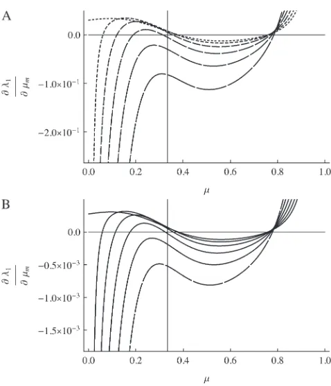
ð6Þ The stability of this point is determined by the eigenvalues ofL, which satisfy the equationM zð Þ ¼detðLzIÞ ¼0, Figure 1.—Comparison of @l₁=@m

m evaluated at mm ¼ mM ¼ m (solid curves) and @w*=@mM (shaded curves) for

n¼ 3. In all plots,s1 ¼101whereass3 ¼101, 100.8, and

100.6_{, in the top, middle, and bottom plots, respectively.}

where I is the 2 3 2 identity matrix. The positive eigenvalue ofLis,1 ifM(1).0 andM9(1).0 and is .1 ifM(1),0. In the former case,mcannot invade, while in the latter caseðx1*;0;x3*;0Þ is unstable andminvades. After a considerable amount of algebra we find the following.

Result 1. The equilibrium x*¼x1*;0;x3*;0 is stable

ifmm.mMand unstable ifmm,mM.For all recombination rates, a modifier allele that reduces the mutation rate will invade.

We can also show that the mean fitness w* at

x1*;0;x3*;0

is a decreasing function ofm_M.

This reduction principle in constant environments was proved for selection on diploids and any number of alleles at the mutation-controlling gene by Liberman and Feldman(1986).

CHANGING ENVIRONMENTS: INITIAL EQUILIBRIUM

Assume that in each generation the genotypic fit-nesses change. At generationi, fori¼1, 2,. . .,k, the fitness parameters are

gamete: AM Am aM am

fitness: wi₁ wi₁ wi₃ wi₃; ð7Þ

where again we assumeMandmdo not affect fitness. At the beginning of generationi, fori¼1, 2,. . .,k, the population state is given by the frequency vector

x¼ðx1;x2;x3;x4Þ, and at the beginning of generation

i11 it is given byx9¼x₁9;x9₂;x₃9;x9₄, wherex9¼Tið Þx

andTiis given by the system (1) with fitnesses (7):

wix9₁¼ ð1m_MÞwi₁ðx1rDÞ1mMwi3ðx31rDÞ

wix9₂¼ ð1m_mÞwi₁ðx21rDÞ1mmwi3ðx4rDÞ

wix9₃¼ ð1mMÞwi3ðx31rDÞ1mMwi1ðx1rDÞ

wix9₄¼ ð1mmÞwi3ðx4rDÞ1mmwi1ðx21rDÞ: ð8Þ The normalizing factor iswi_¼ðx11x2Þwi

11ðx31x4Þwi3

and the linkage disequilibrium isD¼x1x4x2x3. If the population state at the beginning of the k -generation process is xo _{¼ x}o

1;xo2;xo3;xo4

, then after generationkit isxk_{¼ x}k

1;xk2;xk3;xk4

wherexk_{¼T xð Þ}o

and the transformationT is given by the composition of thektransformations:

T ¼Tk+Tk1+ +T1: ð9Þ The combined mean fitness associated with the trans-formationTfromxo _toxk_is

w ¼wðxkÞ ¼Y k

i¼1

wiðxiÞ: ð10Þ

To study the evolution of mutation, we first consider a population where only the M allele is present at the modifier locus. LetSibe the transformation associated

withTirestricted to the two gametesAMandaMonly.

ThenSi, fori¼1, 2,. . .,k, is given by

wixi₁11 ¼ ð1m_MÞwi₁xi₁1m_Mwi₃xi₃

wixi311 ¼ ð1mMÞwi3xi31mMwi1xi1; ð11Þ withwi_{given by}

wi¼wi₁xi₁1wi₃x₃i; i¼1;2;. . .;k: ð12Þ The ‘‘total’’ k-generation transformation restricted to

AMandaMisS ¼Sk+Sk1+ +S1.

In (11) we can use the ratioui_¼xi

1=xi3 instead ofxi1

andxi

3, and similarlyui

11 _¼xi11 1 =xi

11

3 . Then the

trans-formationSiis

ui11¼fiðuiÞ ¼

ð1mMÞw1iui1mMwi3 mMwi1ui1ð1mMÞwi3

; i¼1;2;. . .;k:

ð13Þ Thus, the total k-generation transformation on the boundary where only Mis present is the composition

f ¼fk+fk1+ +f1.

Note that fiðÞis a linear fractional transformation.

One of the properties of such a transformation is that its composition overkgenerations is also a linear fractional transformation. Hence the totalk-generation transfor-mationfcan be written as

uk¼fðuÞ ¼au o_1b

cuo1d; ð14Þ

where, since the coefficients in (13) are positive for 0, mM,1, the coefficientsa,b,c, anddare also positive.

Now we can analyze the evolutionary process in terms of this k-generation transformation (14), and since it is linear fractional it converges to a unique stable equilib-rium. Thus, ultimately the population converges to a

k-step trajectory loop determined by the stable state of thisk-step compound linear fractional transformation. In fact,u*, the stable state of thek-step process, is the unique positive root of

QðuÞ ¼cu21ðdaÞub ¼0: ð15Þ Using the same notation as in Result 1, this equilibrium can be expressed as x*¼ðx1*;0;x3*;0Þ, and it can be shown to be globally stable.

CHANGING ENVIRONMENTS: EXTERNAL STABILITY

To explore the dynamics of switching, and in particular to find an evolutionarily stable switching rate (if it exists), we study the external stability of the unique internally stable equilibriumx* to invasion by the new mutation modifying allelem. The mutation ratemMproduced by allele M

will be evolutionarily stable if allele mcannot invade whenmm.mMormm,mM. Therefore we analyze the

external stability ofx* as a function of the difference between the new mutation rate mm and the resident

A population starting from the equilibrium x* sat-isfies x*¼T xð *Þ ¼Tk+Tk1+ +T1ðx*Þ; that is,

afterkgenerations of change it will end up again atx*. Takex¼x*1 eas a ‘‘starting’’ population state near

x*, where e¼ðe1;e2;e3;e4Þ with ei ‘‘small’’ and e11e21e31e4¼0 so thatx9¼T x¼x*1e9. We work

with the linear transformation ‘‘near’’x*; that is, up to nonlinear terms,

x9¼x*1e9¼x*1L*eT_{; ð16Þ}

where L* is a matrix that depends on x* and may be obtained as a combination of the matrices of similar linear approximations across the k generations. The stability of equilibriumx* to the introduction of allelem

is determined by the eigenvalues of the matrixL*. This scenario is well known from modifier theory (Feldman 1972; Feldman et al. 1980; Feldman and Liberman 1986), and the matrix L* is also known to have the structure

1 3 2 4

L*¼ Lin

* * * * 0 0 0 0 Lex

2 6 6 6 4 3 7 7 7 5 1 3 2 4

; ð17Þ

where we have swapped columns 2 and 3 and rows 2 and 3 to show the structure. The entries marked * do not affect the eigenvalues ofL*.

The eigenvalues of L are therefore those of the submatrices Lin and Lex, where Lin determines the

internal stability ofx*, confined to the boundary with onlyMpresent. Asx* is assumed to be stable there, these eigenvalues are less than one in magnitude.Lexis the

linear approximation of evolution near x*, which involves only the gametesAmandamand is a combina-tion of the matricesLex

i , fori¼1, 2,. . .,k, that describe

the changes in generationiwhen allelemis rare. In fact, from (8) we have

wi_Lex i

¼ ð1mmÞw

i

1r ð1mmÞwi1mmwi3

xi

3 mmwi31rð1mmÞwi1mmwi3

xi 1

mmwi11r ð1mmÞwi3mmwi1

xi

3 ð1mmÞwi3rð1mmÞwi3mmwi1

xi 1

" #

:

ð18Þ We setx*¼x1 _{and describe the following generations}

byx2_{;. . .;x}k_{. The normalizer in generationiis}

wi ¼wiðxiÞ ¼wi₁xi₁1wi₃xi₃: ð19Þ As each of the matricesLex

1 ;L ex 2 ;. . .;L

ex

k is positive,Lexis

also positive, and, by the Perron–Frobenius theory, the largest eigenvalue ofLexis positive. Some properties ofL

are documented insupporting information,File S1, Part I. The external stability of x* depends on the magni-tude of the positive, and largest, so-called Perron– Frobenius eigenvalue of Lex. If this eigenvalue is,1, x* is externally stable and allelemcannot invade near

x*, and if it is.1,x* is externally unstable, andmenters the population and increases in frequency.

The characteristic polynomial ofLex, namelyC(z)¼

det(Lex zI), is quadratic in z with a positive z2

coefficient. Therefore the largest positive eigenvalue ofLexis,1 whenC(1).0 andC9(1).0, and it is.1

when C(1) , 0. It seems impossible to computeC(1) and C9(1) in general. We are, however, able to derive analytical results in some special cases that are discussed in the following sections.

CYCLICALLY FLUCTUATING ENVIRONMENTS: PERIOD 2

Suppose that the selection regime alternates between two states as specified in (20) below.

genotype AM Am aM am

fitness regime 1 w1 w1 w3 w3 fitness regime 2 wˆ1 wˆ1 wˆ3 wˆ3:

ð20Þ

Environments alternate, producing a cycle with period 2. We first characterize the unique stable equilibrium

x*¼ðx1*;0;x3*;0Þ on the boundary where only M is present. On this boundary the two transformations S1

andS2of (11) are

S1/w 1_y

1 ¼ ð1mMÞw1x11mMw3x3

w1y3 ¼ ð1mMÞw3x31mMw1x1

ð21Þ

and

S2/w 2_x

19¼ ð1mMÞwˆ1y11mMwˆ3y3

w2x39¼ ð1mMÞwˆ3y31mMwˆ1y1

; ð22Þ

where x1 and x3 are the frequencies of AM and aM, respectively, at the beginning of generation 1,y1andy3

at the end of generation 1, andx91 andx93 at the end of generation 2. The mean fitnesses are

w1 ¼w1x11w3x3; w2¼wˆ1y11wˆ3y3: ð23Þ This cycle repeats with period 2, and the combined one-cycle transformationS¼S2+S1, on the boundary where Mis fixed, is

S/

w1w2x₁9¼ ð1m_MÞ2_w

1wˆ11m2Mw1wˆ3

x1 1m_Mð1m_MÞw3ðwˆ11wˆ3Þx3

w1w2x₃9¼ ð1m_MÞ2_w

3wˆ31m2Mw3wˆ1

x3 1m_Mð1m_MÞw1ðwˆ11wˆ3Þx1:

ð24Þ

The normalizing factorw¼w1_w2_{is thecycle mean fitness}

and can be expanded as

w¼ ½ð1mMÞ2w1wˆ11m2Mw1wˆ31mMð1mMÞw1ðwˆ11wˆ3Þx1

1½ð1mMÞ2w3wˆ31m2Mw3wˆ11mMð1mMÞw3ðwˆ11wˆ3Þx3

ð25Þ

¼wˆ1w1x11wˆ3w3x31mMðwˆ3wˆ1Þðw1x1w3x3Þ: ð26Þ

u9¼fðuÞ

¼ ð1mMÞ

2_w

1wˆ11m2Mw1wˆ3

u1mMð1mMÞw3ðwˆ11wˆ3Þ

mMð1mMÞw1ðwˆ11wˆ3Þu1 ð1mMÞ2w3wˆ31m2Mw3wˆ1

;

ð27Þ

whereu¼x1=x3andu9¼x9₁=x93.

The stable equilibrium x*¼ðx1*;0;x3*;0Þ with x1*¼ u*=ð11u*Þ and x3*¼1=ð11u*Þ satisfies u* ¼ u9 ¼ f(u*) and is the unique positive root of the quadratic equationQ(u)¼0, where

QðuÞ ¼mMð1mMÞw1ðwˆ11wˆ3Þu2

1 ð1mMÞ2ðw3wˆ3w1wˆ1Þ1m2Mðw3wˆ1w1wˆ3Þ

u

mMð1mMÞw3ðwˆ11wˆ3Þ: ð28Þ

We now check the external stability properties of x*, that is, its stability to invasion bymwhenmis introduced nearx*. Evolution of the mutation rate is determined by the external stability properties ofx*, that is, its stability to invasion bymwhenmis introduced nearx*. InFile S1we show thatmwill invade (i.e.,m_minvadesm_M) ifM(1),0, where

Mð1Þ ¼ðmmmMÞð1rÞD x*1

; ð29Þ

andD ¼D(r, mm) is shown inFile S2to be a bilinear

function ofrandmmin 0#r#1 and 0# mm#1.

In general it is very complicated to compute M(1), unless we assume that the fitnesses are symmetric; that is,

ˆ

w1¼w3 andw3ˆ ¼w1, which allows a complete analysis ofM(1) and the external stability ofx*. For generalr, mm, andmM, we refer to NumericalAnalysis, below. We

are able to obtain complete results when there is absolute linkage between the two loci (r¼0) andmm¼0 ormm¼1.

Whenr¼0, the matrixLex¼LˆL, withw* the product

ofw1_andw2_{at equilibrium, is given inFile S1, Part II by}

w*Lex¼ ð1mmÞ 2_w

1wˆ11m2mw1wˆ3 mmð1mmÞw3ðwˆ11wˆ3Þ

mmð1mmÞw1ðwˆ11wˆ3Þ ð1mmÞ2w3wˆ31m2mw3wˆ1

:

ð30Þ

When eithermm¼0 ormm¼1,Lexis a diagonal matrix,

and its eigenvalues are

l0₁¼w1wˆ1 w* ; l

0 2¼

w3wˆ3

w* formm¼0; l1₁¼w1wˆ3

w* ; l 1 2¼

w3wˆ1

w* formm¼1: ð31Þ

The magnitude of the leading eigenvalue depends on the asymmetry of the parameters w1ˆ andw3ˆ , with respect tow1andw3. This asymmetry may be represen-ted by the parameter

d¼w3wˆ3w1wˆ1: ð32Þ As the fitnesses are relative, and hence determined up to a multiplicative positive constant in each generation,

d ¼0 implies that w3ˆ ¼w1andw1ˆ ¼w3, namely

com-plete symmetry between the two allelesAanda, whereas d6¼0 implies asymmetry.

Whend¼0 (i.e., the symmetric casew3ˆ ¼w1;w1ˆ ¼ w3 discussed in the next section), it turns out thatl0 1

andl0

2are,1, whereas at least one of the eigenvalues

l1 1andl

1

2is.1. Therefore whenmm¼0,x* is externally

stable for all 0,mM#1, and whenmm¼1,x* is never

stable when 0# mM,1. Thus whenr¼0, a

mutation-reducing allele cannot invade. The results are sensitive to the asymmetry measured, as is discussed in greater detail later.

THE SYMMETRIC CASE WITH PERIOD 2

In the symmetric case where the selection regime alternates each generation, we have w1ˆ ¼w3;w3ˆ ¼ w1 ðd¼w3w3ˆ w1w1ˆ ¼0Þ, and we can present a

com-plete external stability analysis of the equilibriumx*. In the symmetric case, the fitness parameters fluctuate between generations such that

genotype AM Am aM am

odd generation fitness w1 w1 w3 w3 even generation fitness w3 w3 w1 w1

; ð33Þ

where, of course, we assume w1 6¼ w3. The unique internally stable equilibrium x*¼ðx1*; 0; x3*; 0Þ on the boundary where only allele M is present can be represented as x1*¼u*=ð11u*Þ, x*

3 ¼1=ð11u*Þ,

where u* is the unique positive root of the quadratic Equation 15, which becomes

QðuÞ ¼ ð1mMÞw1u21mMðw3w1Þu ð1mMÞw3¼0: ð34Þ

InFile S3we use (34) to analyze the factors in (29). From (29),M(1)¼0 whenr¼1, in which case the larger eigenvalue is 1. When 0 # r , 1, the sign of M (1) depends on the signs of (mmmM) and the sign ofD¼

D (r, mm). In fact we show in File S3 that the bilinear

function D(r,m_m) is always negative in the symmetric case. As an immediate consequence of this, together with the representation ofM(1) given in (29), we secure the following result.

Result 2.The internally stable equilibrium is externally

stable whenmM.mmand is unstable whenmM,mmfor all

0 # r , 1. Thus with symmetric changing environments,

higher mutation rates are favored.

As in the case of constant environments, Result 2 accords with the behavior of the mean fitness at equilibrium as a function of the resident mutation rate. With symmetric changing environments we can show the following.

Result3.The mean fitness w*¼w*(m_M)at equilibrium is

The proof of this result can be found inFile S4.

THE SYMMETRIC CASE WITH PERIOD 4

The fitnesses of the genotypes can be represented as follows:

genotype AM Am aM am

generation 1 w1 w1 w3 w3 generation 2 w1 w1 w3 w3 generation 3 w3 w3 w1 w1 generation 4 w3 w3 w1 w1:

ð35Þ

In this case, on the boundary where Mis fixed, the four-generation recursion is

wx9¼T2+T2+T1+T1ðxÞ; ð36Þ where, as in (21) and (22),

T1¼

ð1m_MÞw1 mMw3 mMw1 ð1mMÞw3

;

T2¼

ð1mMÞw3 mMw1 m_Mw3 ð1mMÞw1

; ð37Þ

and the four-generation normalization factor is then

w¼w2₁w2₃1m_Mð1m_MÞw1w3ðw1w3Þ2

1m_Mð1m_MÞðw11w3Þ2ðw1w3Þðw1x1w3x3Þ: ð38Þ

Our argument proceeds in much the same way as for the symmetric model with period 2. First we show inFile S5, Part I that whenr¼0,

ðw1w3Þðw1x1*w3x3*Þ.0; ð39Þ where x1*;x3* _{denotes the equilibrium of the} four-generation transformation. Hence, from (38)

w$w2₁w2₃: ð40Þ

We now turn to the external stability ofx1*;0;x3*;0, which is determined by the eigenvalues ofLex. When

mM¼0, we can write

w*Lex¼

w3 0 0 w1

2

w1 0 0 w3

2

¼ w21w23 0 0 w2₁w2₃

;

ð41Þ

and whenmM¼1,

w*Lex¼ 0 w1

w3 0

2

0 w3

w1 0

2

¼ w21w23 0 0 w2₁w2₃

:

ð42Þ

But by (40),w*.w2 1w

2

3, and thereforex* is externally

stable when eitherm_M¼0 orm_M¼1. In other words, if

0 , mM , 1, then a new mutation-modifying allele

cannot invadex* if it produces mutation rates that are too high or too low. This leaves open the possibility that there might be an intermediate value of the mutation rate mMthat gives rise to an equilibriumx* on theM

-fixed boundary that cannot be invaded. The first indication thatmM ¼1₂ is this value is suggested by the

following.

Result4. In the period 4 symmetric case,if r¼0,the mean

fitness w*¼w*(m_M)achieves a maximum atm_M ¼1 2. The proof is inFile S5, Part II.

If m_M ¼1

2, then the single-generation transforma-tions are very symmetric, and the equilibrium on the

M-fixed boundary has x1*¼1

2 ¼x3*. To examine the invasion bymm6¼1₂ we evaluate the external stability of x*¼ 1

2; 0; 12; 0

. The eigenvalues of the linear ap-proximation Lex near x* are the roots ofM (z) ¼0,

whereM(z) can be expressed as

MðzÞ ¼ ðw*zÞ2 _{ðw*zÞðA1DÞ1ADBC; ð43Þ} where the entries ofLex,A,B,C,Dare all positive. As

before, one eigenvalue is positive, and it can be shown that detLex¼ADBC ¼ð12mmÞ

4 w4

1w 4

3.0. Hence

both eigenvalues are positive. The larger one is ,1 if

M(1).0, which is shown to be the case inFile S5, Parts III and IV. This allows us to claim the following.

Result5.In the period4symmetric case with0#r#1,the

mutation rate mM ¼1₂ cannot be invaded by mutation rates either.or,1

2.

For cycles of periodm¼2n, whenr¼0, we can show that if 0 , mM# 1, a modifier allelemthat produces

mm ¼0 cannot invade. Ifn is even we are also able to

prove that allelemwithmm¼1 cannot invade. It remains

to prove the latter result for odd values ofn, and we see innumerical analysisthat this could be difficult.

THE MEAN FITNESS AND EIGENVALUE CRITERIA

The analyses by Ishii et al. (1989) and Gaa´ l _{et al.} (2010) formulated the dynamics of M and m, the mutation-controlling alleles, in terms of the numbers of each genotype. In particular, whenr¼0, Ishiiet al. concluded that the criterion for invasion and long-term increase of m in a population monomorphic for M

mutation, and migration also maximized the mean fitness.

Our criterion for initial increase is in terms of the local stability of the equilibriumx1*;0;x3*;_{0, wherex1*}

and x3* are functions of mM, to invasion by m. This

invasion is determined by the leading eigenvaluel of the local stability matrix that gives the frequencies ofAm

andamnearx1*;0;x3*;0_{, and}lmust be a function of both mm and mM. As pointed out above, the relevant

properties of l are expressible in terms of properties of M(l), the characteristic polynomial of the local stability matrix Lex. The value of mm that makes

@l=@m_mjmm¼mM ¼0 will be the stable value of the

muta-tion rate.

We write the local stability matrix for local dynamics of

Am,amnearx1*;0;x3*;0_as

˜ A w* ˜ B w* ˜ C w* ˜ D w* " #

; ð44Þ

where the entriesA˜;B˜;C˜;D˜ are defined by the contin-ued operation of the linear fractional transformation corresponding toLex,w* is a function ofmM, and the

tilde indicates that the numerators of all entries are functions ofmm. We can write the characteristic

poly-nomialM(l) of matrix (44) as

MðlÞ ¼ ðlw*Þ2 _ðl

w*Þð_A˜1_D˜Þ1A ˜˜D_{B ˜}˜_C: ð45Þ

From (45) we can calculate@l/@m_m.

For the initial equilibriumx1*;0;x3*;0_{, where allele}

mis absent, we have

x*1

x*3

! ¼ ˆ A w* ˆ B w* ˆ C w* ˆ D w* " # x*1

x*3

!

; ð46Þ

where the circumflex indicates that the numerators are functions ofmM. From (46), the matrix has an

eigen-value of 1, and we have

ðw*Þ2_{w*ðAˆ1DˆÞ1ðA ˆˆDB ˆˆCÞ ¼0: ð47Þ}

The stationary values ofw* with respect tom_Mcan be obtained by differentiating Equation 47 with respect to mM and finding values ofmMsuch that @w*/@mM ¼0.

The relationship between mutation values, which max-imize the mean fitness, and the uninvadable value ofm that sets@l=@mmjmm¼mM ¼0 is given by the following.

Result6.Mutation ratesm_Mthat are critical points of the

mean fitness w*in the case r¼0also entail that atmm¼mM,

@l/@mm¼0.

The proof is in theappendix. Figure 1 plots@w*/@m_M and@l/@mmforn¼3, and the two derivatives are seen

to vanish at the same value of the mutation rate. The proof of Result 6 actually makes no use of the symmetry

of the fitnesses, so Result 6 is also true for asymmetric fitnesses.

NUMERICAL ANALYSIS

Result 2 entails that in the symmetric case d¼ w3w3ˆ w1w1ˆ ¼0, for period 2 (n¼1) for all values of

the recombination rate, nonzero values of the resident mutation ratemMwill be invaded by allelemthat gives

rise to a higher mutation rate; i.e., mm . mM. The

mutation rate will therefore go on increasing to its maximum of 1. A similar result for period 4 (n ¼2), namely Result 5, tells us that for allr, values ofm_M,1 2 will be invaded by higher valuesm_m.m_M, but values of m_M.1

2 will be invaded by lower values ofmm. There are no constraints on the strength of the symmetric selec-tion as were required in the analysis by Ishiiet al. (1989). There have been suggestions in the literature that the stability of the mutation ratem¼1/nfor the symmetric model cycles with period 2n holds for larger values ofn(Ishiiet al.1989; Lachmannand Jablonka1996). For the asymmetric model, with d 6¼ 0, however, Salathe´ et al. (2009) showed that the situation was much more complicated and that if the asymmetry was large enough, zero was the stable mutation rate; mutation provided no advantage with fixed or random period cycles. Further, with stochastic environments and a rate of environmental change of 1/nevery generation, the stable switching rate can be up to two orders of magnitude lower than 1/n(Salathe´ _{et al.}2009, Figure 1). In addition, we noted after Result 5 above that even in the caser¼0, ifnis odd there may be some anomalies. We have therefore explored three effects numerically: the role ofnand in particular whether it is odd or even, the role of asymmetry in the cycling fitness values (extending Salathe´ et al. 2009), and the effect of recombination between the major locus and the muta-tion modifier. The equilibrium _ðx1*;0;x3*;_{0Þ is found}

numerically and for given parameter values, the matrix Lexis determined numerically together with its

eigen-values. The leading eigenvaluel1is numerically

differ-entiated with respect tom_mand the derivative evaluated atm_M¼m_m, where as we showed in (29) the eigenvalue is 1. The sign of @l₁=@m_mjmM¼mm then tells us whether a

larger or smaller value ofm_m will producel1. 1 and

hence cause mto invade. Thus, points where @l1/@m crosses zero with a negative slope indicate values ofmM

that cannot be invaded by any nearby value ofmm. These

values of mMcan be regarded as evolutionarily stable.

These results are summarized in Figure 2.

allr. In what follows, we use the notationwð Þ1i ¼1s1; wð Þ3i ¼1 forngenerations withw

i ð Þ 1 ¼1;w

i ð Þ

3 ¼1s3for

the next n generations. Thus, s1 ¼ s3 corresponds to perfect symmetry in selection regimes (Salathe´ et al. 2009). Note that in all graphs withr¼0 and in many of the others, there is an interval of asymmetry in the selection coefficients s1¼ 1w1and s3¼ 1w3in which there is a stable nonzero mutation rate. Asnandr

increase, the stable nonzero mutation rate withs1¼s3

decreases. For r¼0 and smalls1ands3, the extent of asymmetry that allows a stable nonzero mutation rate does not change much with n, whereas for the r . 0 values shown in Figure 2 it is very sensitive ton.

To ascertain that the existence of a range of asymme-try permitting a stable nonzero mutation rate was not an artifact of the numerical procedure, forr¼0 then¼2 andn¼3 cases were repeated using a very accurate nu-merical derivative [complex step derivative (Squireand Trapp1998)] and a finer array ofs3values fors1¼0.01 ands1¼0.1. Then ¼2 results are in Figure 3 where there can be no doubt that this band of asymmetric fitnesses allowing a stable mutation rate at or very close to1₂ really exists. We see that in Figure 3, A and B,@l1/

@mis positive form,1

2 and negative form.12 whens1¼s3 and thatm-values near1

2 are stable for a range ofm-values that decreases as the asymmetry increases, with m¼0 becoming stable when the asymmetry is too great. The width of the band of stability is a little,1 log10fitness

unit in both Figures 3 and 4. Figure 4 shows the same effect forn¼3. In Figure 4, A and B,@l1/@mm¼0 occurs

close tom_m¼1

3, but not exactly at 1

3, which would be the case if 1/nwere the evolutionarily stable mutation rate. Figures 5 and 6 offer another view of the stability/ invasibility parameter ranges. Figure 5 sets r¼0 while

r¼0.3 in Figure 6. In these figures, the solid areas have the leading eigenvalue ,1, while it is.1 in the open regions. In the first row of both figures we see first the stability of m¼1

2, and as s3 increases the black area under the separating diagonal reflects the range of stable mutation rates near1

2, which disappears whens1¼ 0.01 ands1¼0.03, leaving zero as the stable mutation rate. In general, we see that whens3is different froms1, an unstable equilibrium inmappears below the stable equilibrium. If the mutation changes in sufficiently small steps, thenmcan be trapped below the unstable equilib-rium and evolve to 0. As long as the rate may take larger Figure2.—Evolutionarily stable

mu-tation rates as a function of the selec-tion coefficients for the disfavored allele in each environment, s1 ¼ 1

w1ands3¼1w3, which are plotted

steps, and if the rate remains below1

2, it will eventually converge to the stable equilibrium. Ass3increases further, the stable and unstable equilibria annihilate one another andmgoes to 0, if it remains below1

2.

Withnodd, the complication alluded to after Result 5 becomes visible: the first columns of Figures 5 and 6 show the symmetric model, and the second and fourth rows are examples withnodd. Withn¼3 we see a stable value of the mutation rate,1₂ and near1₃. In general, whennis odd, andr¼0, an unstable equilibrium value ofmappears withm.1

2. Thus, larger values ofm may also be invadable by even larger values, depending on the difference between the resident m_M and the in-vadingm_m. The domains of attraction in the asymmetric cases can become very complicated; compares3¼0.015,

n¼3, andr¼0 withr¼0.3. Note that withn¼20 and 21,r¼0.3 forces stability ofm¼0 for most cases, while withr¼0,s3¼0.015, andn¼21, there is a range of high mutation rates that will be invaded by even higher (although unrealistic) mutation rates. Examination of Figures 5 and 6 suggests that if both mutation ratesmM

andmm are very small, odd and even values of n give

qualitatively similar results. For values ofmMandmm,

1

2, the patterns forn¼2 andn¼3 are similar for both

r¼0 andr¼0.3. In the unrealistic range of mutation rates .0.5, n ¼ 2 and n ¼3 show different patterns

of invasibility with m ¼1 stable forn ¼3 but not for

n¼2.

For large values ofs1ands3the range of asymmetry that allows a stable nonzero mutation rate increases asn

increases, but for given n, it decreases as r increases. Note that for larger recombination rates and largern, the stable mutation rates, if different from 0, are>1/n. Comparing the effect of recombination whennis small with that when nis large, we have an indication from Figure 5 (r¼0) and Figure 6 (r¼0.3) that increasing recombination makes it more likely that the mutation rate will decrease.

Salathe´ et al. (2009) showed for the symmetric selection case that if the period of the cycle was a gamma-distributed random variable, the stable switch-ing rate dropped precipitously as the variance in the cycle period increased, compared to the case where the period was fixed at the mean of the gamma distribution. Figure 7 illustrates the interaction between recombina-tion and variance in the cycle period. The effect of recombination on the evolutionarily stable mutation rate is striking: withr¼0.2, for example (second panel from the right in Figure 7), none of the mutation rates near 1/nthat are stable when the period is fixed at 2n

(red–pink in the leftmost panel) are stable. Moving from left to right in Figure 7, recombination is seen to strengthen the effect of randomness in the period seen by Salathe´ et al.(2009, Figure 1) in shifting the stable mutation rate to substantially,1/n. It is reasonable to expect that with asymmetries in fitness, recombination would also enhance the tendency of variance in the Figure3.—Plot of the derivative of the leading eigenvalue,

l1, with respect tommevaluated atmM¼mm¼mwhenn¼2

andr¼0. (A)s1¼1w1¼101and the lines from shortest

dashes to longest dashes ares3¼1w3¼101, 100.9, 100.8,

100.7_{, 10}0.6_{, and 10}0.5_{. (B)s}

1¼0.01 and the lines from

short-est dashes to longshort-est dashes ares3¼102, 101.9, 101.8, 101.7,

101.6_{, and 10}1.5_{. The vertical line is located atm¼1/n¼}1 2.

Figure4.—(A and B) The same as Figure 3, exceptn¼3.

cycle period to decrease the evolutionarily stable rate of phenotypic switching.

DISCUSSION

The contribution of epigenetic phenomena to both statistical and dynamic properties of phenotypic varia-tion has received much recent attenvaria-tion. In general, the two aspects, statistical and dynamic, have been well separated. The statistical treatment by Slatkin(2009) quantifies the contribution of epigenetic change to disease risk, where the epigenetic effect could be mutational and act on gene expression. Another recent analysis by Danchin and Wagner (2010) introduces transmitted epigenetic variance as well as ‘‘culture’’ through transmitted social variance into calculations of heritability; addition of these effect leads them to ‘‘inclusive heritability,’’ which they define as all in-herited components of phenotypic variance. Their framework is a special case of early work on the contributions of cultural inheritance to estimated her-itability by Cavalli-Sforzaand Feldman (1978) and Feldmanand Cavalli-Sforza(1979) that predates the current interest in cultural inheritance as a possible cause of transgenerational epigenetics.

Such statistical treatments usually do not include recombination as a force that affects the genetic or epi-genetic contributions to phenotypic variance. For

ex-ample, multilocus evolutionary simulation studies by Feinbergand Irizarry(2010) of epigenetic variation were stimulated by findings of dietary modification of DNA methylation of theAgoutigene in mice and meth-ylation of the Axin-fused allele in kinked-tail mice (Cooney et al. 2002; Rakyan et al.2003; Waterland and Jirtle 2003). Recombination was not included in the simulations by Feinberg and Irizarry.

Studies motivated by the adjustment by microorgan-isms of their gene regulation to environmental change, such as those mentioned in the Introduction, ignore recombination because it is assumed to be rare in the bacteria, yeast, or cellular populations on which the models are based. As a general rule, these models take populations of cells that do not compete and compare their exponential growth dynamics under different conditions. Thus, the recent study by Leibler and Kussell (2010) focused on the historical phenotypic states of a population of nonrecombining cells, and fitness in different populations was measured as a property of these histories. Recombination would be difficult to include in such a treatment for the same reason that coalescent analysis in genetics is compli-cated by recombination and selection. Similarly Gerland and Hwa(2009) measure the success in populations of cells subject to mutation by the genetic load, namely the reduction below the maximum fitness possible caused by deleterious mutations in a single population. Here Figure5.—Pairwise invasibility plots

for mutation rate modifier. Combina-tions of resident mutation rate mM

and invading mutation rate mm in the

open regions yield a leading eigenvalue .1 in absolute magnitude; the leading eigenvalue is ,1 in the solid regions. We assume thatw1¼1 s1and w3 ¼

1s3and sets1¼0.01. Each row denotes

a different value for n, the number of generations in each environment. The recombination rate is set tor¼0. Note that thex- andy-axes are logarithmically scaled from 102 _{to 0.5 and from 1}

again the analysis is in terms of a single gene, and re-combination does not enter into the dynamics of the different mutational states. However, Lynch (2007, p. 89) points out that ‘‘recombination at the nucleotide level does not appear to be exceptionally low in pro-karyotes when compared to that in multicellular species.’’ Inclusion of recombination between the locus under selection and the locus that controls the mutation rate is important but greatly increases the difficulty of exact analysis when the selection fluctuates over time. For-mally the reason for this is that atr¼0 the recursion system is linear fractional, and iterates of linear frac-tional transformations remain linear fracfrac-tional, even if the parameters are not constant over time. In particular, this guarantees that we can model the starting point of the modification process as the unique stable trajectory of the compound linear fractional system. The initial dynamics of the rare mutation-modifying allele can then be analyzed as in Libermanand Feldman(1986). The argument makes use of the positivity of the initial increase matrix specified by Lex (Equations 17–19).

Whenr.0, the linear fractional structure is replaced by a much more complicated dynamical iteration whose properties are difficult to discern in general. With suf-ficiently weak selection and small values ofjm_M m_mj, however, M’Gonigle et al. (2009) made considerable progress in the case where cycling was due to host– parasite interactions.

Our analysis of the symmetric cases withn¼1 and 2, corresponding to periods 2 and 4, respectively, for the fitness cycle, confirms results found numerically by Ishii

et al. (1989). They were able to study the system an-alytically in these cases under one of two restrictive conditions: the weak selection limit s>1=n (where, in our terminology,s1¼1w1, for example, as in Figures 1 through 7) or s1 close to 1 (which entails in our terminology that 1w10). Our Results 3 and 5 and the proofs inFile S1,File S2,File S3,File S4, andFile S5 show analytically thatm¼1 andm¼1

2 are the uninvad-able mutation rates forn¼1 andn ¼2, respectively, with no restrictions on the recombination rate or fitnessesw1andw3.

As pointed out by Ishiiet al.(1989), odd values ofn produce two equilibria for the mutation rate, a stable value ,0.5 and an unstable one .0.5. As n becomes larger, however, our Figures 5 and 6, with n¼21 and symmetric fitnesses show that increasingrcan eliminate the large unstable value ofm; withr ¼0.3, in the first column of Figure 6, the value ofm,1

2 is stable from abovem, while in Figure 5, where r ¼0, m¼ 1 has a domain of stability above the unstable equilibrium.

In both symmetric casesn¼1 andn¼2, we proved that the mutation rates that cannot be invaded by any other (m¼1 forn¼1 andm¼1

2 forn¼2) are also the mutation rates that maximize the mean fitness w*. Those studies (e.g., Ishiiet al. 1989; Gaa´ l_{et al.} 2010)

Figure 6.—The same as Figure 5

that argue in terms of long-term growth rates in exponentially growing populations find that this is true for anyn. Our Result 5 provides an elegant resolution of the difference, with symmetric or asymmetric fitnesses andr¼0: the value ofmwhere@l/@mvanishes, namely the value that gives ‘‘eigenvalue stability,’’ is the same value that maximizes the logarithm of the long-term mean fitness, namely ðw*Þ1ð@w*=@m_MÞ. Numerical analysis confirms thatðw*Þ1

is indeed the factor that relates these derivatives, and the proof is given in the appendix.

Our analysis of symmetric selection shows some degree of robustness. From Figure 2 (and also Figures 3 and 4), there is a band of mildly asymmetric fitnesses surrounding the symmetric selection valuess1¼1w1¼ s3¼1w3in which the stable mutation rate is very close indeed to that obtained under symmetric fitnesses. For large values of boths1ands3this band becomes wider as

n increases for all recombination values (top right of each panel in Figure 2). For weaker asymmetric selec-tion this band narrows substantially, and the stable mutation rate becomes smaller as the recombination rate increases. Thus, asr increases, a greater range of

fitness asymmetries leads to a stable mutation rate of zero, except forn¼2. Even forn¼3 in the symmetric case, however, Figure 4 shows clear distance between the stable values ofmand the value1

3 predicted,e.g., by Ishii

et al.(1989) and Lachmannand Jablonka(1996). At

n¼100, in Figure 2, the stablemin the symmetric case is much closer to 2

100 than to1001 . Asrincreases, the stable value ofmin the symmetric case rapidly decreases below 1/n, and the band of stable nonzero mutation rates disappears. These results suggest that the optimal rate of phenotypic switching depends as much on the strength of selection in each environment as it does on the frequency of environmental changes, represented here byn; Kussellet al.(2005) claimed thatnwas much more important than the magnitudes of s1 and s3 in deter-mining the uninvadablem. At least for the values ofnwe tried, Figures 2, 5, and 6 show thats1ands3are indeed important.

Our earlier numerical study (Salathe´ et al. 2009) showed that in asymmetric fitness landscapes (w16¼w3), stable nonzero mutation rates required very strong selection in both environments (i.e., large s1 and s3). Our Figures 5 and 6 show an interesting feature of the dynamical system that distinguishes odd and even values ofn. The numerical analysis illustrates that there may be more than one solution to@l=@m_mjmm¼mM ¼0 and that

the direction of selection on m_m might depend deli-cately on the sign and magnitude of (m_Mm_m). Why this is more likely to happen whennis odd than whennis even remains an interesting mathematical question. In both Figures 5 and 6,i.e., recombinationr¼0.0 and 0.3, forn¼3, there are three critical values ofmwhens1¼ 0.01 and s3 ¼ 0.015 and 0.02; one value is .0.5 and unstable, and two values are,0.5, with the greater of these locally stable, while the smaller one is locally unstable. The same pattern is exhibited forn¼21 with

r¼0 (Figure 5), but not forr¼0.3 (Figure 6). Figures 2 and 7 suggest that increasing recombination makes it less likely that a stable nonzero mutation rate will exist with either a fixed or a random switching period (see also M’Gonigleet al.2009). This suggests that switching in sexual organisms is less likely than in asexuals, and that if it occurs by genetic regulation of gene expression, the regulators should be linked to the genes they regulate. The role of recombination becomes more important as the period becomes longer, especially in symmetric or weakly asymmetric selection regimes.

The authors thank Freddy Christiansen for his careful reading of an earlier draft and two anonymous referees for incisive and useful comments. This research was supported in part by National Institutes of Health grant GM 28016.

LITERATURE CITED

Acar_{, M., J. T. M}ettetal _{and A.} van_Oudenaarden_{, 2008}

Sto-chastic switching as a survival strategy in fluctuating environ-ments. Nat. Genet.40:471–475.

Figure7.—Simulated evolutionarily stable mutation rates

withw1¼ w3 ¼1s. The numbers of generations in each

environment are drawn from a gamma distribution with mean 20 and variances2_{. Each panel denotes a different value of the}

recombination rate given in the first row. Colors denote the stable mutation rate, as in Figure 2. Each stable rate is the av-erage of 100 simulations; each simulation consists of iterating the recursion system (8) to determine whether a new ratemm

can invade an old ratemM. One thousand successive new rates

Balaban, N. Q., J. Merrin, R. Chait, L. Kowalikand S. Leibler,

2004 Bacterial persistence as a phenotypic switch. Science305: 1622–1625.

Bergman_{, A., and M. W. F}eldman_{, 1990 More on selection for and}

against recombination. Theor. Popul. Biol.38:68–92.

Bonduriansky_{, R., and T. D}ay_{, 2009 Nongenetic inheritance and}

its evolutionary implications. Annu. Rev. Ecol. Syst.40:103–125. Cavalli-Sforza, L. L., and M. W. Feldman, 1978 The evolution of

continuous variation. III. Joint transmission of genotype, pheno-type and environment. Genetics90:391–425.

Charlesworth_{, B., 1976 Recombination modification in a}

fluctu-ating environment. Genetics83:181–195.

Cooney_{, C. A., A. A. D}ave_{and G. L. W}olff_{, 2002 Maternal methyl}

supplements in mice affect epigenetic variation and DNA methy-lation of offspring. J. Nutr.132(Suppl. 8): 23935–24005. Danchin, E., and R. H. Wagner, 2010 Inclusive heritability:

com-bining genetic and nongenetic information to study animal cul-ture. Oikos119:210–218.

Feinberg, A. P., and R. A. Irizarry, 2010 Stochastic epigenetic

variation as a driving force of development, evolutionary adap-tation, and disease. Proc. Natl. Acad. Sci. USA107(Suppl. 1): 1757–1764.

Feldman, M. W., 1972 Selection for linkage modification: I.

Ran-dom mating populations. Theor. Popul. Biol.3:324–346. Feldman, M. W., and L. L. Cavalli-Sforza, 1979 Aspects of

vari-ance and covarivari-ance analysis with cultural inheritvari-ance. Theor. Popul. Biol.15:276–307.

Feldman, M. W., and U. Liberman, 1986 An evolutionary reduction

principle for genetic modifiers. Proc. Natl. Acad. Sci. USA83: 4824–4827.

Feldman_{, M. W., F. B. C}hristiansen _{and L. D. B}rooks_,

1980 Evolution of recombination in a constant environment. Proc. Natl. Acad. Sci. USA77:4838–4841.

Feldman, M. W., S. P. Ottoand F. B. Christiansen, 1997 Population

genetic perspectives on the evolution of recombination. Annu. Rev. Genet.30:261–295.

Gaa´ l_{, B., J. W. P}itchford_{and A. J. W}ood_{, 2010 Exact results for the}

evolution of stochastic switching in variable asymmetric environ-ments. Genetics184:1113–1119.

Gandon_{, S., and S. P. O}tto_{, 2007 The evolution of sex and}

recom-bination in response to abiotic or coevolutionary fluctuations in epistasis. Genetics175:1835–1853.

Gerland, U., and T. Hwa, 2009 Evolutionary selection between

al-ternative modes of gene regulation. Proc. Natl. Acad. Sci. USA 106:8841–8846.

Hamilton_{, W. D., 1980 Sex versus non-sex versus parasite. Oikos35:}

282–290.

Haraguchi, Y., and A. Sasaki, 1996 Host-parasite arms race in

mu-tation modifications: indefinite escalation despite a heavy load? J. Theor. Biol.183:121–137.

Henderson_{, I. R., and S. E. J}acobsen_{, 2007 Epigenetic inheritance}

in plants. Nature447:418–424.

Ishii_{, K., H. M}atsuda_{, Y. I}wasa_{and A. S}asaki_{, 1989 Evolutionary}

stable mutation rate in a periodically changing environment. Genetics121:163–174.

Karlin, S., and J. L. McGregor, 1972 The evolutionary development

of modifier genes. Proc. Natl. Acad. Sci. USA69:3611–3614.

Karlin, S., and J. L. McGregor, 1974 Towards a theory of the

evo-lution of modifier genes. Theor. Popul. Biol.5:59–105. Kussell, E., and S. Leibler, 2005 Phenotypic diversity, population

growth, and information in fluctuating environments. Science 309:2075–2078.

Kussell_{, E., R. K}ishony_{and N. Q. B}alaban_{, 2005 Bacterial}

persis-tence: a model of survival in changing environments. Genetics 169:1807–1814.

Lachmann_{, M., and E. J}ablonka_{, 1996 The inheritance of}

pheno-types: an adaptation to fluctuating environments. J. Theor. Biol. 181:1–9.

Leibler, S., and E. Kussell, 2010 Individual histories and selection

in heterogeneous populations. Proc. Natl. Acad. Sci. USA107: 13183–13188.

Liberman_{, U., and M. W. F}eldman_{, 1986 Modifiers of mutation}

rate: a general reduction principle. Theor. Popul. Biol. 30: 125–142.

Lim, H. N., and A.vanOudenaarden, 2007 A multistep epigenetic

switch enables the stable inheritance of DNA methylation states. Nat. Genet.39:269–275.

Lynch, M., 2007 The Origins of Genome Architecture.Sinauer

Associ-ates, Sunderland, MA.

MaynardSmith, J., 1978 The Evolution of Sex.Cambridge University

Press, Cambridge, UK.

Maynard Smith, J., 1980 Selection for recombination in a

poly-genic model. Genet. Res.35:269–277.

Maynard Smith, J., 1988 Selection for recombination in a

poly-genic model—the mechanism. Genet. Res.51:59–63.

M’Gonigle_{, L. K., J. J. S}hen_{and S. P. O}tto_{, 2009 Mutating away}

from your enemies: the evolution of mutation rate in a host-parasite system. Theor. Popul. Biol.75:301–311.

Nee, S., 1989 Antagonistic co-evolution and evolution of genotypic

randomization. J. Theor. Biol.140:499–518.

Rakyan, V. K., S. Chong, M. E. Champ, P. C. Cuthbert, H. D.

Morgan_{et al., 2003 Transgenerational inheritance of}

epige-netic states at the murineAxinFu_{allele occurs after maternal}

and paternal transmission. Proc. Natl. Acad. Sci. USA 100: 2538–2543.

Salathe´, M., J. VanCleveand M. W. Feldman, 2009 Evolution

of stochastic switching rates in asymmetric fitness landscapes. Genetics182:1159–1164.

Slatkin_{, M., 2009 Epigenetic inheritance and the missing}

heritabil-ity problem. Genetics182:845–850.

Squire_{, W., and G. T}rapp_{, 1998 Using complex variables to estimate}

derivatives of real functions. SIAM Rev.40:110–112.

Thattai_{, M., and A.}van_Oudenaarden_{, 2004 Stochastic gene}

expression in fluctuating environments. Genetics167:523– 530.

Waterland_{, R. A., and R. I. J}irtle_{, 2003 Transposable elements:}

targets for early nutritional effects on epigenetic gene regulation. Mol. Biol. Evol.23:5293–5300.

Youngson, N. A., and E. Whitelaw, 2008 Transgenerational

epige-netic effects. Annu. Rev. Genet. Hum. Genet.9:233–257.

APPENDIX

Proof that@w*=@mM ¼0 if and only if@l=@mmjmm¼mM ¼0.

From (45) we have atl¼1,

2@l

@m_mðw*Þ 2 @l

@m_mw*ðA˜1D˜Þ w*

@ð_A˜1D˜Þ

@m_m 1

@ð_{A ˜}˜_{DB ˜}˜_CÞ

@m_m ¼0; ðA1Þ

which we can reorganize atmm¼mMas

w* 2 @l

@mm

w* @l

@mm

ð_A˜1_D˜_Þ

mm¼m_M

¼w*@ðA˜1D˜Þ

@mm

mm¼m_M

@ðA ˜˜DB ˜˜CÞ

@mm

mm¼m_M

; ðA2Þ

or

@l

@m_m

_m

m¼m_M

¼w*ð@ðA˜1D˜Þ=@mmÞ @ðA ˜˜DB ˜˜CÞ=@mm w* 2½ w* ð_A˜1_D˜Þ

_m

m¼m_M

: ðA3Þ

But, from Equation 47,

@w*

@mM

¼w*ð@ðAˆ1DˆÞ=@mMÞ @ðA ˆˆDB ˆˆCÞ=@mM

2w* ðAˆ1_Dˆ_Þ : ðA4Þ

SinceA˜;B˜;C˜;D˜ are exactly the same asAˆ;Bˆ;Cˆ;Dˆ withmmreplacingmM, we conclude that

@l

@m_m

_m

m¼m_M

¼@w*=@mM

w* ¼

@logw*

@m_M : ðA5Þ

GENETICS

Supporting Information

http://www.genetics.org/cgi/content/full/genetics.110.123620/DC1

On the Evolution of Mutation in Changing Environments:

Recombination and Phenotypic Switching

Uri Liberman, Jeremy Van Cleve and Marcus W. Feldman

Liberman et al. 1 SI

FILE S1

Part I: Some general properties of the transformation

L

L

L

We can gain some insight into the eigenvalues of

L

L

L

by the following observations.

Observation I

(i)

det(

L

L

L

ex_i

) =

(1

−

2µ

m

)(1

−

r)w

i

1

w

3i

(w

i

₎

2

(A1)

(ii)

det(

L

L

L

ex) =

(1

−

2µ

m

)

k

₍₁

₋

_r)

k

Q

k

i=1

w

i

1

w

3i

w

2

.

(A2)

The computation of det(

L

L

L

ex_i

) is straightforward and follows from the fact that

L

L

L

ex

=

L

L

L

k

·L

L

L

k−1

·

· · · · L

L

L

1.

Clearly when

µ

m

=

1₂

, one of the eigenvalues of

L

L

L

ex

is zero. Also, if 0

≤

r <

1 and

0

≤

µ

m

<

1₂

, the two eigenvalues are positive for all

k, whereas when

1₂

< µ

m

≤

1 the two

eigenvalues are positive for

k

even and when

k

is odd, one eigenvalue is positive, and the other

negative.

Observation II

.

When

r

= 1, the eigenvalues of each of the matrices

L

L

L

ex_i

and

L

L

L

ex

are zero and one.

In fact, when

r

= 1 the matrix

L

L

L

ex_i

has the form

L

L

L

ex_i

=

1

a

i

+

b

i

"

a

i

a

i

b

i

b

i

#

,

(A3)

with

a

i

= (1

−

µ

m

)w

1i

y

i

1

+

µ

m

w

3i

y

i

3

b

i

=

µ

m

w

i1

y

i

1

+ (1

−

µ

m

)w

3i

y

i

3

a

i

+

b

i

=

w

1i

y

i

1

+

w

i

3

y

i

3

=

w

i

.

(A4)

Thus the two eigenvalues of

L

L

L

ex_i

are zero and one. Moreover it is easily seen that

L

L

L

ex_i

· L

L

L

ex_j

=

1

a

i

+

b

i

"

a

i

a

i

b

i

b

i

#

=

L

L

L

ex_i

.

(A5)

Hence

L

L

L

ex

=

L

L

L

exk

· L

L

L

ex

k−1

· · · · L

L

L

ex

1

also has the form (A3), and so its eigenvalues are zero and

one when

r

= 1.

Liberman et al. 2 SI

Part II: Proof of Equation (29)

Let ˆ

x

= (ˆ

x1,

0,

x3,

ˆ

0) be such that ˆ

x

=

T1(x

∗

), namely

wˆ

x1

= (1

−

µ

M

)w1x

∗1

+

µ

M

w3x

∗3

wˆ

x3

= (1

−

µ

M

)w3x

∗3

+

µ

M

w1x

∗1

,

(A6)

with

w

=

w1x

∗₁

+

w3x

∗₃

.

(A7)

Also let

ˆ

w

= ˆ

w1

x1

ˆ

+ ˆ

w3

x3

ˆ

.

(A8)

Then the external stability of

x

∗

is determined by the largest positive eigenvalue of the matrix

product

L

L

L

ex

= ˆ

L

L · L

L

L

L

where

w

L

L

L

=

"

(1

−

µ

m

)w

1

−

r[(1

−

µ

m

)w

1

−

µ

m

w

3

]x

3∗

µ

m

w

3

+

r[(1

−

µ

m

)w

1

−

µ

m

w

3

]x

∗1

µ

m

w1

+

r[(1

−

µ

m

)w3

−

µ

m

w1]x

∗3

(1

−

µ

m

)w3

−

r[(1

−

µ

m

)w3

−

µ

m

w1]x

∗1

#

,

(A9)

and

ˆ

w

L

L

L

ˆ

=

"

(1

−

µ

m

) ˆ

w1

−

r[(1

−

µ

m

) ˆ

w1

−

µ

m

w3]ˆ

ˆ

x3

µ

m

w3

ˆ

+

r[(1

−

µ

m

) ˆ

w1

−

µ

m

w3]ˆ

ˆ

x1

µ

m

w1

ˆ

+

r[(1

−

µ

m

) ˆ

w3

−

µ

m

w1]ˆ

ˆ

x3

(1

−

µ

m

) ˆ

w3

−

r[(1

−

µ

m

) ˆ

w3

−

µ

m

w1]ˆ

ˆ

x1

#

.

(A10)

At equilibrium, we write

w

w

ˆ

=

w

∗

, and following (26) we have

w

∗

= ˆ

w1w1x

∗₁

+ ˆ

w3w3x

∗₃

+

µ

M

( ˆ

w3

−

w1)(w1x

ˆ

∗1

−

w3x

∗3

)

.

(A11)

We can verify that

det(

L

L

L

ex

) =

(1

−

2µ

m

)

2

(1

−

r)

2

w1

w1w3

ˆ

w3

ˆ

(w

∗

₎

2

.

(A12)

Since

L

L

L

ex

is a positive matrix, it has a positive eigenvalue, and (A12) ensures that det(

L

L

L

ex) is

positive when

µ

m

6

=

1₂

and 0

≤

r <

1. If

µ

m

=

1₂

or

r

= 1,

L

L

L

ex

has a zero eigenvalue. Thus for

all

µ

m

6

=

1₂

,

L

L

L

ex

has one positive eigenvalue (the larger in magnitude) and another eigenvalue

which is non-negative. The two eigenvalues are the roots of the characteristic polynomial

C(z) = det(

L

L

L

ex

−

z

I

I

I

), or equivalently the roots of

M

(z) = det(w

∗

L

L

L

ex

−

w

∗

z

I

I

I

).

The larger eigenvalue of

L

L

L

ex

is less than one if

M

(1)

>

0 and

M

0

(1)

>

0, and greater than

one when

M

(1)

<

0.

M

(1) has the useful representation

M

(1) =

(µ

m

−

µ

M

)(1

−

r)

x

∗₁

·

∆

,

(A13)