Just-in-Time Dynamic Voltage Scaling: Exploiting Inter-Node Slack to Save Energy in MPI Programs

(1)

KAPPIAH, NANDINI: Just-in-Time Dynamic Voltage Scaling: Exploiting Inter-Node Slack to Save Energy in MPI Programs (Under the direction of Assistant Professor Dr. Vincent W. Freeh).

Although users of high-performance computing are most interested in raw perfor-mance, both energy and power consumption have become critical concerns. As a result improving energy efficiency of nodes on HPC machines has become important and the im-portance of power-scalable clusters, where the frequency and voltage can be dynamically modified, has increased.

This thesis investigates the energy consumption and execution time of applications on a power-scalable cluster. It studies intra-node and inter-node effects of memory and communication bottlenecks. Results show that a power-scalable cluster has the potential to save energy by scaling the processor down to lower energy levels. This thesis presents a model that predicts the energy-time trade-off for larger clusters.

On power-scalable clusters, one opportunity for saving energy with little or no loss of performance exists when the computational load is not perfectly balanced. This situation occurs frequently, as keeping the load balanced between nodes is one of the long standing fundamental problems in parallel and distributed computing. However, despite the large body of research aimed at balancing load both statically and dynamically, this problem is quite difficult to solve. This thesis presents a system called Jitter that reduces the frequency on nodes that are assigned less computation and therefore have idle time or slack time. This saves energy on these nodes, and the goal of Jitter is to attempt to ensure that they arrive “just in time” so that they avoid increasing overall execution time. Specifically, we dynamically determine which nodes have enough slack time so that they can be slowed down—which will greatly reduce the consumed energy on that node. Thus a superior energy-time trade-off can be achieved.

(2)

by

Nandini Kappiah

A thesis submitted to the Graduate Faculty of North Carolina State University

in partial satisfaction of the requirements for the Degree of Master of Science in Computer Science

Department of Computer Science

Raleigh 2005

Approved By:

Dr. Gregory T. Byrd Dr. Frank Mueller

(3)

Biography

Nandini Kappiah was born on 4th _{December 1980. She is from Bangalore, India,}

(4)

Acknowledgements

(5)

List of Figures

1.1 Cost Benefit Analysis of frequency reduction . . . 4

3.1 Cost Benefit Analysis of frequency reduction . . . 12

3.2 Energy consumption vs. execution time for NAS benchmarks on a single AMD machine. . . 16

3.3 OPM v/s Beta for all benchmarks . . . 17

3.4 Energy vs. time for several benchmarks on 2 to 8 nodes: single, uniform gear. 19 4.1 Simulated energy consumption vs execution time for NAS benchmarks on up to 32 nodes. . . 26

5.1 The Jitter algorithm . . . 32

6.1 Gears for chosen by Jitter for Aztec. . . 37

6.2 Gears for each node for each iteration in Sweep3d. . . 38

6.3 Gears for each node for each iteration in synthetic benchmark with stable, non-uniform load. . . 39

6.4 Slack for each node and each iteration in synthetic benchmark with stable, non-uniform load. . . 40

6.5 Energy consumed for each node in synthetic benchmark with stable, non-uniform load. . . 40

6.6 Gears for each node for each iteration in synthetic benchmark with unstable, non-uniform load. . . 41

6.7 Selecting correct BIAS . . . 45

(8)

List of Tables

3.1 Idle and active power for Athlon-64. . . 14

3.2 Time and energy for different gears in different phases. . . 18

6.1 Aztec results . . . 36

6.2 Sweep3d results . . . 38

6.3 Synthetic benchmark results . . . 39

6.4 NAS benchmark programs using Full, Hand-tuned, and Jitter. Percentage differences are given relative to Full; a line (—) means that same gear vector as Full was used. . . 42

6.5 Overhead of Jitter and MPI-Jack . . . 44

(9)

Chapter 1

Introduction

The tremendous increase in computer performance has come with an even greater increase in power usage. As a result, power consumption is a primary concern. According to Eric Schmidt, CEO of Google, what matters most to Google “is not speed but power—low power, because data centers can consume as much electricity as a city” [34]. This does not imply speed is not important, rather that excessive power limits performance. Such a limit might exist due to either a limited power supply or a limited capacity to dissipate and remove heat. Additionally, reducing the energy and cooling costs can be a high priority. Regardless of the reason, a power constraint is a performance-limiting factor.

As a result, power-aware computing has gained traction in the high-performance computing (HPC) community. Recently, low-power, high-performance systems have been developed to stem the ever-increasing demand for energy. We are most interested in clusters composed of microprocessors that support frequency and voltage scaling. Such systems increase the energy efficiency of nodes at lower frequency-voltage settings, which we term lowerenergy gears in this thesis. This either reduces the energy required to complete a task, or conversely increases the number of tasks that can be performed with a given amount of energy. Thus, one can dynamically adjust the trade-offs between performance and energy savings.

(10)

show that all of our tests have an energy-time tradeoff, meaning that a decrease in energy is possible but it comes at the cost of increased time. Not every energy-time tradeoff is desirable, as some offer little energy savings and large time penalties. However, more than half of these tests show a savings that is equal to the penalty (e.g., 10% less energy and 10% more time), and some show an energy savings much greater than the time penalty (e.g., 10% less energy and 7% more time).

While the emperical data gathered on a 10-node cluster is encouraging, it is unclear what performance in time and energy can be expected for larger power-scalable cluster. As we do not have access to more than ten nodes, we address this issue by developing a simulation model. We model computation and communication of parallel programs on large clusters by using a combination of Amdahl’s law, trace gathering and source code inspection and use this model to predict energy-time trade-offs for large clusters.

This thesis also describes the design and implementation of a system that saves energy on parallel or distributed programs which suffer from load imbalance. Such an application usually contains one or more instances where two or more nodes synchronize with each other to exchange data or status information. Nodes that complete their work early and wait at these synchronization points provide an opportunity to save energy. With frequency scaling, such a node can shift into a reduced power and performance state so that computation is potentially completed just in time for the unblocking event. We present a dynamic, adaptive system for just-in-time dynamic voltage scaling (DVS), calledJitter. It monitors the time a program waits for external events and then adjusts the CPU frequency (and voltage) to minimize wait time and energy consumption.

(11)

1.1 The Case for Power-Aware High Performance

Comput-ing

Power-aware computing has flourished over the last decade in many ways, espe-cially in mobile devices. However, it has gained little traction in the High Performance Computing (HPC) community because the HPC community has vastly different goals than those of mobile users. Since computational scientist are using HPC to gain maximum performance, many may resist any mechanism that increase execution time.

We believe that a significant subset of HPC programmers will be forced to accept less performance in order to conserve power. This will occur because the large and growing power consumption of current clusters at supercomputer centers—which are not immune to economic pressure—will eventually come to bear on the clusters. In addition, a sus-tained high performance, hence high power, consumption produces excessive heat, which may cause failure of the CPU and other hardware components. Emperical data from two leading vendors indicates that the failure rate of a computer node doubles with every 10o _C

increment [16]. The total product cost also increases since more complex cooling and pack-aging systems are required to serve high-energy systems. Intel estimates that more than 1/W will be incurred if the CPU’s power dissipation exceeds 35-40W [46]. We argue that the above cited reasons will cause the programmers to move to lower-power machines such as Green Destiny [39, 50].

Green Destiny, which consists of a cluster of Transmeta processors, uses less power and energy than a conventional supercomputer. However, it also provides less performance. In particular, Green Destiny consumes about one third less energy per unit performance than the ASCI Q machine. However, because Green Destiny uses a slower (and cooler) microprocessor, ASCI Q is about 15 times faster per node (200 times overall) [50]. A reduction in performance by such a factor would surely be unacceptable from the point of view of many HPC programmers.

(12)

0 20 40 60 80 100 120

800 1000 1200 1400 1600 1800 2000

Power (W)

Frequency (MHz)

Active

Idle

Figure 1.1: Cost Benefit Analysis of frequency reduction

the maximum using frequency and voltage scaling [51].

1.2 Saving Power and Energy with Gear Selection

High-performance computing (HPC) applications and machines are inefficient. For example, the 2004 Gordon Bell Prize [6], which is given annually to the application with the greatest performance, was awarded to one that sustained 46% parallel efficiency. This means that on average, a microprocessor in a supercomputer executing the world champion application was blocked and idling more than half of the time. In such a situation, a traditional microprocessor races forward at full speed to the next blocking point and waits. While blocked, the machine is consuming energy, but not performing any useful work. Furthermore, when a program has good parallel efficiency, it may not be efficient sequentially (e.g., it may stall waiting for the memory subsystem).

As an analogy, consider a car speeding between stop lights. Because a traditional microprocessor has only one gear, which uses full power and provides the maximum per-formance, it must race between metaphorical stop lights. Recently, manufacturers have begun producing microprocessors with multiple energy gears. With such a microprocessor, a computer can shift into a reduced power and performance gear so that computation is potentially completed just in time for the unblocking event—i.e.,arriving just as the light turns green.

(13)

at lower energy gears. This is because while performance is linearly proportional to clock frequency, power consumption is proportional to frequency and voltage squared. Thus, at a slower gear, a microprocessor will consume less energy per operation than at a faster gear [36]. Again, this follows the analogy of an automobile—it takes less gasoline to travel at 50 MPH for 2 hours than at 100 MPH for one hour, partly because drag is proportional to velocity squared. Figure 1.1 shows the active and idle power consumption of the Athlon-64, for all the gears. It may appear that node performance should be reduced solely based on its percentage of idle time, but this not the case. Doing so blindly will likely mean that events that are on the critical path are delayed, which increases execution time by the amount of that delay. In this thesis, we investigate the trade-off between energy and performance (execution time) for a wide range of applications and specifically look at programs that have load-imbalance as an opportunity to save energy.

1.3 Contributions

One contribution is a profiler for MPI. This profiler interposes between the ap-plication and the MPI library, transparently to both, and gathers information about the computation and communication occuring in the application. We have also created an anal-yser which obtains trace information from the profiler and analyzes various energy-time trade-offs of each application. We have validated this profiler and analyser on a suite of benchmarks, which have provided encouraging energy-time trade-offs. We have also created a software infrastructure which can alter online the performance of an Athlon-64 processor by shifting to different frequency and voltage settings. This thesis also proposes an algo-rithm that exploits load-imbalance and to reduce energy consumption and minimize delays for parallel applications. We have validated the software infrastructure and algorithm on a large variety of benchmarks.

(14)

Chapter 2

Related Work

There has been a voluminous amount of research performed in the general area of energy management, in both server/desktop and mobile systems. In addition, there has been a lot of work on dynamic load balancing. Another allied field is real-time DVS that applies the principles of voltage and frequency scaling to time-critical applications,

2.1 Server/Desktop Systems

Several researchers have investigated saving energy in server-class systems. The basic idea is that if there is a large enough cluster of machines, such as in hosting centers, energy management can become an issue. Chaseet al. [10] illustrate a method to determine the aggregate system load and then determine the minimal set of servers that can handle that load. All other servers are transitioned to a low-energy state. A similar idea leverages work in cluster load balancing to determine when to turn machines on or off to handle a given load [42, 43]. Elnozahy et al. [15] investigated the policy in [42] as well as several others in a server farm. They found that when each node independently sets its voltage, the performance was almost as good as more complicated schemes that required coordination between server nodes. Complementary work shows that power and energy management are critical for commercial workloads, especially web servers [8, 32]. Additional approaches have been taken to include DVS [14, 45] and request batching [14]. Sharmaet al.[45] apply real-time techniques to web servers in order to conserve energy while maintaining quality of service.

(15)

and installations, rather than commercial ones. A commercial installation tries to reduce cost while servicing client requests. On the other hand, an HPC installation exists to speedup an application, which is often highly regular and predictable. One HPC effort that addresses the memory bottleneck is given in [26]; however, this is a purely static approach. In server farms, disk energy consumption is also significant. Much work has been done on saving disk energy, including reducing spindle speed [9], modulating the speed of the disk [22, 23], improving cache performance so that the disk can be kept in a low power state more often [58], and using program counter techniques to infer the disk access pattern [20]. In addition, there are schemes to aggregate disk accesses, which again allows the disk to be kept in a lower power state more often; one of these uses an integrated compiler/run time approach [24], and the other uses prefetching [40].

Our work is complementary to techniques that save disk energy. Specifically, while the disk can incur a significant amount of power in HPC applications, the CPU is typically a much larger power consumer. Furthermore, the CPU is the only commercially available component that has multiple energy gears or performance states. Therefore we focus solely on scaling the CPU.

There are also a few high-performance computing clusters designed with energy in mind. One is BlueGene/L [1], which uses a “system on a chip” to reduce energy. Another is Green Destiny [50], which uses low-power Transmeta nodes. A related approach is the Orion Multisystem machines [39], though these are targeted at desktop users. The latter two approaches sacrifice performance in order to save energy by using less powerful machines.

Finally, our prior work was an evaluation-based study that focused on exploring the energy/time tradeoff in the NAS suite [19]. Specifically, we found that using a single

slower gear was in some cases able to save energy with little time delay. We also found a significant benefit of varying the gear per phase, and developed an algorithm for choosing the assignment of gear to phase [18].

2.2 Mobile Systems

There is also a large body of work in saving energy in mobile systems; most of the early research in energy-aware computing was on these systems. Here we detail some of these projects.

(16)

making energy a first class resource [47, 13, 11]. Our approach differs in that we are concerned with saving energy in a single program, not a set of processes. One important avenue of application-level research on mobile devices focuses on collaboration with the OS (e.g., [53, 55, 3]). Such application-related approaches are complementary to our approach. In terms of research on device-specific energy savings, there is work in the CPU via dynamic voltage scaling (e.g., [17, 41, 21]), the disk via spindown (e.g., [25, 12]), and on the memory or network [31, 29]. The primary distinction between these projects and ours is that energy saving is typically the primary concern in mobile devices. In HPC applications, performance is still the primary concern.

2.3 Dynamic Load Balancing

There has been a large volume of work in load balancing in parallel programs. It should be noted that application programmers themselves often employ a specific load balancing scheme. Here, we focus on runtime system techniques to balance the workload. A few of these include shared-memory systems such as SUIF-Adapt [37] as well as MPI-based ones such as Adaptive MPI [7, 30], Dyn-MPI [52], and Tern [27].

The important point here is that dynamic load balancing, whether it is employed at the application or system level, decreases the need for Jitter. However, many applications are at least somewhat resistant to dynamic load balancing; this is proven by the fact that the balancing must be done repeatedly throughout the lifetime of the application. In any case, Jitter could be integrated with the load balancing systems to gain information about the estimated amount of work per node.

2.4 Real Time DVS

(17)

(18)

Chapter 3

Saving Energy in HPC applications

with DVS

The energy management issue can be approached from either the hardware or software perspective. In the hardware perspective, multiple power states are integrated in the micro-architecture, circuit or device levels to take advantage of hardware power-saving features. Some industry standard have been developed such as the Advanced Power Manage-mentAP M specification and the Advanced Configuration and Power InterfaceACP I [11]. Today’s major microprocessor manufacturers develop their own power management schemes in processor products such as AMD PowerNow technology, Intel’s SpeedStep technology and Transmeta’s Longrun technology. From the software layer, energy management has tradi-tionally focussed on shutdown strategies implemented in operating system kernels, which puts the computer into a sleep or suspend state whenever the system is idle. There is a fixed cost in time and energy to enter sleep mode. Since the shutdown and wake-up operations themselves cost energy, these approaches usually require the existence of a long-enough idle period in the system to compensate for such overhead. In addition, since the shutdown and wake-up operations take time, the duration of sleep state must be large enough to amortize the latency, or one must predict the end of the sleep state and wake up in time for the next active state. In the absence of long idle periods in a system, such a coarse grained power management system becomes infeasible and a dynamic voltage scaling system seems more attractive.

(19)

CMOS-based processors is widely used [38]:

P =ptCLVdd2fclk+IleakVdd+Pshort

whereP is the power dissipation,Vddis the supply voltage,fclkis the clock frequency,pt and

Clare the probability of switching in power transition and the load capacitance, which can

be regarded as constants. The first term ptCLV_dd2fclk is called dynamic power which is the

power consumption of charging and discharging the load on each gate’s output. Ileakis called

leakage current. Leakage current contributes to static power. The third component isPshort,

the short circuit power which reflects the power dissipation due to short-circuit current from the supply voltage to the ground briefly during a switching process. Among the three components, the dynamic power is the dominant factor and the other two can be mostly ignored. This is the assumption through most of our research. According to the above equation, different solutions have been proposed to reduce the total energy consumption of a CMOS-based processor.

One of the methods is dynamic voltage scaling (DVS) which lowers the supply volt-age Vdd to reduce dynamic power of the processor according to system workload variations.

Because of the quadratic relationship between the supply voltage and power consumption, lowering the voltage results in significant power reductions for CMOS circuits. Voltage lim-its the maximum clock frequencyfmaxa processor can operate on, as shown in the following

relationship: fmax ∝ (Vdd -Vt)/Vdd. Therefore, DVS generally implies dynamic frequency

scaling as well.

DVS capable processors usually have a set of special control registers to select the CPU clock frequency and supply voltage. Although these features are provided by hardware, it is the software that decides when to adjust the frequency and voltage and which level they should be scaled to. In contrast to coarse-grained energy saving solutions such as turning off the processor or I/O devices, DVS is a fine-grained energy saving mechanism. Frequency and voltage scaling incurs much less performance overhead than processor shutdown operations, which makes it possible to use much more aggressive power management systems.

3.1 Exploiting Bottlenecks

(20)

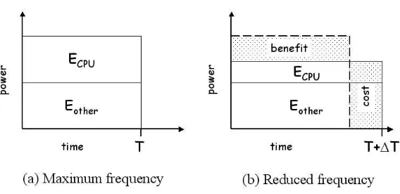
Figure 3.1: Cost Benefit Analysis of frequency reduction

the critical path due to bottlenecks at other components, and execute these sections of code at lower performance settings. The system power is seen as a function of frequency and is modeled asP(f) = PCP U(f) + Pother. However, energy is the product of (average) power

and time, so we consider the effect of frequency reduction has on elapsed time. Figure 3.1 shows the situation pictorially. When the program is run at the fastest gear, it takes time

T. On the right is a situation where the program is run in reduced gear taking time T

+ ∆T. The power savings is primarily a function of the frequency. Whether the lower frequency saves significant energy depends on whether the benefit due to power reduction is significantly greater than than the cost due to additional time. Essentially, this depends on ∆T/T: when it is small, there will be energy savings. Broadly speaking, ∆T/T is small when whole programs or enough phases of programs are memory, I/O, or communication bound. On the other hand, when most of the program is CPU bound, ∆T/T is large and little energy can be saved. In a parallel or distributed program, each node performs some work and usually contains one or more instances where two or more nodes synchronize with each other to exchange data or status information. Such instances are called synchronization points. If the node finishes its work by time T, and the synchronization happens at time

(21)

Intra-Node Bottleneck

Even though a superscalar processor can issue many instructions per cycle, peak utilization is hard to sustain for even short durations. A major source of this inefficiency is memory stalls: the microprocessor is underutilized because the memory system cannot immediately provide the data. In this case, the microprocessor is executing at a faster speed than necessary because of amemory bottleneck. The memory bottleneck exists largely because of the great improvement in microprocessors. Furthermore, attempts to eliminate this bottleneck, such as instruction scheduling, memory access reordering, and prefetching, have been met with limited success. This is also an issue with HPC, as memory can throttle the performance of an individual node. Therefore, reducing the performance of sections of the application which suffer from the memory bottlenecks can result in a significant energy savings with a small decrease in performance.

Another intra-node bottleneck is the I/O bottleneck. The I/O bottleneck occurs when computation is stalled waiting for I/O. This bottleneck provides two opportunities for saving energy. The first occurs because programs that are I/O bound have relatively low computation workloads. In this case, similar to the memory bottleneck, significant energy savings are possible by executing at reduced performance with potentially only a small performance decrease. However, there is an additional opportunity different from that provided by the memory bottleneck. Specifically, during blocked periods, it may be possible to achieve energy savings by switching to the lowest operating point—or even sleep mode—with no performance loss, because the node can make no progress anyway and the computational demand is low. Both these are considered intra-node bottlenecks since they exist independent of other nodes.

Inter-Node Bottleneck

(22)

F requency V oltage P ower(W)

(MHz) (V) idle active

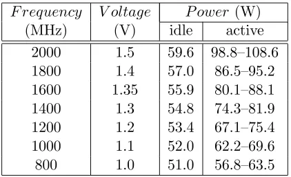
2000 1.5 59.6 98.8–108.6 1800 1.4 57.0 86.5–95.2 1600 1.35 55.9 80.1–88.1 1400 1.3 54.8 74.3–81.9 1200 1.2 53.4 67.1–75.4 1000 1.1 52.0 62.2–69.6

800 1.0 51.0 56.8–63.5

Table 3.1: Idle and active power for Athlon-64.

large body of work in parallelizing compilers as well as adaptation by parallel systems. Rather than eliminate these bottlenecks or increase parallel efficiency, our goal is to utilize the inevitable idle time to reduce energy consumed and heat generated. While it is difficult to so while incurring no increase in execution time, a significant reduction is possible with only a small performance degradation.

3.2 Methodology

Our experimental platform is a cluster of 10 nodes each with a frequency- and voltage-scalable AMD Athlon-64. Its available operating points are in the range of 800– 2000MHz and 0.9–1.5V, see Table 3.1. Each node has 1GB main memory, a 128KB L1 cache (split), and a 512KB L2 cache, and the nodes are connected by 100Mb/s network. In this paper, we vary the CPU power and measure overall system energy. Although there are other components, throttling the CPU is effective in saving energy because the CPU is a major power consumer. In particular, the Athlon-64 CPU used in this study consumes approximately 45–55% of overall system energy.1

The programs we studied included two of the ASCI Purple benchmarks [4] as well as all of the NAS suite [5]. Presumably, such mature benchmarks have been thoroughly analyzed and are well-written (e.g., see [54])—so some work has been done to balance the computational load. Therefore, well-tuned programs like those in ASCI and NAS should result in an approximate lower bound in terms of saving energy due to load imbalance. We

1_{CPU power is not measured directly. However, the system power at the fastest energy gear is 90–}

(23)

used as many nodes as possible on each test; this number is typically 8, though BT and SP run on 9 nodes.

For each program we measure execution time and energy consumed. Execution time is elapsed wall clock time. Total system power consumed by each node is measured by Watts-Up power meters at the wall outlet, which are connected to the serial ports of each node. These meters report average power consumption (in Watts) since last queried. Each node reads its associated meter every second and integrates power over time to determine the energy it consumes.

3.3 Results on the AMD cluster

In the results shown below, we used a cluster of ten nodes each with a frequency-scalable AMD Athlon-64. Table 3.1 shows the per-node system power consumption of different gears. We control the CPU power (by shifting gears) and measure overall system energy. This is effective in saving energy because the CPU—a major power consumer—uses less power. In particular, the Athlon CPU used in this study consumes approximately 55% of overall system power at 2000MHz and about 23% at 800MHz.

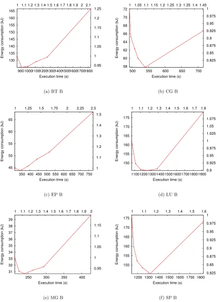
Single Processor Results

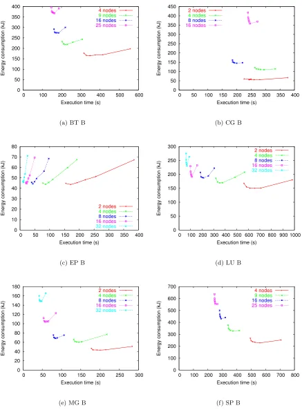
Figure 3.2 shows the results of NAS programs on a single Athlon-64 processor. For each graph, thetotal system energy consumed at each gear is plotted on the y-axis and the total execution time is plotted on the x-axis. The higher of two points uses more energy, and the further right of two points takes more time. Therefore, a near-vertical slope indicates an energy savings with little time delay between adjacent gears, whereas a horizontal slope indicates a time penalty and no energy savings. For readability, the origin of the graphs is not (0,0). Therefore, the alternate axes show the time and energy relative to the top gear (leftmost point). Because we tested the in-core version of NAS (i.e., class B), these programs do not have significant I/O.

(24)

130 135 140 145 150 155 160 165

900 1000 1100 1200 1300 1400 1500 1600 1700 1800 0.95 1 1.05 1.1 1.15 1.2 1.25 1 1.1 1.2 1.3 1.4 1.5 1.6 1.7 1.8 1.9 2 2.1

Energy consumption (kJ)

Execution time (s)

(a) BT B

58 60 62 64 66 68 70 72

500 550 600 650 700

0.825 0.85 0.875 0.9 0.925 0.95 0.975 1 1 1.05 1.1 1.15 1.2 1.25 1.3 1.35 1.4 1.45

Execution time (s)

(b) CG B

45 50 55 60 65

350 400 450 500 550 600 650 700 750 1 1.1 1.2 1.3 1.4 1.5 1 1.25 1.5 1.75 2 2.25 2.5

Execution time (s)

(c) EP B

150 155 160 165 170 175

1100 1200 1300 1400 1500 1600 1700 1800 1900 0.9 0.925 0.95 0.975 1 1.025 1.05 1.075 1 1.1 1.2 1.3 1.4 1.5 1.6 1.7 1.8

Execution time (s)

(d) LU B

31 32 33 34 35 36 37 38 39

250 300 350 400

0.95 1 1.05 1.1 1.15 1 1.1 1.2 1.3 1.4 1.5 1.6 1.7 1.8 1.9 2

Execution time (s)

(e) MG B

150 155 160 165 170 175

1200 1300 1400 1500 1600 1700 1800 0.825 0.85 0.875 0.9 0.925 0.95 0.975 1 1 1.1 1.2 1.3 1.4 1.5 1.6

Execution time (s)

(f) SP B

(25)

0 0.2 0.4 0.6 0.8 1 1.2

1 10 100 1000 10000

Beta

OPM

NAS

FP INT

Regression

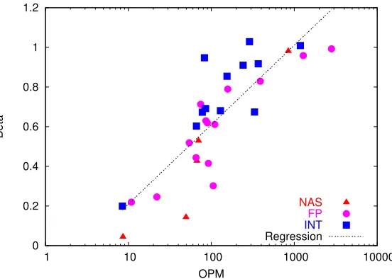
Figure 3.3: OPM v/s Beta for all benchmarks

other hand, EP at 1800MHz saves 2% energy with an 11% delay. This delay is the same as the increase in CPU clock cycle. EP is almost entirely CPU bound. Hence, inspection of CG and EP indicates that the challenge for system software is determining when to reduce the gear.

To quantify the degree of CPU (or memory) boundness, we use a metric calledβ, introduced in [26]. β is defined as a ratio between 0 and 1:

β = (T /Tmax−1) (fmax/f−1)

where T and Tmax are execution times at a lower frequency and maximum frequency

(2000MHz in this case), respectively, and f and fmax are the corresponding frequencies.

(26)

Phases(MHz) Time(s) Energy (KJ)

2000 2000 481 64.1

1800 1800 500 (+4%) 60.1 (-6.2%) 1600 1600 563 (+17%) 58.8 (-8.2%) 2000 1800 482 (+0%) 62.5 (-2.5%) 2000 1600 486 (+1%) 61.6 (-4.0%) 2000 1400 492 (+2%) 60.6 (-5.4%) 1800 1600 505 (+5%) 57.9 (-9.6%)

Table 3.2: Time and energy for different gears in different phases.

Multiple Processor Results

This section studies the effect of different gears on distributed programs. Figure 3.3 shows results for the NAS benchmarks. Each graph has the same general layout as in Figure 3.2, except that it shows the results from different node configurations. The energy plotted is the (measured) cumulative energy of all nodes used. These graphs show results using the samesingle gear on all nodes at all times. This shows that there are two tradeoffs to consider. One, which is similar to that on a single node, is the energy-time tradeoffwithin

a curve (different gears, same number of nodes). The second consideration, which is unique to multi-node configurations, is the energy-time tradeoff between curves (different number of nodes). Thus, there are now two dimensions to consider when trading performance for energy savings.

Figure 3.4 offers several examples where speedup is poor. In particular, this case is illustrated in SP from 2 to 4 nodes. When speedup is poor, cumulative energy increases because the number of nodes increases, so the main consideration is within a curve. The figure also shows an example where speedup is good (but not perfect or superlinear). Con-sider LU at 4 and 8 nodes. Gear 4 on 8 nodes uses approximately the same energy gear 1 on 4 nodes, but executes 50% faster. This is an important result, as it shows that there exist cases in which using more nodes with each node at a reduced gear can execute faster

and use less energy.

(27)

0 50 100 150 200 250

0 100 200 300 400 500 600

Energy Consumption (KJ)

Execution time (s)

1 node

4 nodes 9 nodes

(a) BT B

0 20 40 60 80 100 120 140 160 180

0 50 100 150 200 250 300 350 400

Execution time (s)

1 node

2 nodes 4 nodes 8 nodes

(b) CG B

0 10 20 30 40 50 60 70

0 50 100 150 200 250 300 350 400

Execution time (s)

1 node

(c) EP B

0 50 100 150 200 250

0 200 400 600 800 1000

Execution time (s)

1 node

(d) LU B

0 10 20 30 40 50 60 70 80

0 50 100 150 200 250 300

Execution time (s)

1 node

(e) MG B

0 50 100 150 200 250 300 350 400

0 100 200 300 400 500 600 700 800

Execution time (s)

1 node

4 nodes 9 nodes

(f) SP B

(28)

per phase we used a profile-directed technique described in detail in our prior work [19]. The table shows, for example, that we can save 5.4% energy with only a 2% increase in time with the two phases run at 2000MHz and 1400MHz, respectively. This is better in time than any fixed-gear solution (with the exception, of course, of running solely at 2000MHz) and saves nearly as much energy as any of the other fixed gear solutions.

(29)

Chapter 4

Simulation Model for Large

Clusters

The previous chapter presented results on our small power-scalable cluster. While the results are encouraging, it is left unclear what performance (in time and energy) can be expected for larger power-scalable clusters. Most likely, before building or buying a large power-scalable cluster, one would like to determine the performance potential. As we do not have access to more than ten nodes, this section seeks to address this issue by developing a simulation model.

4.1 Model

Understanding scalability of parallel programs is of course a difficult problem; indeed, it is one of the fundamental problems in parallel computing [48, 49]. Researchers try to predict scalability using a range of techniques, from analytical to execution-based. We will use a combination of both.

(30)

slower gears, we measure power consumption on a cluster node and use a straightforward algebraic formula. Below we describe our five-step methodology in full detail.

Step 1: Gather time traces. The first step is to gather active and idle times onnnodes

(TA₍_n_{) and}_TI₍_n_{), respectively, where}_TI₍_n_{) includes the actual communication time) on}

each of our clusters.

Step 2: Model computation and communication. The second step is to develop a

model of computation and communication that is based onTA₍_n_{) and}_TI₍_n_{). This will help}

us predict (in step 3)TA₍_m_{) and}_TI₍_m_{) where}_{m >}_10,_i.e_{, for power-scalable configurations}

with more than ten nodes. Our approach here is distinct for each quantity, out of necessity: no matter what the gear, the power consumed is different when computing than when blocking awaiting data.

DeterminingFp andFs. Here, we use Amdahl’s law to estimateFpandFs, which

denote the parallelizable and inherently sequential fractions of an application, respectively. For a test withinodes, we estimate Fp andFs as follows:

TA(i) = TA(1)(Fp/i+Fs)

Fp = 1−Fs

We obtain a family ofFp and Fs values. We will use these to determineFp and Fs on large

power-scalable clusters. Also, TA₍_n_{) represents the} _maximum _{computation time over all}

nodes.

Classifying communication. Here, we recall that TI _{includes idle time and}

communication time. While idle time (due to load imbalance) can be directly derived from

TA_{, the communication cost cannot. Hence, our approach is to categorize communication}

of each NAS program into one of three groups: logarithmic, linear, or quadratic. These are three common scaling behaviors for communication. To do this, we rely on three com-plementary methods: (1) inspection of the behavior of our measured TI _{on up to nine}

(31)

Step 3: Extrapolation of TA(m) and TI(m) at fastest gear. Third, we extrapolate to 16, 25, and 32 power-scalable nodes,i.e., m >10. For a given number of nodes, m, the sum ofTA₍_m_{) and} _TI₍_m_{) yields the execution time.}

Predicting active time: Predicting TA₍_m_{), requires an appropriate} _F

p and Fs

for 16 and 32 nodes on the power-scalable cluster. Using our measured values on up to 32 nodes on the Sun cluster and up to 9 nodes on our power-scalable cluster, we fitFp and Fs

for 16, 25, and 32 nodes on the power-scalable cluster using a linear regression.

Predicting idle time: Given the classification of communication behavior

(log-arithmic, linear, or quadratic) for each application, we use regression to fit a curve to the communication using measured data on power-scalable nodes. This gives us communication time on 16, 25, and 32 nodes.

Validation. Our technique is validated in the following way. For TA₍_m_{), we}

comparedFp and Fs on up to 9 nodes on both clusters. With only 1 exception, it was

iden-tical; the outlier was CG, where the parallelism actually increases from 4 to 8 nodes on our power-scalable cluster, but is constant on the Sun cluster. ForTI₍_m_{), each communication}

shape that we chose for our power-scalable cluster is identical on the Sun cluster up to 32 nodes. We also note that [54] supports our conclusion on five of the six programs. The exception is LU; for this program, we found that communication was best modeled as a constant; our traces showed that when nodes are added, each node sends more messages, but the average message size decreases.

Armed with estimates ofTA₍_m_{) and}_TI₍_m_{) on larger configurations (at the fastest}

gear), we now turn our attention to determining the effect of different energy gears on exe-cution time and energy consumption. The last two steps in this methodology are concerned with this issue.

Step 4: Determine Sg, Pg, andIg. The next step is to gather power data from a single

power-scalable node. Two values will be needed on a per-application and per-gear basis: application slowdown (Sg) and average power consumption (Pg). Separately, the power

consumption for an idle (i.e., inactive) system is determined for each gear (Ig).

This data determines the increase in time and the decrease in power. The execution time for a sequential program is wall clock time. This is done foreach (sequential) program at each energy gear. The ratio Sg is determined as follows: Sg = Tg(1)_T₁−₍₁₎T1(1). Now that we

(32)

The valuesPgandIgare obtained by measuring overall system power. The voltage

and current consumed by the entire system is measured at the wall outlet to determine the instantaneous power (in Watts). This experimental setup determines the values, Pg, for

each application and for each gear. The same setup, except this time with no application running, was used to determine the power usage of an idle system (Ig) at each gear.

Step 5: DetermineTg(m) andEg(m). The final step is to estimate the time and energy

consumption of a power-scalable cluster using the information developed so far. The time for a lower gear is computed by increasing the active time by the appropriate ratio, Sg.

We assume that executing in a reduced gear does not itself increase the idle time, as our experimentation has shown that the time for communication is independent of the energy gear—the computational load during MPI communication is quite low. Using the values of

Pg and Ig, we can estimate energy consumption at each lower gear for the MPI program.

In this straightforward case, the time and energy estimates, on mnodes, for each gear are:

Tg(m) = SgTA(m) +TI(m) (4.1)

Eg(m) = PgSgTA(m) +IgTI(m). (4.2)

At slower gears the compute time is greater than that of the fastest gear, whereas the idle time is independent of the gear. Thus the time executing in gear g increases to SgTA.

Communication latency is independent of gear, so this is assumed to remain the same. However, this naive case above is too simple because it assumes all computation is on the critical path. In many programs, not all computation is on the critical path. Of course, reducing the energy gear of any computation on the critical path will delay other nodes, who must wait for data sent from the (now slower) node. In the refined model,TA_is

classified intocritical andreducible work (TC _and_TR_{), and in our estimates of computation}

we separate these and estimate each. In short, executing reducible work in a slower gear mightnot increase overall execution time, because an increase in the time of reducible work will decrease the idle time. On the other hand, executing critical work in a slower gear always increases execution time. The communication latency, which is unaffected by CPU frequency, is delayed only by the slowdown applied to the critical work. The idle time is slack for the reducible work. However, if reducible work is slowed such that all slack is consumed, then the time will be extended. This point of inflection is whenTR+TI =SgTR.

(33)

computation between thelast send1 and a blocking point. In between those two points there is no interaction between nodes, so the work is not on the critical communication path. With this refinement, Equation (4.1) changes as shown below. Note that for notational simplicity, we omit number of nodes (m).

Tg =







Sg(TC+TR), ifTI+TR≤SgTR

Sg(TC+TR) +TI+TR−SgTR, otherwise

Then, Equation (4.2) becomes

Eg =







PgSg(TC +TR), ifTI+TR≤SgTR

PgSg(TC +TR) +Ig(TI+TR−SgTR), otherwise

4.2 Evaluation

Figure 4.1 shows the results of our simulation on each application ranging from 2–32 nodes. All node configurations up to and including 9 nodes are actual runs on the cluster, and configurations of 16, 25, and 32 nodes are simulated using the model discussed previously. (CG has a speedup of less than one on 32 nodes, so that curve is not plotted.)

In the same way that the eight- and nine-node tests tend to be more “vertical” than the two- and four-node tests, as with the runs up to nine nodes, the shapes of the graphs tend to become more “vertical” when using 16, 25, or 32 nodes;i.e., using lower gears becomes a better idea. As an example, consider SP. On four nodes, second gear consumes the least energy. On the other hand, on 16 nodes, fourth gear consumes the least energy.

One possible implication of this is that for massively parallel power-scalable clus-ters, the individual nodes can be placed in a relatively low energy gear with only a modest time penalty. As discussed in the previous section, this may potentially allow for supercom-puting centers to fit more nodes in a rack while staying within a given power budget. On the other hand, this could degrade performance significantly if many applications for such machines are embarrassingly parallel.

Second, speedup on the NAS suite generally starts to tail off around 25 or 32 nodes. Again, this is because this benchmark suite uses non-scaled speedup. The result of this is that the total cluster energy consumed starts to increase dramatically. Essentially, continuously increasing the number of nodes causes an application to be placed in the poor

(34)

0 50 100 150 200 250 300 350 400

0 100 200 300 400 500 600

Execution time (s)

4 nodes

(a) BT B

0 50 100 150 200 250 300 350 400 450

0 50 100 150 200 250 300 350 400

Execution time (s)

2 nodes

(b) CG B

0 10 20 30 40 50 60 70 80

0 50 100 150 200 250 300 350 400

Execution time (s)

2 nodes

32 nodes

(c) EP B

0 50 100 150 200 250 300

0 100 200 300 400 500 600 700 800 900 1000

Execution time (s)

2 nodes

32 nodes

(d) LU B

0 20 40 60 80 100 120 140 160 180

0 50 100 150 200 250 300

Execution time (s)

2 nodes

32 nodes

(e) MG B

0 100 200 300 400 500 600 700

0 100 200 300 400 500 600 700 800

Execution time (s)

4 nodes

(f) SP B

(35)

speedup classification (see previous section), which we know is energy inefficient. Also, for each application, there exists a certain number of nodes that, if exceeded, will cause program slowdown. It appears that that point is around 32 nodes for the NAS suite on our power-scalable Athlon-64 cluster.

This problem is not unique to power-aware computing; indeed, it is a problem with roots in the scalability field. However, it is clear that when this phenomenon occurs, it is necessarily the case that communication dominates computation. This means that in fact a lower gear is almost certain to be better. Hence, if one does not know what the parallel efficiency for a given application is, using a lower energy gear is a safeguard against excessive energy consumption.

(36)

Chapter 5

Just-in-Time Scaling

A parallel or distributed program usually contains one or more instances where two or more nodes synchronize with each other to exchange data or status information. We call these instances synchronization points. The node that is slowest to reach a synchronization point is considered the bottleneck node and is said to be on the critical path since it forces the remaining nodes involved in the synchronization to wait and is largely responsible for the duration of the synchronization. All other nodes are said to be non-critical, i.e. they have less or no influence on the duration of the synchronization. Typically, these non-critical nodes complete their work and wait for an event (e.g., a message) from another node. During this wait period the node is idle. Withjust-in-time (JIT) scaling, such a node executes at reduced performance and completes its work just before the message arrives from the remote node. Typically, a load imbalanced parallel program is one in which the workload of the program is not equally distributed among all the nodes or parallel processes. Since the workload is not equitably distributed, some nodes finish their allocated work earlier and wait at the above mentioned synchronization points for the slower nodes to catch up. This provides an opportunity to reduce performance on the non-critical nodes and save energy without a significant time-penalty to the entire application.

(37)

determine the optimal CPU speed for the latter such that their completion time is still less than that of the bottleneck node.

It is important to note that there is a trivial way to address this problem: for any early-arriving node, once it blocks at a synchronization operation, reduce its gear until the end of the synchronization operation. This is a simple scheme, yet it does not nearly produce optimal results in terms of energy savings. The reason is that the difference between consumed energy at different gears when a node is idle is much less than that difference when the node is active. For example, on our Athlon-64 nodes, the difference in power between the fastest and slowest gears is less than 10W when a node is idle and more than 30W when the node is active.

From the previous chapter we know that each communication and computation burst isTA₊_TI_{, where}_TA_{is the active time spent in computation and}_TI _{is the idle time}

spent in waiting for a remote node to respond. The active computation time consists of computation time that is critical and reducible,TA₌_TC ₊_TR_{. The reducible work can be}

slowed down as it does not significantly affect the overall time taken by the computation-communication burst. We can slow down the processor such that TA _{increases, reducing}

TI_{, keeping in mind not to increase the overall time of the burst. However, reducing}

the performance of the processor for every burst is infeasible since they are very small in duration and the overhead of determining if a gear shift should be made and the cost of shifting is significant compared to the duration of the burst. Therefore, we aggregate these computation-communication bursts for a significant time period and then decide if it allows for any reducible work.

Our programming model is as follows. We assume iterative programs, which com-prise the vast majority of scientific programs; furthermore, we assume that the iterations are relatively stable. This allows us to use past behavior to predict future behavior. For each nodei, each iteration takes timeTi, and consists of one or more compute-communicate

bursts. We denote the total compute time within one iteration asCi and the wait time or

slack time asWi, wherei is the node number (soTi =Ci +Wi). We monitor the wait time

(38)

communication operations. Consequently, reacting on a per-burst basis is too fine-grain. Therefore, Jitter considers all bursts in an entire iteration. By aggregating the the individ-ual wait times or each burst over the entire interval, Jitter determines the slack for each node over the entire interval, Si=Wi/Ti. The slack metric solves both issues.

We then calculate minimum slack of all the nodes —M inimumSlack=minimum(Si).

Net Slack is calculated as N etSlack = Si - M inimumSlack. If N etSlack = 0, then the

node is the bottleneck node and is on the critical path. As discussed above, the remaining nodes, which are not on the critical path, provide an opportunity to reduce gears if the resulting increase in compute time is less than the wait time,i.e., ∆C < S. A large amount of Net Slack indicates clearly that a node is not on the critical path and is a candidate for reduced performance. No or very little Net Slack indicates that the corresponding node provides no opportunity for frequency or voltage scaling.

Net slack is more useful than gross slack because a node with a net slack of 20% is clearly not a bottleneck whereas a node with 20% gross slack may actually be a bottleneck node. Also, the amount of slack per node can vary widely between different applications. For example, in the NAS suite average slack varies from less than 10% to over 90%. Second, the amount of slack per node can vary widely within an application and in practice is never zero on any node (because it is highly unlikely that any single node is always last to arrive at a large number of communication calls within an iteration).

The jitter algorithm only works for programs which are iterative and the behavior of the past iteration is a predictor for the next iteration. The jitter algorithm gathers information such as slack and iteration length over an iteration and uses this information to choose which gear the node should execute in for the next iteration. The decision it makes will be correct only if the next iteration has the behavior of the next iteration. Therefore, this discussion is limited to iterative programs (which is the vast majority of programs) where the past (usually) predicts the future.

Unfortunately, the existence of slack is not a sufficient condition to reduce the gear. There must be enough slack that reducing the performance will not increase the execution time too much. Armed with the normalized slack per node, our system reduces the performance of each node that has enough slack such that reducing the gear is unlikely to increase the execution time. Our algorithm is then adaptive in that if the gear reduction was too much, we increase the gear; if it was too little, we further reduce the gear.

(39)

appli-cation and the MPI Library. It is an interface that exploits PMPI [44] the profiling layer of MPI. MPI-Jack enables a user transparently to intercept (hijack) any MPI call. A user can execute arbitrary code before and/or after an intercepted call usingpreandpost hooks. In this work, we use MPI-Jack to determine the time spent in blocking MPI calls, such as

MPI Recv,MPI Wait, andMPI Barrier. The pre hook records the time the routine began. The post hook records when it ends, computes the wait time, and updates the node’s overall wait time. Our MPI-Jack library is dynamically linked to the application during the process of compilation. When the application executes, all MPI calls made by the application are trapped by the MPI-Jack library.

To make an effective decision for reducing performance of non-critical nodes, there are several items that Jitter must determine:

• the iteration boundaries,

• the net slack of each node,

• when to reduce the performance,

• when to increase the performance,

• when to remain in the same gear,

• when to reset algorithm parameters, and

• how to determine the threshold slack

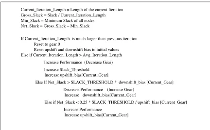
We describe each of these in turn. The Jitter Algorithm is given in pseudocode in Figure 5.1.

Determining the iteration boundaries Currently, we manually insert a special Jitter

MPI call, MPI Jitter, at the top of the main loop in the program; however, this is easily automated [28]. Such a loop must exist, as we are assuming iterative programs. When itera-tions are too short, Jitter limits the overhead by waiting several iteraitera-tions beforeMPI Jitter

takes action. Thus is also done in order to amortize the overhead of Jitter and because there is little benefit to reducing performance for only a short period. The current implementation combines iterations until the time exceeds half a second. Jitter performs several actions in

MPI Jitter, which are described next.

Determining the net slack of each node Slack in Jitter is determined as follows.

(40)

Gross_Slack = Slack / Current_Iteration_Length

Net_Slack = Gross_Slack − Min_Slack

Current_Iteration_Length = Length of the current Iteration

Min_Slack = Minimum Slack of all nodes

Reset to gear 0

Reset upshift and downshift bias to initial values

If Current_Iteration_Length is much larger than previous iteration

Else if Current_Iteration_Length > Avg_Iteration_Length

Else If Net_Slack > SLACK_THRESHOLD * downshift_bias [Current_Gear] Decrease Performance (Increase Gear)

downshift_bias[Current_Gear] Increase

Increase Performance (Decrease Gear) Increase Slack_Threshold

Increase upshift_bias[Current_Gear]

Else if Net_Slack < 0.25 * SLACK_THRESHOLD / upshift_bias [Current_Gear] Increase Performance

Increase upshift_bias[Current_Gear]

Figure 5.1: The Jitter algorithm

then compute the absolute or gross slack as the ratio of the wait time divided by the

iteration time. The global minimum slack among all nodes is determined using a reduction (MPI Allreduce). Then the node’s net slack is computed as the difference between itswait time and the global minimum. The need to usenet slack has been explained in Chapter 5.

Determining when to reduce performance Jitter reduces a node’s performance if

there is enough net slack. The Jitter prototype uses the following relationship to determine whether there is enough slack to reduce the gear:

net slack> S·dg →enough slack.

(41)

While net slack is better than gross slack at identifying a bottleneck node, it is not enough. If Jitter chooses to reduce and it turns out to be a bad choice (which is learned when the node later observes a large increase in execution time and so increases performance) the threshold to reduce again is raised. This threshold increase is captured in the term dg, which we call the downshift factor. Each time a node reduces from gear g

it increasesdg using the formula dg =dg∗bias. Through experimentation, we found that

a bias = 1.5 worked well for all applications. We have not found that the benchmarks are very sensitive to the bias value; however, further experiments are ongoing.

Determining when to increase performance Each node determines if it is a

bottle-neck node according to the following relationship.

net slack< α·S/ug →bottleneck node.

The termαis used to ensure the possibility that Jitter can inform a node to remain in the same gear. Although it could be a user-provided parameter, we use α= 0.25 in our tests. This simplifies use and has little adverse effect on Jitter’s performance. We use an

upshift factor, ug, that is similar in spirit to the downshift factor above. It is adjusted each

time there is an increase in performance using bias in the same way asdg. This lowers the

threshold slack required to shift up.

Because there is always at least one bottleneck node every iteration, being a bot-tleneck node is not a sufficient condition for increasing performance, for two reasons. First, a node can be a bottleneck in a lower gear without slowing down the computation. This happens when there is another node that is as slow or slower but is in the top gear. Second, there is variance in the times between iterations even in the best situation. Therefore, some conditions are transient and we do not want Jitter to react to them.

Consequently, a bottleneck node will increase its performance if either of the fol-lowing conditions hold: (1) the iteration time has increased, and the node reduced its gear on the previous iteration, or (2) the node has been a bottleneck for three consecutive iterations.

Determining when to remain in the same gear Jitter remains in the same gear

(42)

net slack < S. The more the algorithm shifts gears, the larger this range is, due to the biasing of the upshift and downshift factors. Thus the algorithm tends to stabilize.

To prevent a form of “thrashing”, where the gear constantly changes, we use thresholds in the following way. If a node reduces the gear too far, we increase the threshold value for reducing the gear. That threshold is decreased if there is extra slack time still remaining after a gear reduction. However, we increase the threshold by more when the gear is reduced too far than we decrease it when the gear is not reduced too much—this is because we bias towards high performance for HPC applications. Our system learns the proper thresholds for each application at runtime.

Determining when to reset algorithm parameters In addition to the above three

standard actions (reduce, increase, remain), there is a fourth, extraordinary action, which is to reset the algorithm parameters. This action is triggered by a dramatic change in the iteration time. Currently, a reset occurs if the time between adjacent iterations changes by 50% or more. The reset is not because of a problem within Jitter, but rather because because the application has changed in a significant way. (Jitter only otherwise changes by a single gear per iteration, which is not likely to cause a large change because frequencies change by 20% or less between adjacent gears.) None of the tested NAS or ASCI benchmarks algorithms causes a reset; however, we force a reset with our synthetic benchmark (see the next section).

How to determine the threshold slack Our Jitter algorithm chooses to reduce

(43)

would be fix at the rate of change of the frequency.

Hence, the slack threshold is difficult to determine without prior knowledge of the application. Therefore it was necessary to design Jitter such that is would dynamically determine the slack threshold for each of the applications. The algorithm begins with an initial slack threshold of 0.05, which signifies that if a node has 5% net slack, Jitter should consider it as a candidate to reduce performance. This slack threshold is only incremented when the algorithm decides to decrease performance for a particular node due to overall increase of the program time. When the threshold slack is incremented, e.g to 0.07, Jitter will only consider this node as a candidate to decrease performance only if its net slack is greater than 7%. Since the algorithm is designed in such a way that that it stabilizes after initial few iterations, the slack threshold also stabilizes to provide optimum energy-time trade-off. The slack threshold is further examined in the next chapter. .

(44)

Chapter 6

Jitter Results

In this section, we present the Jitter results. We show the benefits of Jitter on imbalanced applications. Then, using a synthetic benchmark, we show the full capabilities of Jitter. Last, we show that Jitter does not slow down a program unnecessarily when its load is balanced. We also evaluate the overhead and sensitivity of the Jitter implementation.

6.1 Non-Uniform Loads

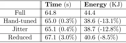
This section shows the results of two benchmark programs that have load imbal-ance. The first one, Aztec, is a parallel iterative solver for sparse linear systems from the Purple suite. Table 6.1 shows results for Aztec using four different methods. All results are the average of at least 3 runs, with little variance. The first method isFull power, where all nodes execute in top gear (2000MHz). It is used as the baseline. The next uses ahand-tuned

set of per-node gear settings. Using the slack on each node at Full as a guide, we tested many solutions to find the “best.” Because we are biasing towards performance, the goal was to save as much energy as possible while allowing only small performance impact, which

Time(s) Energy (KJ)

Full 64.8 44.4

Hand-tuned 65.0 (0.3%) 38.6 (-13.1%) Jitter 65.1 (0.4%) 38.7 (-12.8%) Reduced 67.1 (3.0%) 40.6 (-8.5%)

(45)

800 1000 1200 1400 1600 1800 2000

0 10 20 30 40 50 60 70

Frequency

Iteration

0

1 23 45 67

Figure 6.1: Gears for chosen by Jitter for Aztec.

we somewhat arbitrarily define as less than 2.5% increase in time. While our search was not exhaustive, it was extensive. The third method is Jitter, where all nodes begin in top gear and dynamically shift according to the algorithm described in the previous chapter. In the last method (Reduced), every node executes at 1800MHz—performance is reduced by one gear. This method serves as another baseline.

The hand-tuned run saves 13% energy with no time penalty. Each node executes in a single, but possibly different gear: one node runs in top gear (node 4), four in 1800MHz (nodes 1, 2, 3, and 5), and one each in the next three gears. (Frequency is used to name the gear, but both frequency and voltage are scaled.)

The Jitter run takes more time than Full, but saves nearly 8% energy. As expected, it does not save as much energy as the hand-tuned method. The primary reason for this is that the gears selected by the algorithm are higher than in hand-tuned. Five of the nodes execute more than half of the iterations in top gear. The secondary reason is the cost of constantly shifting gears, as it takes Jitter a handful of iterations to determine a solution. During this time it continually refines the gear settings. It should be noted that Aztec is the least stable of all benchmarks—e.g., it still shifts to some extent after 50 iterations—which we believe is likely typical of a production application than the other benchmarks.

(46)

800 1000 1200 1400 1600 1800 2000

0 50 100 150 200

Frequency

Iteration

0

1 23 45 67

Figure 6.2: Gears for each node for each iteration in Sweep3d.

cycle it becomes harder to reduce due to the increasing downshift factor dg. Our goal of

favoring performance over energy forces these nodes into the top gear. Nevertheless, Jitter performs well. It is possible to extract better numbers from Jitter by tuning the parameters to optimize it for Aztec; however, this paper presents a more general usage of Jitter.

Figure 6.1 shows the gears per node per iteration for Aztec. It shows a single, representative run. Because there are more nodes than gears, the lines overlap significantly. At the end there are 5 nodes that execute at 2000MHz (nodes 1–5). Node 7 reduces one gear each iteration down to 1000MHz, where it remains for the duration of the program’s execution. Node 0 predominantly executes at 1200MHz and node 6 at 1400MHz.

The second program that shows load imbalance isSweep3d, which is also a Purple benchmark. Sweep3d solves a time-independent discrete geometry neutron transport prob-lem in 3-dimensions. Table 6.2 shows the results. In the hand-tuned method two nodes, 6 and 7, are in 1800MHz, while the rest are in top gear. There is essentially no time penalty for hand-tuned. Even with this little difference from full performance, there is a noticeable energy savings.

Time(s) Energy (KJ)

Full 26.2 19.1

(47)

600 800 1000 1200 1400 1600 1800 2000

0 5 10 15 20 25 30 35 40

Frequency

Iteration

0

1 23 45 67

Figure 6.3: Gears for each node for each iteration in synthetic benchmark with stable, non-uniform load.

Time(s) Energy (KJ)

Full 80.0 55.1

Table 6.3: Synthetic benchmark results

Figure 6.2 shows the gears used by Jitter in Sweep3d. Because the application iteration length is about 0.1 seconds, Jitter takes action only every 5 iterations; therefore, the figure plots every 5 iterations. It stabilizes much more quickly than Aztec, reaching stability within 50 iterations (10 Jitter iterations). After iteration 50, the nodes are in the same gears as hand-tuned. Before that, 4 different nodes reduce to 1600MHz, two of which climb back to top gear. Overall, 89% of the time Jitter is in the same gear as hand-tuned, and only 2% of the time are any nodes more that one gear away from hand-tuned. Therefore, Jitter performs nearly the same as hand-tuned.

6.2 Synthetic Benchmark Results

(48)

0 0.1 0.2 0.3 0.4 0.5 0.6 0.7 0.8

0 5 10 15 20 25 30 35 40

Slack Iteration 0 1 2 3 4 5 6 7

Figure 6.4: Slack for each node and each iteration in synthetic benchmark with stable, non-uniform load. 0 1000 2000 3000 4000 5000 6000 7000 8000 9000

0 1 2 3 4 5 6 7

Energy consumed (Joules)

Node

Full Hand-tuned Jitter

Figure 6.5: Energy consumed for each node in synthetic benchmark with stable, non-uniform load.

executes a barrier.

Figure 6.3 shows gears for each node. In this example, each node has an increasing amount of work, so node 0 has the least work and node 7 the most. Through separate experimentation, we determined these loads so that each node should select a different gear. (Because there are only 7 gears, 0 and 1 should select the same gear).

Table 6.3 shows the overall results. As expected, when using Jitter, there is sig-nificant energy savings and little time penalty. Jitter is nearly the same as the hand-tuned case because it stabilizes quickly to the same gear assignments as hand-tuned.

(49)

600 800 1000 1200 1400 1600 1800 2000

0 5 10 15 20 25 30 35 40

Frequency

Iteration

0

1 23 45 67

Figure 6.6: Gears for each node for each iteration in synthetic benchmark with unstable, non-uniform load.

much load as node 1, still has a significant amount of slack. However, five nodes have less than 10% slack. There is spike at iteration 12 that we cannot explain. Apparently, all communication takes longer in this iteration. Every node’s total wait time increases about the same amount (15ms). This spike is seen in every run (but different iterations) of the synthetic benchmark for all methods and every run of MG (from the NAS benchmark suite). These are the only programs that have several nodes with less than 10% slack. It is possible that there is a transient delay in the network that programs with more slack are able to absorb, which is why we do not see spikes in other programs.

Figure 6.5 shows the energy consumed by each node for the three methods. The less loaded nodes use significantly less energy when using Full because Linux issues aHALT

instruction during idle. The figure shows that the most energy is saved in these lower loaded nodes. Importantly, for this program, Jitter achieves nearly the same results as the hand-tuned method.