ESTIMATION OF MULTIPLE FREQUENCY & PHASE USING OBSERVER AND ESTIMATOR

(1)

A Monthly Double-Blind Peer Reviewed Refereed Open Access International e-Journal - Included in the International Serial Directories

International Journal in IT and Engineering

http://www.ijmr.net.in

email id- [email protected]

Page 196

ESTIMATION OF MULTIPLE FREQUENCY & PHASE USING OBSERVER AND ESTIMATOR

Deepali Verma*

Amit Goriyan**

Akhilesh Singh***

*M.Tech Student, Deptt. of EEE, GRDIMT, Dehradun. ([email protected])

** Assistant Professor, Deptt. of EEE, GRDIMT,Dehradun.

*** Assistant Professor, Department of EEE, Simant Engg. College,Pithoraghar.(Uttarakhand).

ABSTRACT

In signal & system, designing and development of off-line and on-line estimator is the basic problem.

The recent advancement in control system developed on-line frequency estimators in various

operations. The complication in estimating unknown frequencies of a complex sinusoidal signal

simultaneously is our basic research purpose. In our work, different estimators are analyzed on the basis

of on-line estimation. The presented estimators ensure a continuous time on-line simultaneous

frequency estimation, which guarantees global boundedness and convergence of the state and

frequencies estimation for all initial conditions and frequencies.

(2)

International Journal in IT and Engineering

I.INTRODUCTION

In this, we address the problem of simultaneous online estimation of the state and the frequency of a

measurable multiple sinusoidal signal composed of the sum of n sinusoidal terms given by

𝑦 𝑡 = 𝑛𝑖=1𝐴𝑖 𝑠𝑖𝑛(𝑎 𝑖𝑡 + ∅𝑖)

Here Y(t) is a signal, 𝐴0≠ 0,the frequency 𝜔𝑖 ≠ 0 𝑎𝑛𝑑 and the initial phases are unknown for i=1,2……,n.

The frequencies are different from each other. The frequency estimation is a most critical problem in

control theory, due to the number of practical applications in rotational mechanical processes like, disk

drivers, induction motors helicopters or controlling of vibration among others ([2], [4], [6], [7]).

The issue of estimation of the frequency of any signal has been studied extensively by means of different

techniques both in the offline case [11] and the online estimation [8], but just a while ago, a globally

convergent estimator was proposed in [1] on the basis of an adaptive notch (AN) filter first proposed in the

discrete-time version in [8] and adapted in for the continuous-time case [2]. A key feature of this Adaptive

Notch filter was the scaling of the forcing term to normalize the parameters, which does not affect stability

and ensures the positivity for all time of the estimate.

The problem of simultaneous online convergent estimation of the frequency and the state is a notable

problem in system & control theory. In our work, we propose a solution to this well known problem and

then extend the results naturally to the case of n unknown frequencies. More precisely, we present a new

estimator which ensures a continuous-time online simultaneous frequency and state estimation, securing

that all signals are globally bounded and the estimation of the frequencies and the states are

asymptotically correct for all initial conditions and frequency values. In short we discuss this results and

the difference with the approach presented in this paper .

II. ESTIMATION USING ADAPTIVE OBSERVER

Consider a sinusoidal signal

𝑦 𝑡 = 𝐴1 sin(𝑎1𝑡 + ∅1)

For this we can generate a state model

(3)

International Journal in IT and Engineering

email id- [email protected]

Page 198

𝑥2(t) = -a2 x1(t)

y t =𝑘1

𝜆 𝑥1 + 𝑘2

𝜆 𝑥2

in which the parameter 𝑎2_{is unknown, k1, k2,λ 0 and the initial conditions are also unknown. The}

parameter is introduced here to scale the magnitude of the signals.

We are interested in the estimation of the state(x1,x2) and the frequency 𝑎2.

Let state of the estimator is denoted by ( s1 , s2 ,s3)T.

Error e = (e1, e2, e3)T.

With e1= x1- s1

e2= x2 - λs₂

and e3= s3 – a2

Proposition 1: The estimator structure can be proposed as:-

𝑠′1 = 𝜆𝑠2+ 𝜆

𝑘2 (𝑦 − 𝑦 )

𝑠′2= − 𝑆1𝑆3

𝜆 + 𝜁 (𝑦 − 𝑦 )

_𝑠_′₃= −𝛾𝑠1(𝑦 − 𝑦 )

𝑦 = 𝑘1

𝜆 𝑠1 + 𝑘2𝑠2

Where

  

, ,



0and ,

k k

1 2



0

ensure that lim𝑡→∞𝑒 = 0.

Proof: The error dynamics takes the

𝑒′1 𝑡 = −𝑘1

𝑘2 𝑒1

𝑒′

2 𝑡 = −𝑒1 𝑎2+ 𝜁 𝑘1 − 𝜁𝑘2𝑒2+ 𝑒3𝑠1

𝑒′

3 𝑡 = − 𝛾

𝜆𝑠1(𝑘1𝑒1+ 𝑘2𝑒2)

Let us take Lyapunov candidate function

𝑉 𝑒 = 𝑒𝑇𝑀𝑒 = 𝑒𝑇 𝑐1

2 𝑘1

2 0

𝑘1

2 𝑘2

2 0

0 0 𝜆

2𝛾

(4)

International Journal in IT and Engineering

email id- [email protected]

Page 199

M is Hermitian matrix, we know that M is definite-positive if

c

1



0

and

2

1 2 1

c k k from which

k

₂ must be positive.

The derivative of V e

 

is now calculated as

𝑉 (e)= 𝑐₂1 𝑒 1 2+ 𝑘2

2 𝑒 2

2₊ 𝜆

2𝛾 𝑒 3

2_{+ 𝑘}

1 𝑒1 𝑒2

= 𝑐1

2 𝑒 1 𝑒1 + 𝑘2

2 𝑒 2 𝑒2 + 𝜆

2𝛾 𝑒 3 𝑒3 + 𝑘1 𝑒1 (𝑒2) + 𝑘1 𝑒2 (𝑒1)

Fig. 1: Signals S1 , S2 , S3 for a = 1

𝑉 (e)= 𝑐1 2 𝑒1

−𝑘1

𝑘2 𝑒1 +

𝑘2

2 −𝑒1 𝑎

2_{+ 𝜁 𝑘}

1 − 𝜁𝑘2𝑒2+ 𝑒3𝑠1 𝑒2 + 𝜆

2𝛾 −

𝛾

𝜆𝑠1 𝑘1𝑒1+

𝑘2𝑒2𝑒3+[𝑘1−𝑘1 𝑘2 𝑒1𝑒2]+[𝑘1{−𝑒1𝑎2+𝜁 𝑘1−𝜁𝑘2𝑒2+𝑒3𝑠1}(𝑒1)]

By solving this equation:-

𝑉 (e) = −𝑒12[ 𝑐1𝑘1

𝑘2 + 𝑎

2_𝑘

1+ ζ 𝑘12] − 𝜁𝑘22𝑒22− 𝑒1𝑒2[𝑘2𝑎2+ 𝑘12

𝑘2 + 2𝜁𝑘1𝑘2]

(5)

International Journal in IT and Engineering

email id- [email protected]

Page 200 𝑐₁𝑘₁

𝑘₂ + 𝑎

2_𝑘

1+ ζ 𝑘12 >

𝑘₂𝑎2₊𝑘12 𝑘2+2𝜁 𝑘1𝑘2

4𝜁 𝑘₂2

To satisfy both conditions 2

1 2 1

c k k and (3.16), following constraint is imposed:

𝑐1> 𝑚𝑎𝑥 𝑘12

𝑘2 , 𝑘2

𝑘1

𝑘2𝑎2+𝑘1 2

𝑘2 + 2𝜁𝑘1𝑘2 4𝜁𝑘22

2

− 𝑘1𝑎2− 𝜁𝑘12

Since 𝑉 𝑖𝑠 𝑛𝑜𝑡 𝑛𝑒𝑔𝑎𝑡𝑖𝑣𝑒 𝑑𝑒𝑓𝑖𝑛𝑖𝑡𝑒

Now, 𝑉 =0 is the set

Ω = ,(e,s) I 𝑒1= 𝑒2= 0}

To show the stability of error dynamics, the solution of the error dynamics and estimator in set is given by

𝑠1=λ 𝑠

𝑠2= -𝑠1 𝑠2

𝜆

𝑠3=0

𝑒2 = 0 = 𝑠1𝑒3

𝑒3= 0

From this, we can observe that,

e

₃ must be zero, since

e

1



0

so

e

3



0

and the error dynamics tends

asymptotically to zero. It leads to conclusion that s3 tends asymptotically to the value of 𝑎2_{. So, in the}

invariant set, the only solution for the error dynamics is the trivial solution and for the observer dynamics, the only solution is a limit cycle and the output is precisely the exact output of the original system. So, since V e

 

is radically unbounded for all the values ofe, by using the Lasalle-Krasovskii theorem [4], we

(6)

International Journal in IT and Engineering

email id- [email protected]

Page 201

III. For n-FREQUENCIES

In this, we depict the extension of the signal containing

n frequencies and given by

𝑦 𝑡 = 𝐴𝑖 𝑛

𝑖=1

sin 𝑖𝑡 + ∅𝑖

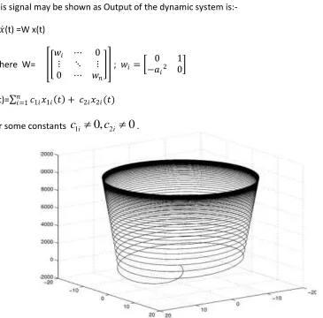
This signal may be shown as Output of the dynamic system is:-

𝑥 (t) =W x(t)

Where W=

𝑤𝑖 ⋯ 0

⋮ ⋱ ⋮

0 ⋯ 𝑤𝑛

; 𝑤𝑖 = _−𝑎0 1

𝑖2 0

Y(t)= 𝑛𝑖=1𝑐1𝑖𝑥1𝑖 𝑡 + 𝑐2𝑖𝑥2𝑖(𝑡)

for some constants

c

1i



0,

c

2i



0

.

Fig. 2: signals s1, s2, and s3 for a=100.

State model can be developed as:-

𝑥1 = 𝑥2

𝑥2 = 𝑥3

(7)

International Journal in IT and Engineering

email id- [email protected]

Page 202

𝑥 2n-1 = 𝑥2𝑛

𝑥2𝑛 = −𝑎0𝑥1− 𝑎2𝑥3− ⋯ − 𝑎2𝑛 −2𝑥2𝑛−1

Where 𝑎0= 𝑛𝑖=1𝑎𝑖2 and 𝑎2 = 𝑛𝑖=1𝑎𝑖2

Output 𝑦 𝑡 = 1 𝜆𝑗 2𝑛 −1

𝑗 =1 𝑘𝑖𝑥𝑖

2𝑛 𝑖=1

𝑎0 and 𝑎2are the coefficients of the characteristics polynomial

Theorem-3:- The estimator is shown as:-

0 𝜆1 0 ⋯ 0 0 0

𝑠 (t)= 0 0 𝜆2 0 0 s(t) + 0 (y-𝑦 )

⋮ ⋮ ⋮

0 0 0 0 𝜆2𝑛−1 𝑔1

−𝑆2𝑛 +1

𝜆𝑗 2𝑛 −1

𝑗 =1 0

−𝑆2𝑛 +2

𝜆𝑗 2𝑛 −1 𝑗 =3 ⋯

−𝑆2𝑛 +𝑛

𝜆2𝑛 −1 0 𝑔2

𝑆 2n+1= −𝑔3𝑠1(𝑦 − 𝑦 )

𝑆 2𝑛 +2 = −𝑔4𝑆3(𝑦 − 𝑦 )

⋮

𝑆 2𝑛 +𝑛=−𝑔𝑛 +2𝑆2𝑛 −1(𝑦 − 𝑦 )

With 𝑔𝑖 > 0 for i=2,3,4….n+2 , 𝑔1= 𝜆2𝑛 −1

𝑘2𝑛 𝑦 = 𝑘𝑖 𝜆𝑗 2𝑛 −1 𝑗 =𝑖 2𝑛−1

𝑖=1 + 𝑘2𝑛𝑆2𝑛

And 𝑘𝑖 chosen such that polynomial:-

P(w)=𝜔2𝑛 −1₊𝐾2𝑛 −1

𝑘2𝑛 𝜔

2𝑛 −2₊𝑘2𝑛 −2

𝑘2𝑛 𝜔

2𝑛 −3_{+ ⋯ +} 𝐾2

𝐾2𝑛𝜔 +

𝐾1

(8)

International Journal in IT and Engineering

email id- [email protected]

Page 203

Is stable with all its roots distinct is such that 𝑦 = 𝑦,

𝑠2𝑛 +𝑖 → 𝑎2𝑖−2 , For i=1,2 ….n when t→∞

Proof:- Consider the error system first:-

𝑒1= 𝑥1− 𝑠1

𝑒1 = 𝑒2= 𝑥2− 𝜆1𝑠2

𝑒2 = 𝑒3= 𝑥3− 𝜆1𝜆2𝑠3

⋮

𝑒 2𝑛−1= 𝑥2𝑛 − 𝜆1𝜆2… 𝜆2𝑛−1𝑠2𝑛 − 𝜆1𝜆2…𝜆2𝑛−2𝑔1(𝑦 − 𝑦 )

Fig.3: signals x5,x6,a0,a1

(9)

International Journal in IT and Engineering

email id- [email protected]

Page 204

Characteristics polynomial:-

P(w)= 𝑤2𝑛 −1+𝑘2𝑛 −1

𝑘2𝑛 𝑤

2𝑛 −2₊𝑘2𝑛 −2

𝑘2𝑛 𝑤

2𝑛 −3_{+ ⋯ +} 𝑘2

𝑘2𝑛𝑤 +

𝑘1

𝑘2𝑛 and is stable by hypothesis. Error dynamic

may be rewritten as:- 𝑒 1 = 𝐴𝑒1

𝑒4 = −𝛽1𝑇𝑒 1− 𝛽2𝑒2𝑛+ 𝑠 1𝑇𝑒 3

𝑒 3= −𝛤𝑠 1(𝑘 1 𝑇

𝑒 1+ 𝑘2𝑛𝑒2𝑛) Where A is a Hurwitz and given by

0 1 ⋯ 0

A= 0 0 ⋯ ⋮

0 0 1

−𝐾1

𝐾_2𝑛 −𝐾₂ 𝐾_2𝑛 ⋯

−𝐾_{2𝑛 −1} 𝐾_2𝑛

Matrix A has distint eigen values then there exist a matrix T such that:-

𝐴 = 𝑇−1_{𝐴𝑇 = 𝐷𝑖𝑎𝑔 (}_µ

1µ2…µ2𝑛−1)

𝑒 1= 𝑇𝑒1

And the error dynamics take the form:-

𝑒 1= 𝐴 𝑒 1

𝑒 2𝑛 = −𝛽 1 𝑇

𝑒 1− 𝛽2𝑒2𝑛+ 𝑠 1𝑇𝑒 3

𝑒 3= −𝛤 𝑠 1(𝑘 1 𝑇

𝑒 + 𝑘1 2𝑛𝑒2𝑛)

Where 𝛽 1 𝑇

= 𝛽𝑇₁𝑇 𝑎𝑛𝑑 𝑘 1 𝑇

= 𝑘 𝑇1𝑇

Since 𝐴 𝑖𝑠 𝑑𝑖𝑎𝑔𝑜𝑛𝑎𝑙 ,there exist a Lyapunov function 𝑣0 𝑒 1 satisfying :-

𝑣0 𝑒 1 = 𝑒 1𝑇𝑃𝑒 1

(10)

International Journal in IT and Engineering

email id- [email protected]

Page 205

For some P,Q diagonal and positive definite. Let us now consider the Lyapunov candidate function:-

V(𝑒 1, 𝑒2𝑛, 𝑒3)= 𝑣0 𝑒 1 + 𝐶12𝑇𝑒 1𝑒2𝑛+ 𝐶2𝑛 𝑒2𝑛2

2 +

1 2𝑒 3

𝑇_𝐶

3𝑒 3

With 𝐶12 = [𝐶1,2𝑛 𝐶2,2𝑛 𝐶2𝑛 −2,2𝑛]T

𝐶3= 𝐷𝑖𝑎𝑔 𝐶13 𝐶23… 𝐶𝑛3 Which is a positive definite for some P and 𝑒2𝑛 > 0.

Fig.4: Signal y,𝑦

From this, we have third equation:-

𝑉 𝑒 1, 𝑒4,𝑒 3 =

−𝑒 1𝑇(𝑄 + 𝐶12 𝛽 1 𝑇

) 𝑒 1− 𝐶2𝑛𝛽2𝑒2𝑛2− (𝐶12𝑇𝛽2− 𝐶12𝑇𝐴 + 𝛽 1 𝑇

𝐶2𝑛)𝑒 1𝑒2𝑛+ (𝑒 1𝑇𝐶12)(𝑆 1 𝑇

𝑒 3)𝑒2𝑛 -

(𝑒 1𝑇𝑘 1)(𝑠 1𝑇𝛤𝐶3𝑒 3)+ 𝐶2𝑛 𝑠 1𝑇𝑒 3 𝑒2𝑛− 𝑘2𝑛𝑠 1𝑇𝛤𝐶3𝑒 3𝑒2𝑛

Choosing C2n=k2n

C12=𝑘 1

(11)

International Journal in IT and Engineering

email id- [email protected]

Page 206

Finally, we get:-

𝑉 𝑒 1, 𝑒2𝑛,𝑒 3 = −𝑒1𝑇 𝑄 + 𝑘 1𝛽 1 𝑇

𝑒 1− 𝑘2𝑛𝛽2𝑒2𝑛2− (𝑘 1 𝑇

𝛽2− 𝑘 1 𝑇

𝐴 + 𝛽 1 𝑇

𝑘2𝑛) 𝑒 1𝑒2𝑛

This is negative semi definite for the any value of Q.Therefore we use the same analysis made in the single

frequency case. In this case the invariant set in gain by 𝑒 1= 0, e2n=0 and 𝑒 3must be zero b’coz the

assumption that frequencies are distint implies that the signals are linearly independent .

IV. SIMULATIONS RESULT

The performance of the estimator was tested by simulations, some of which are presented in the

following figures. Firstly, we can show in Fig. 1 the behavior of the estimator for a single frequency

λ= 1, = 10, = 1, k1 = 1, k2 = 1, = 1 and y(t) = sin(a t) we can see the fact that if the frequency is increased,

then the magnitude of x increased, therefore, we can increase to reduce the magnitude of s and reduce k2

and k1 for which the dynamics of s1 are faster. The response of the estimator for a= 100, where the

parameters are k1 = 0:5, k2 = :25, λ= 100, γ= 1000, ζ= 1000 and y(t) = 10 sin(100t) is shown in the Fig. 2.

We observe the good behavior of the estimator.

Taking now two frequencies, let us say a1 = 1,a2 = 2, we get a0 = 4 and a2 = 5 and the performance of the

filter with parameters k1 = 6, k2 = 11, k3 = 6, k4 = 1,λ = 1 and y(t) = 10(sin(t) + sin(2t)), are shown in Figs. 3

and 4.As it may be seen, the estimator exhibits a good convergence property, so these results suggest the

validity of the proposed given estimator.

V. CONCLUSION

In this paper the question of global state and frequency simultaneous estimation is discussed. We propose

a new estimator which provides a solution to given important problem in control theory. This estimator is

globally convergent for all initial conditions and frequency values and its dimension is 3n. The extensive

(12)

International Journal in IT and Engineering

email id- [email protected]

Page 207

REFERENCES

[1]P. Regalia, IIR Filtering in Signal Processing and Control. New York: Marcel Dekker, 1995.

[2]L. Hsu, R. Ortega, and G. Damm, “A globally convergent frequency es-timator,” IEEE Trans. Automat.

Contr., vol. 44, pp. 698–713, Apr. 1999.

[3]M. Bodson and S. Douglas, “Adaptive algorithms for the rejection of sinusoidal disturbances with

unknown frequency,” in Proc. 13th IFACWorld Conf., San Francisco, CA, July 1–5, 1996.

[4]C. Fuller and A. von Flotow, “Active control of sound and vibration,” IEEE Contr. Syst. Mag., vol. 15,

pp. 9–19, Dec. 1996.

[5]H. Khalil, Nonlinear Systems, 2nd ed. NJ: Prentice-Hall, 1996.

*6+ S. Hal l and N. Wereley, “Performance of Higher harmonic control algorithms for helicopter vibration

reduction,” J. Guid. Control Dyn., vol. 116, no. 4, pp. 793–797, 1995

[7] R. Herzog, P. Buhler, C. Gahler, and R. Larsonneur, “Unbalance com-pensation using generalized

notch filters in the multivariable feedback of magnetic bearings,” IEEE Trans. Contr. Syst. Technol., vol. 4,

pp. 580–586, Sept. 1996.

[8]P. Regalia, “An improved lattice-based adaptive IIR notch filter,” IEEETrans. Signal Processing, vol. 39,

pp. 2124–2128, Sept. 1991.

[9] R. Marino and P. Tomei, “Global estimation of n unknown frequencies,” in 39th Conf. Decision