A Hybrid Predator Prey Optimization Method for the Design of Low Pass Digital FIR Filter

(1)

IJEDR1603082

International Journal of Engineering Development and Research (www.ijedr.org)

498

A Hybrid Predator Prey Optimization Method for the

Design of Low Pass Digital FIR Filter

1

_{Nisha Rani,}

2

_{Balraj Singh}

1_{M.Tech scholar,}2_{Associate Professor}

1,2_{Department of Electronics and Communication Engineering (ECE),} 1,2_{Gaini Zail Singh Campus College of Engineering and Technology, Bathinda, India}

________________________________________________________________________________________________________

Abstract - This paper presents an optimal and efficient design of low pass digital finite impulse response (FIR) filter using

hybrid predator prey optimization (HPPO) technique. HPPO is an evolutionary algorithm that exhibits the features of basic PPO, hooke - jeeves exploratory move and opposition based strategy that helps to design an optimal filter. Predator Prey Optimization is a global search technique and exploratory search is exploited as a local search technique. The PPO and exploratory move have the capability to exploit and explore the search space globally as well as locally. So the proposed hybrid PPO algorithm calculates the optimal filter coefficients such as minimizing the magnitude errors and ripple magnitude. The simulation results show that the proposed algorithm yields more accurate and efficient solution and can be applied for higher order filter design.

Key Words: Digital Finite Impulse Response (FIR) filters, Prey Predator Optimization (PPO), Exploratory Move, HPPO.

________________________________________________________________________________________________________ I. INTRODUCTION

Signal is a detectable physical quantity such as voltage, current by which messages or information can be transmitted. A signal can be represented in two ways which are analog and digital signal. Analog signal processing is achieved by analog components such as resistors, capacitors and inductors. Digital signal processing is preferred over analog signal processing due to its number of advantages over analog signal processing. For digital signal processing, analog signal must be converted into digital signal but in some cases signal is already in digital form [1]. Then there is no need of signal conversion. Digital signal processing illuminates and explores the path of creativity in the field of signal processing. It is the process of analyzing and modifying a signal to optimize the efficiency or performance and have a major impact on areas of technology including video recorders, digital audio, mobile phones, biomedicine and digital television etc.

Filtering is widely used to boost or attenuate the signals. A filter is the process of shaping the frequency response by passing only certain set of frequencies and attenuating other in order to reduce background noise and to suppress interfering signals. Filters are mainly presented into two categories; analog filters and digital filters. Nowdays digital filters are replacing the role of analog filters, because the digital filters operate on discrete time signals and do not require analog components so these are less sensitive to environmental conditions and have a better signal to noise ratio. Digital filters are mainly comes into two forms; finite impulse response (FIR) filters and infinite impulse response (IIR) filters on the basis of impulse response.

Digital finite impulse response (FIR) filters requires only finite number of previous samples and present samples to find the impulse response. This means impulse response of FIR filters settles to zero within a finite amount of time. FIR filters are of non recursive type having linear phase and stability. The stability is attained in FIR filters because the transfer function does not contain denominator terms and contains only zeros not poles [11]. There are many well known optimization algorithms for designing FIR filters [10] such as ant colony algorithm, simulated annealing, tabu search, differential evolution algorithm, genetic algorithm [9], particle swarm optimization, predator prey optimization algorithm.

(2)

IJEDR1603082

499

differential evolution. In DE algorithm proper attention is for selecting the most appropriate mutation scheme for finding out the best possible FIR filter coefficients [4]. DE has the capability to handle non linear, non differentiable functions and requires less control parameters. Singh et. al. (2013) implemented a hybrid differential evolution method for the design of IIR digital filter. In hybrid DE, DE is undertaken as global search technique and exploratory move as a local search technique [8]. Hybrid differential evolution (HDE) method has the capability to explore and exploit the search space locally as well globally. Also, it is simple and very attractive for numerical optimization. Amarjeet et. al. (2015) presented the particle swarm optimization algorithm for high pass filter design. Particle Swarm Optimization (PSO) is a random algorithm which provides optimal filter coefficients, minimizing error function and also provides enhanced search capabilities. This algorithm has robust design specifications and provides fast convergence [12]. Mondal et. al. (2012) implemented noval PSO to design the low pass FIR filter [5]. NPSO proved itself better in terms of convergence, minimum and maximum stop band attenuation, magnitude response and execution time. But the disadvantage of PSO is that the convergence behavior is affected by control parameters to a great extent. So PPO can be used to overcome the shortcomings of PSO algorithm. Dhillon et. al. (2013) has design a IIR filter using Predator prey optimization method. Predator prey optimization method undertaken as a global search technique which avoids local stagnation. In this algorithm preys plays the role of diversification in search of optimum solution due to fear of predator [6]. PPO helps to satisfy the different performance requirements to obtain an optimal and stable filter.

The intent of this paper is to propose a hybrid predator prey optimization (HPPO) method for the design of FIR low pass digital FIR filter that explores the search space globally as well as locally by varying control parameters such as population size, acceleration coefficients etc. The disadvantages of PSO are local stagnation and premature convergence and Predator prey optimization avoids local stagnation and premature convergence. In this work, hybrid predator prey optimization technique has been implemented which is hybridization of PPO, exploratory move to fine tune the solution in promising search area and opposition based strategy to start with best solution for FIR digital low pass filter design. The HPPO algorithm tries to optimize the value of filter coefficients with the aim to achieve minimum magnitude error, pass band and stop band ripples.

The rest of this paper has been arranged as follows. In section II, FIR filter design problem statement is formulated. PPO, Exploratory move technique and HPPO algorithms have been discussed in section III. Section IV consists of simulation results obtained for low pass digital filter. Finally section V concludes the paper.

II. FIR FILTER DESIGN PROBLEM

FIR filters are digital filters that have finite impulse response. They are also known as non - recursive digital filters which means they do not have the feedback connections. If a single impulse is present at input of an FIR filter and all subsequent input’s are zero, output of an FIR filter becomes zero too after a finite time. For the phase characteristics of a FIR filter to be linear, the impulse response must be symmetric or anti symmetric, which is expressed as:

𝑦(𝑛) = ∑ 𝑏𝑘 𝑥(𝑛 − 𝑘)

𝑀−1

𝑘=0

(1)

where y (n) is output sequence and x (n) is input sequence, 𝑏𝑘 is coefficient of filter, M is the order of filter. The transfer function of FIR filter is given as:

𝐻(𝑧) = ∑ 𝑏𝑘 𝑧−𝑘

𝑀−1

𝑘=0

(2)

The unit sample response of FIR system is identical to the coefficients (𝑏𝑘 ) is stated as below: ℎ(𝑛) = {𝑏𝑛 0 ≤ 𝑛 ≤ 𝑀 − 1

0 𝑜𝑡ℎ𝑒𝑟𝑤𝑖𝑠𝑒 (3) The output sequence as the convolution of unit sample response h (n) of the system with its input signal can be expressed as

below:

𝑦(𝑛) = ∑ ℎ(𝑘)𝑥(𝑛 − 𝑘) 𝑀−1

𝑘=0

(3)

IJEDR1603082

500

FIR filters have symmetric and anti-symmetric properties, which are related to h (n) under symmetric and asymmetric conditions as described below:

h (n) = h (N - 1- n) for even (5)

h (n) = - h (N - 1- n) for odd (6) For such a system the number of multiplications is reduced from M to M/2 for M even and to (M-1)/2 for odd.

FIR filters can be designed by using different methods. The objective is not to achieve ideal characteristics, as it is impossible, but to achieve sufficiently good characteristics of a filter. An FIR filter is designed by finding the coefficients and filter order that meet certain specifications, which can be in the time-domain or the frequency domain.

The performance of FIR filter is evaluated by using L1 and L2-norm approximation error of magnitude response and ripple magnitude of both pass-band and stop-band. The FIR filter is designed by optimizing the filter coefficients. The magnitude response is specified at K equally spaced discrete frequency points in pass band and stop band.

𝐸(𝑥) = ∑ {|𝐻𝑑(𝑤𝑖) − |𝐻(𝑤𝑖, 𝑥)|| 𝑝

}

1 𝑝

𝐾

𝑖=0

(7)

where 𝐻𝑑(𝑤𝑖) is the desired magnitude response of the ideal FIR filter and 𝐻(𝜔𝑖, 𝑥) is the obtained magnitude response of the FIR filters.

𝑒1(𝑥) - absolute error L1-norm for magnitude response 𝑒2(𝑥) - squared error L2-norm of magnitude response

𝑒1(𝑥) = ∑|𝐻𝑑(𝑤𝑖) − |𝐻(𝑤𝑖, 𝑥)|| 𝐾

𝑖=0

(8)

𝑒2(𝑥) = ∑(|𝐻𝑑(𝜔𝑖) − |𝐻(𝜔𝑖, 𝑥)||) 𝐾

𝑖=0

2 ₍₉₎

Desired magnitude response of digital FIR filter is given as :

𝐻𝑑(𝜔𝑖) = 𝑓(𝑥) = {

1, 𝑓𝑜𝑟 𝜔𝑖 𝜀 𝑝𝑎𝑠𝑠𝑏𝑎𝑛𝑑

0, 𝑓𝑜𝑟 𝜔𝑖 𝜀 𝑠𝑡𝑜𝑝𝑏𝑎𝑛𝑑

(10)

𝛿𝑝 and 𝛿𝑠 are the ripple magnitude of pass band and stop band.

Four objective functions for optimization are:

 f1 (x) = Minimize 𝑒1(𝑥)

 f2 (x) = Minimize 𝑒2(𝑥)

 f3 (x) = Minimize 𝛿𝑝 (x)

 f4 (x) = Minimize 𝛿𝑠 (x)

The multi- objective function is converted to single objective function:

𝑓(𝑥) = ∑ 𝜔𝑗

4

𝑗=1

𝑓𝑗(𝑥) (13)

(4)

IJEDR1603082

501

III. OPTIMIZATION TECHNIQUE EMPLOYED

Predator Prey Optimization

PPO is a methodology for the robust and stable design of digital finite impulse response (FIR) filters. In this technique predator effect is added with particle swarm optimization, where PSO is population based search technique, utilizes the swarm intelligence like fish schooling, bird flocking. Every particle in PSO changes its position with its own experience and experience of neighboring particles. In the model of PPO, the predator population is incorporated with the swarm particles. The predator has different nature than swarm particles; the predator attracts the best particle in the group, while repelling other particles. Prey particles always attempt to achieve best appropriate positions in order to keep away from predator’s attack. By controlling the frequency and strength of the meetings between predator and prey exploration and exploitation is maintained. In PPO, predator is used to search around global best space, whereas preys search for a solution space roughly escaping from predators, which helps to avoids premature convergence [6].

Hybrid Predator Prey Optimization

In this HPPO, PPO is hybridized with hooke - jeeves exploratory move, used to fine tune the solution locally in search area and opposition based strategy to start with best population. The PPO and exploratory move have the capability to exploit and explore the search space globally as well as locally to obtain optimal filter design coefficients.

Initialization of Population Position and Velocity

The Initial positions of preys and predator are chosen randomly between upper and lower limits. Total population consists of 𝑁𝑝preys and a single predator. Prey and predator positions, 𝑥𝑖𝑘0 and 𝑥𝑝𝑖0 , respectively of FIR filter coefficients (decision variables) are randomly initialized within their respective upper and lower limits.

𝑥𝑖𝑘0 = 𝑥𝑖𝑚𝑖𝑛+ 𝑅𝑖𝑘1(𝑥𝑖 𝑚𝑎𝑥− 𝑥𝑖𝑚𝑖𝑛) (𝑖 = 1,2, … . , 𝑆; 𝑘 = 1,2, … . . , 𝑁𝑝) (14) 𝑥𝑝𝑖0 = 𝑥𝑖𝑚𝑖𝑛+ 𝑅2𝑖(𝑥𝑖 𝑚𝑎𝑥− 𝑥𝑖𝑚𝑖𝑛) (𝑖 = 1,2, … . , 𝑆) (15) where 𝑥𝑖𝑚𝑖𝑛and 𝑥𝑖 𝑚𝑎𝑥are respresenting the upper and lower limit of 𝑖𝑡ℎdecision variables. 𝑅𝑖𝑘1 and 𝑅𝑖2are uniform random numbers having value between 0 and 1.

Prey and predator velocities, 𝑉𝑖𝑘0 and 𝑉𝑝𝑖0, respectively of decision variables which are randomly initialized within their respective predefined limits.

𝑉𝑖𝑘0 = 𝑉𝑖𝑚𝑖𝑛+ 𝑅𝑖𝑘1(𝑉𝑖 𝑚𝑎𝑥− 𝑉𝑖𝑚𝑖𝑛) (𝑖 = 1,2, … . , 𝑆; 𝑘 = 1,2, … . . , 𝑁𝑝) (16) 𝑉𝑝𝑖0 = 𝑉𝑝𝑖𝑚𝑖𝑛+ 𝑅2𝑖(𝑉𝑝𝑖 𝑚𝑎𝑥− 𝑉𝑝𝑖𝑚𝑖𝑛) (𝑖 = 1,2, … . , 𝑆) (17)

where minimum and maximum prey velocities are set using the relation:

𝑉𝑚𝑖𝑛 _{= −𝛼(𝑥}

𝑖 𝑚𝑎𝑥− 𝑥𝑖𝑚𝑖𝑛)(𝑖 = 1,2, … . , 𝑆) (18)

𝑉𝑚𝑎𝑥 _{= +𝛼(𝑥}

𝑖 𝑚𝑎𝑥− 𝑥𝑖𝑚𝑖𝑛)(𝑖 = 1,2, … . , 𝑆) (19) By varying the value of 𝛼, minimum and maximum velocities of preys are obtained. 𝛼 is equals to 0. 25.

Predator Velocity and Position Evaluation

The predator velocity and position of decision variables, updates for (𝑡 + 1)𝑡ℎ_{iteration are given below:}

𝑉𝑝𝑖𝑡+1 = 𝐶4(𝐺𝑃𝑏𝑒𝑠𝑡𝑖𝑡− 𝑥𝑝𝑖𝑡) (𝑖 = 1,2, … 𝑆) (20) 𝑥𝑝𝑖𝑡+1= 𝑥𝑝𝑖𝑡 + 𝑉𝑝𝑖𝑡+1 (𝑖 = 1,2, … 𝑆) (21)

where, GP𝑏𝑒𝑠𝑡_𝑖𝑡_{is best global prey position of}_𝑖𝑡ℎ_variable;_𝐶

(5)

IJEDR1603082

502

Prey Velocity and Position Evaluation

The equation of velocity of prey particle for (t+1)th_{iteration is given by:}

𝑣𝑖𝑘𝑡+1= {

𝑤𝑉_𝑖𝑘𝑡 _{+ 𝐶}

1𝑅1(𝑥𝑏𝑒𝑠𝑡𝑖𝑘𝑡 − 𝑥𝑖𝑘𝑡) + 𝐶2𝑅2(𝐺𝑥𝑏𝑒𝑠𝑡𝑖𝑘𝑡 − 𝑥𝑖𝑘𝑡) ; 𝑃𝑓 ≤ 𝑃𝑓𝑚𝑎𝑥 𝑤𝑉𝑖𝑘𝑡 + 𝐶1𝑅1(𝑥𝑏𝑒𝑠𝑡𝑖𝑘𝑡 − 𝑥𝑖𝑘𝑡) + 𝐶2𝑅2(𝐺𝑥𝑏𝑒𝑠𝑡𝑖𝑘𝑡 − 𝑥𝑖𝑘𝑡) + 𝐶3𝑎(𝑒−𝑏𝑒𝑜); 𝑃𝑓> 𝑃𝑓𝑚𝑎𝑥

(𝑖 = 1,2, … 𝑆; 𝑘 = 1,2, … . . , 𝑁𝑝) (22) The position of prey particle is given by the equation:

𝑥𝑖𝑘𝑡 = 𝑥𝑖𝑘𝑡 + 𝑐𝑓𝑐𝑉𝑖𝑘 𝑡 (23) where, 𝐶1 and 𝐶2 are acceleration constants; 𝑅1 and 𝑅2 are random numbers having value in range [0, 1]; w is weight of inertia;

𝑥𝑏𝑒𝑠𝑡𝑖𝑡 is local position of 𝑡𝑡ℎand 𝑖𝑡ℎpopulation; a has maximum amplitude of predator effect on the prey and b is controlling factor; 𝐶3 is random number in range of 0 and 1; 𝑒𝑘 is Euclidean distance between the position of prey and predator position for 𝑘𝑡ℎ_population.

Euclidean distance between the position of prey and predator position for 𝑘𝑡ℎ_{population is given as:} 𝑒𝑘 = √∑ (𝑥𝑖𝑘− 𝑥𝑝𝑖)

2 𝑆

𝑖=1 (24) The elements of prey positions 𝑥𝑖𝑘𝑡, and velocities 𝑉𝑖𝑘𝑡 may violate their limits. This violation is set by updating their values on

violation either at upper and lower limits. 𝑉𝑖𝑘𝑡 =

{

𝑉𝑖𝑘𝑡 + 𝑅3𝑉𝑖𝑚𝑎𝑥; 𝑖𝑓 𝑉𝑖𝑘𝑡 < 𝑉𝑖𝑚𝑖𝑛 𝑉𝑖𝑘𝑡 − 𝑅3𝑉𝑖𝑚𝑎𝑥; 𝑖𝑓 𝑉𝑖𝑘𝑡 > 𝑉𝑖𝑚𝑎𝑥 𝑉𝑖𝑘𝑡 ; 𝑛𝑜 𝑣𝑖𝑜𝑙𝑎𝑡𝑖𝑜𝑛 𝑜𝑓 𝑙𝑖𝑚𝑖𝑡𝑠

(25)

where 𝑅3is any uniform random number between 0 and 1. The process is repeated till the limits are satisfied. In similar fashion predator velocity limits are adjusted.

Opposition Based Strategy

Optimization method starts with some initial solutions and tries to improve them to some optimum solution. In the absence of prior information, the process of searching starts with random values. The computational time is the distance of these initial random solutions from the optimal solution. It can improve the chance of starting with a better solution by simultaneously checking the opposite solution. By doing this, the better one either randomly chosen solution or opposite solution values can be chosen as an initial solution [2]. Therefore, starting with the closer of the two solutions as on the basis of its objective function has the potential to accelerate convergence. The same approach can be applied not only to initial solutions but also continuously to each solution in the current population.

𝑥𝑖+,𝑁𝑝 .𝑗

𝑡 _{= 𝑥}

𝑗 𝑚𝑖𝑛+ 𝑥𝑗𝑚𝑎𝑥− 𝑥𝑖𝑗𝑡

(j =1, 2,….., S; i =1, 2,….,𝑁𝑝 ) (26)

where 𝑥_𝑗𝑚𝑖𝑛_and_𝑥

𝑗𝑚𝑎𝑥 are lower and upper limits of filter coefficients. Exploratory Move

In the exploratory move, the current point is thrown into a state of agitated confusion in both positive and negative directions with each variable one at a time and the best point is recorded. The current point is updated to the best point at the end of each design variable perturbation may either be directed or random. If the point found after the perturbation of all filter coefficients is different from original point, the exploratory move is a success; otherwise, the exploratory move is a failure [6]. In any case, the best point is considered to be the outcome of the exploratory move. The starting point obtained with the help of random initialization is explored iteratively and filter coefficient x is initialized as follows:

𝑥𝑖𝑛 = 𝑥𝑖𝑜 ± ∆𝑖𝑢𝑖 𝑗

(𝑖 = 1,2, … 𝑆; 𝑗 = 1,2, … 𝑆) (27) 𝑢_𝑖𝑗= {1

0 𝑖=𝑗

(6)

IJEDR1603082

503

S denotes number of variables.

The objective function denoted by 𝐴(𝑥𝑖𝑛) is calculated as follows:

𝑥𝑖𝑛 = {

𝑥𝑖𝑜+ ∆𝑖𝑢𝑖 𝑗

; 𝐴(𝑥𝑖𝑜+ ∆𝑖𝑢𝑖 𝑗

) ≤ 𝐴(𝑥𝑖𝑜)

𝑥𝑖𝑜− ∆𝑖𝑢𝑖 𝑗

; 𝐴(𝑥𝑖𝑜− ∆𝑖𝑢𝑖 𝑗

) ≤ 𝐴(𝑥𝑖𝑜) 𝑥𝑖𝑜 ; 𝑜𝑡ℎ𝑒𝑟𝑤𝑖𝑠𝑒

(29)

where (𝑖 = 1,2, … 𝑆) and ∆𝑖 is random for global search and fixed for local search.

The process is repeated till all the filter coefficients are explored and overall minimum is selected as new starting point for next iteration. The stepwise algorithm to explore filter coefficients is elaborated below:

Algorithm 1: Exploratory Move

1. Select small change, ∆𝑖, and 𝑥𝑖𝑜 and then compute f (xio) 2. Initialize iteration counter, IT=0

3. Increment the counter, IT=IT+1 4. IF IP >𝐼𝑃𝑚𝑎𝑥_{GO TO 14}

5. Initialize filter coefficient counter j=0 6. Increment filter coefficient counter, j=j+1 7. Find 𝑢_𝑖𝑗using Eq. 28

8. Evaluate Performance Function, 𝐴(𝑥𝑖𝑜+ ∆𝑖𝑢𝑖 𝑗

) and 𝐴(𝑥𝑖𝑜− ∆𝑖𝑢𝑖 𝑗

) 9. Select 𝑥𝑖𝑛 using Eq. 29 and A(𝑥𝑖𝑛)

10. IF (𝑗 ≤ 𝑠), GO TO 6 and repeat. 11. IF A(𝑥𝑖𝑛) < A(𝑥𝑖𝑜)

12. THEN GO TO 5

13. ELSE ∆𝑖 = ∆𝑖/1.618 and GOTO 3 and repeat. 14. STOP

Algorithm 2: Hybrid Predator Prey Optimization

1. Input the data like size of swarm ( 𝑁𝑝), minimum and maximum limits of velocity and position of prey and predator, maximum value of probability fear (pf), etc.

2. Randomly initialize the positions of the prey and predator which are the decision variables. 3. Randomly initialize the velocities of prey and predator.

4. Apply opposition based strategy. 5. Calculate objective function.

6. Select 𝑁𝑝 preys from total number of preys 2 𝑁𝑝. 7. Assign all the prey positions as their local best position.

8. Calculate the global best position from the local best position of the prey. 9. Update the position of predator and its velocity.

10. Randomly create the probability fear in the range between 0 and 1. 11. IF (probability fear > maximum probability fear )

12. THEN

13. Update the velocity and position with predator affect 14. ELSE

15. Update prey velocity and position without predator effect 16. ENDIF.

17. Calculate augmented objective function for all population of prey. 18. Update local best position and global best position of prey particles.

19. Perform exploratory move for modification of global best position of prey particles. 20. It stopping criteria is not met, repeat step 9.

(7)

IJEDR1603082

504

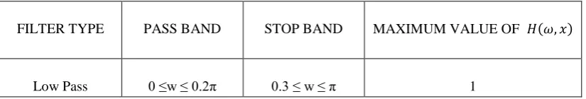
IV. SIMULATION RESULTS AND DISCUSSION

This section presents the work performed to implement the design of low pass digital FIR filter. The hybrid predator prey optimization algorithm has been applied to design low pass digital FIR filter, yielding optimal filter coefficients and compare it with PPO. Initially order of filter is taken as 20 which results in number of coefficients 21. The designing of low pass filter is done by setting 200 equally spaced samples within frequency range [0, π]. The prescribed design conditions for the low pass FIR digital filter are shown in Table 1.

Table 1: Design Conditions for Low Pass FIR Digital Filter

The algorithm is run 100 times and 200 iterations have been taken for obtaining best results at different orders. Initially population size is taken as 100, accelerating constants 𝒄𝟏and 𝒄𝟐 as 2.0, maximum weight as 0.4.

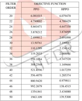
The performance of PPO compared with HPPO performance by varying order of filter from 20 to 50 for both algorithms and objective function has been observed.

Predator Prey Optimization

Order of filter has been varied from 20 to 50 and objective functions up to order 50 has been observed. Fig.1 shows the objective function variations with respect to order of filter. It shows that with the increase of filter order objective function increases continuously.

Figure 1: Order of Filter v/s Objective Function

The minimum value of objective function (2.699812) is observed at order 28 and after this the value of objective function starts increasing. So it is observed that optimum value of objective function seen at order 28 and at higher orders the value is deteriorated.

Hybrid Predator Prey Optimization

Predator prey optimization algorithm is hybridized using Hooke Jeeves Exploratory Move algorithm and results have been taken by varying order of filter. Order of filter has been varied from 20 to 50 and an objective function has been observed. Fig. 2 shows the objective function variations with respect to order of filter.

0 500 1000 1500 2000 2500

20 22 24 26 28 30 32 34 36 38 40 42 44 46 48 50

o

bje

ct

iv

e

fun

ct

io

n

order of the filter

FILTER TYPE PASS BAND STOP BAND MAXIMUM VALUE OF 𝐻(𝜔, 𝑥)

(8)

IJEDR1603082

505

Figure 2: Order of Filter v/s Objective Function

Table 2: Comparison of PPO and HPPO at Different Filter Orders

It is observed from Fig.1 and Fig.2 that in PPO, optimum objective function observed at order 28, but with the increase of filter order objective function increases continuously. So it is observed that optimum value of objective function seen at order 28 and at higher orders the value is deteriorated whereas in case of HPPO, the value of objective function decreases up to the order 44 and best objective function observed at order 44. After order 44, it starts increases and at order 48 again decreases and then after filter order 48 the value of objective function again increasing. So HPPO algorithm has the capability of giving enhanced performance than PPO algorithm at higher orders. HPPO proves itself superior in terms of objective function, magnitude errors, so HPPO chosen for further parameters tuning like 𝑐1, 𝑐2, IPOP.

0 20 40 60 80 100 120 140

20 22 24 26 28 30 32 34 36 38 40 42 44 46 48 50

o

bje

ct

iv

e

fun

ct

io

n

order of the filter

FILTER ORDER

OBJECTIVE FUNCTION

PPO HPPO

20 6.081015 6.079470

22 4.790002 4.789429

24 4.661671 4.647330

26 3.878212 3.876099

28 2.699812 2.691098

30 13.50761 2.199887

32 110.1289 2.154143

34 119.2033 2.088891

36 259.1034 1.347520

38 308.2568 1.169666

40 521.4396 1.017259

42 556.4070 1.285374

44 880.9420 0.979811

46 992.2679 138.4515

48 1354.841 3.434080

(9)

IJEDR1603082

506

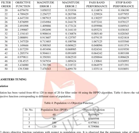
Table 3: Design of Low Pass digital FIR Filter for Different Orders using HPPO

FILTER ORDER

OBJECTIVE FUNCTION

MAGNITUDE ERROR 1

MAGNITUDE ERROR 2

PASS BAND PERFORMANCE

STOP BAND PERFORMANCE

20 6.079470 3.058332 0.331934 0.116874 0.106190

22 4.789429 2.256727 0.283706 1.229924 0.077955

24 4.647330 1.987915 0.283185 0.130257 0.070675

26 3.876099 2.034984 0.244178 0.073241 0.078127

28 2.691098 1.409886 0.173124 0.059986 0.049543

30 2.199887 1.092690 0.144110 0.055231 0.038183

32 2.154143 0.900616 0.136876 0.085140 0.020365

34 2.088891 0.913607 0.125707 0.079135 0.021818

36 1.347520 0.713403 0.100706 1.067125 0.035560

38 1.169666 0.500365 0.069623 0.048096 0.011574

40 1.017259 0.493496 0.068985 0.024341 0.019550

42 1.285374 0.504611 0.091609 0.064242 0.003188

44 0.979811 0.350301 0.062510 0.050044 0.006628

46 138.4515 9.547934 1.689424 1.130841 0.036993

48 3.434080 1.701396 0.218722 0.064979 0.071391

50 139.5300 7.470343 1.699170 1.035114 0.010691

PARAMETERS TUNING

Population

Population has been varied from 60 to 120 in steps of 20 for filter order 44 using the HPPO algorithm. Table 4 shows the values of objective function corresponding to different sizes of population.

Table 4: Population v/s Objective Function

Sr. No. Population Size (IPOP) Objective Function

1 60 0.659439

2 80 0.669598

3 100 0.979811

4 120 0.759086

Fig. 3 shows objective function variations with respect to population size. It is observed that the minimum value of objective function is observed at population size 60.

Figure 3: Population Size v/s Objective Function 0.5

0.6 0.7 0.8 0.9 1

60 80 100 120

o

bje

ct

iv

e

fun

ct

io

n

(10)

IJEDR1603082

507

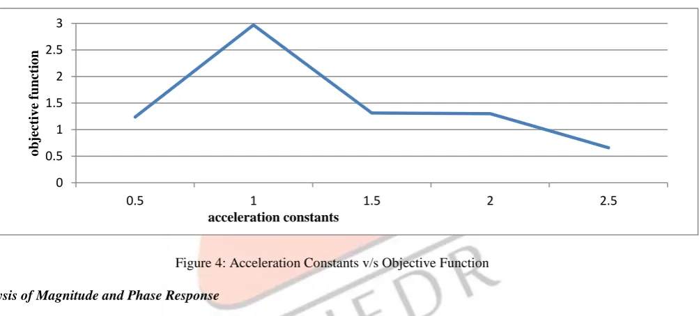
Acceleration Constants

Values of acceleration constants have been varied from 0.5 to 2.5 in steps of 0.5 for FIR filter design using HPPO. Table 5: Acceleration Constants v/s Objective Function

Sr. No.

Acceleration Constants (𝒄𝟏= 𝒄𝟐)

Objective Function

1 0.5 1.236719

2 1.0 2.968387

3 1.5 1.314512

4 2.0 1.301588

5 2.5 0.658774

Table 5 shows the variations of objective function with respect to acceleration constants 𝑐1 and 𝑐2. Minimum value of objective function observed at constants equal to 2.5. So order 44 with 𝑐1 and 𝑐2 equal to 2.5 has the minimum value of objective function. Fig. 4 shows the objective function variations with respect to acceleration constants.

Figure 4: Acceleration Constants v/s Objective Function Analysis of Magnitude and Phase Response

This section presents the simulation performed in MATLAB for the design of low pass FIR filter. The Fig.5 shows the graph for absolute magnitude response of order 44 for low pass digital FIR filter. Fig. 6 depicts the plot between absolute magnitude response in dB and normalized frequency for order 44 for the design of low pass FIR filter.

Figure 5: Plot of Magnitude Response v/s Normalized Frequency 0

0.5 1 1.5 2 2.5 3

0.5 1 1.5 2 2.5

o

bje

ct

iv

e

fun

ct

io

n

(11)

IJEDR1603082

508

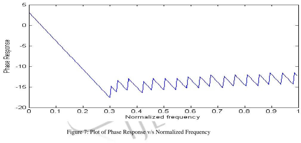
Figure 6: Plot of Magnitude Response in dBI v/s Normalized Frequency

Fig. 7 depicts the plot between phase response and normalized frequency for order 44 for the design of low pass FIR filter.

Figure 7: Plot of Phase Response v/s Normalized Frequency V. CONCLUSION

This paper proposes hybrid predator prey optimization method for the design of digital FIR filters. This algorithm enhances the capability to explore the search space locally as well globally to obtain the optimal filter design parameters. The right choice of parameters is very important to obtain great objective function. Order of filter varied from 20 to 50 and the order 44 gives the best value of objective function. Simulation results shows the better performance of proposed HPPO in terms of objective function, magnitude error and pass band and stop band performance. HPPO proves itself better for designing filters at higher orders and also the combination of global search and exploratory search optimization yields a powerful option for the design of FIR filters. HPPO method is effectively applied for the design of low pass, high pass, band pass and band stop digital FIR filters..

REFERENCES

[1] Emmanuel C. Ifeacher and Barrie W. Jervis, (2004), “Digital Signal Processing”, Pearson Publication, second edition. [2] Shahryar Rahnamayan, Hamid R. Tizhoosh and Magdy M. A. Salama, (2008), “Opposition Based Differential Evolution”,

IEEE Transaction on Evolutionary Computation, vol. 12, no. 1, pp. 64-79.

(12)

IJEDR1603082

509

[4] Abhijit Chandra and Sudipta Chattopadhyay, (2012), “Role of Mutation Strategies of Differential Evolution Algorithm in

Designing Hardware Efficient Multiplier-less Low-pass FIR Filter”, Journal of Multimedia, vol. 7, no. 5, pp. 353-363. [5] Sangeeta Mondal, Dishari Chakraborty, Rajib Kar, Durbadal Mandal and Sakti Prasad Ghoshal, (2012), “Novel Particle

Swarm Optimization for High Pass FIR Filter Design”, IEEE Symposium on Humanities, Science and Engineering Research, pp. 413-418.

[6] Balraj Singh, J.S. Dhillon and Y.S. Brar, (2013), “Predator Prey Optimization Method for the Design of IIR Filter”, Wseas Transactions on Signal Processing, vol. 9, no.2, pp. 51-62.

[7] Er. Mukesh Kumar, Rohit Patel, Er. Rohini Saxena and Saurabh Kumar, (2013), “Design of Band Pass Finite Impulse Response Filter Using Various Window Method”, International Journal of Engineering Research and Applications, vol. 3, no. 5, pp. 1057-1061.

[8] Balraj Singh, J.S. Dhillon, Y.S. Brar, (2013), “A Hybrid Differential Evolution Method for the Design of IIR Digital Filter”, International Journal on Signal & Image Processing, vol. 4, no. 1, pp. 1-12.

[9] Swati Chaudhary and Prof. Mamta M Sarde, (2014), “Review of Various Optimization Techniques for FIR Filter Design”, International Journal of Advanced Research in Electrical, Electronics and Instrumentation Engineering, vol. 3, no. 1, pp. 6566-6571.

[10] Amrik Singh and Narwant Singh Grewal, (2014), “Review on FIR Filter Designing by Implementations of Different Optimization Algorithms, International Journal of Advanced Information Science and Technology (IJAIST), vol. 31, no. 31, pp. 171-174.

[11] Pooja Yadav and Pooja Kumari, (2015), “FIR Filter Design”, International Journal of Innovative Research in Technology, vol. 1, no. 12, pp. 593-596.