de-Table 1: Web counts for each word.
printer print InterLaser ink TV Aquos Sharp
17000000 103000000 215 18900000 69100000 1760000000 2410000 186000000
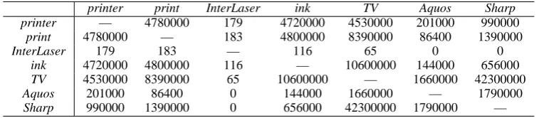
Table 2: Co-occurrence matrix by web counts.
printer print InterLaser ink TV Aquos Sharp printer — 4780000 179 4720000 4530000 201000 990000
print 4780000 — 183 4800000 8390000 86400 1390000
InterLaser 179 183 — 116 65 0 0
ink 4720000 4800000 116 — 10600000 144000 656000
TV 4530000 8390000 65 10600000 — 1660000 42300000
Aquos 201000 86400 0 144000 1660000 — 1790000
Sharp 990000 1390000 0 656000 42300000 1790000 —
structures of various networks are investigated in detail. For example, Motter (2002) targeted a conceptual network from a thesaurus and demon-strated its small-world structure. Recently, nu-merous works have identified communities (or densely-connected subgraphs) from large net-works (Newman, 2004; Girvan and Newman, 2002; Palla et al., 2005) as explained in the next section.
3 Word Clustering using Web Counts
3.1 Co-occurrence by a Search Engine
A typical word clustering task is described as fol-lows: given a set of words (nouns), cluster words into groups so that the similar words are in the same cluster 1. Let us take an example. As-sume a set of words is given: (printer),
(print), (InterLaser),
(ink), TV (TV), Aquos (Aquos), and Sharp (Sharp). Apparently, the first four words are lated to a printer, and the last three words are re-lated to a TV2. In this case, we would like to have two word groups: the first four and the last three.
We query a search engine3 to obtain word counts. Table 1 shows web counts for each word. Table 2 shows the web counts for pairs of words. For example, we submit a query printer AND In-terLaser to a search engine, and are directed to 179 documents. Thereby,nC2queries are necessary to
obtain the matrix if we havenwords. We call Ta-ble 2 a co-occurrence matrix.
We can calculate the pointwise mutual
informa-1
In this paper, we limit our scope to clustering nouns. We discuss the extension in Section 4.
2
InterLaser is a laser printer made by Epson Corp. Aquos is a liquid crystal TV made by Sharp Corp.
3Google (www.google.co.jp) is used in our study.
tion between wordw1andw2as
P M I(w1, w2) = log2
p(w1, w2)
p(w1)p(w2)
.
Probability p(w1) is estimated by fw1/N, where
fw1 represents the web count ofw1 andN
repre-sents the number of documents on the web. Prob-ability of co-occurrencep(w1, w2)is estimated by
fw1,w2/N wherefw1,w2 represents the web count
ofw1ANDw2.
The PMI values are shown in Table 3. We set N = 1010 according to the number of indexed
pages on Google. Some values are inconsistent with our intuition: Aquos is inferred to have high PMI to TV and Sharp, but also to printer. None of the words has high PMI with TV. These are be-cause the range of the word count is broad. Gen-erally, mutual information tends to provide a large value if either word is much rarer than the other.
Various statistical measures based on co-occurrence analysis have been proposed for es-timating term association: the DICE coefficient, Jaccard coefficient, chi-square test, and the log-likelihood ratio (Manning and Sch¨utze, 2002). In our algorithm, we use the chi-square (χ2) value in-stead of PMI. The chi-square value is calculated as follows: We denote the number of pages contain-ing bothw1andw2asa. We also denoteb,c,das
follows4.
w2 ¬w2
w1 a b
¬w1 c d
Thereby, the expected frequency of (w1, w2) is
(a+c)(a+b)/N. Eventually, chi-square is calcu-lated as follows (Manning and Sch¨utze, 2002).
Table 3: A matrix of pointwise mutual information.
printer print InterLaser ink TV Aquos Sharp printer — 4.771 8.936 7.199 0.598 5.616 1.647 print 4.771 — 6.369 4.624 -1.111 1.799 -0.463 InterLaser 8.936 6.369 — 8.157 0.781 −∞* −∞*
ink 7.199 4.624 8.157 — 1.672 4.983 0.900
TV 0.598 -1.111 0.781 1.672 — 1.969 0.370
Aquos 5.616 1.799 −∞*. 4.983 1.969 — 5.319 Sharp 1.647 -0.463 −∞* 0.900 0.370 5.319 —
* represents that the PMI is not available because the co-occurrence web count is zero, in which case we set−∞.
Table 4: A matrix of chi-square values.
printer print InterLaser ink TV Aquos Sharp
printer — 6880482.6 399.2 5689710.7 0.0* 0.0* 0.0*
print 6880482.6 — 277.8 3321184.6 176855.5 0.0* 0.0*
InterLaser 399.2 277.8 — 44.8 0.0* 0.0 0.0
ink 5689710.7 3321184.6 44.8 — 1419485.5 0.0* 0.0*
TV 0.0* 176855.5 0.0* 1419485.5 — 26803.2 70790877.6
Aquos 0.0* 0.0* 0.0 0.0* 26803.2 — 729357.7
Sharp 0.0* 0.0* 0.0 0.0* 70790877.6 729357.7 —
* represents that the observed co-occurrence frequency is below the expected value, in which case we set 0.0.
Figure 1: Examples of Newman clustering.
χ2(w1, w2)
= N×(a×d−b×c) 2
(a+b)×(a+c)×(b+d)×(c+d)
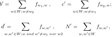
However,N is a huge number on the web and sometimes it is difficult to know exactly. There-fore we regard the co-occurrence matrix as a con-tingency table:
b0= ∑
w∈W;w6=w2
fw1,w, c
0= ∑
w∈W;w6=w1
fw2,w;
d0= ∑
w,w0∈W;w and w06=w1nor w2
fw,w0 , N0= ∑
w,w0∈W
fw,w0,
where W represents a given set of words. Then chi-square (within the word listW) is defined as
χ2W(w1, w2) =
N0×(a×d0−b0×c0)2
(a+b0)×(a+c0)×(b0+d0)×(c0+d0).
We should note that χ2W depends on a word set W. It calculates the relative strength of co-occurrences. Table 4 shows theχ2W values. Aquos has high values only with TV and Sharp as ex-pected.
3.2 Clustering on Co-occurrence Graph
Recently, a series of effective graph clustering methods has been advanced. Pioneering work that specifically emphasizes edge betweenness was done by Girvan and Newman (2002): we call the method as GN algorithm. Betweenness of an edge is the number of shortest paths between pairs of nodes that run along it. Figure 1 (i) shows that two “communities” (in Girvan’s term), i.e.{a,b,c} and {d,e,f,g}, which are connected by edge c-d. Edge c-d has high betweenness because numerous shortest paths (e.g., from a to d, from b to e,. . .) traverse the edge. The graph is likely to be sepa-rated into densely connected subgraphs if we cut the high betweenness edge.
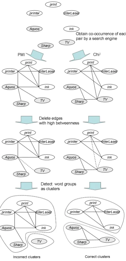
Figure 2: An illustration of graph-based word clustering.
this paper.
In Newman clustering, instead of explicitly cal-culating high-betweenness edges (which is com-putationally demanding), an objective function is defined as follows:
Q=∑
i (
eii− (
∑
j
eij )2)
(1)
We assume that we have separate clusters, and that eij is the fraction5 of edges in the network that
connect nodes in cluster i to those in cluster j. The termeiidenotes the fraction of edges within
the clusters. The term ∑jeij represents the
ex-pected fraction of edges within the cluster. If a
par-5We can calculatee
ijusing the number of edges between clusteriandjdivided by the number of all edges.
Figure 3: A word graph for 88 Japanese words.
ticular division gives no more within-community edges than would be expected by random chance, then we would obtainQ = 0. In practice, values greater than about 0.3 appear to indicate signifi-cant group structure (Newman, 2004).
Newman clustering is agglomerative (although we can intuitively understand that a graph with-out high betweenness edges is ultimately ob-tained). We repeatedly join clusters together in pairs, choosing at each step the joint that provides the greatest increase in Q. Currently, Newman clustering is one of the most efficient methods for graph-based clustering.
The illustration of our algorithm is shown in Fig. 2. First, we obtain web counts among a given set of words using a search engine. Then PMI or the chi-square values are calculated. If the value is above a certain threshold6, we invent an edge be-tween the two nodes. Then, we apply graph clus-tering and finally identify groups of words. This il-lustration shows that the chi-square measure yields the correct clusters.
The algorithm is described in Fig. 4. The pa-rameters are few: a thresholddthrefor a graph and,
optionally, the number of clustersnc. This enables
easy implementation of the algorithm. Figure 3 is a small network of 88 Japanese words obtained through 3828 search queries. We can see that some parts in the graph are densely connected.
4 Experimental Results
This section addresses evaluation. Two sets of word groups are used for the evaluation: one is derived from documents on a web directory; an-other is from WordNet. We first evaluate the
co-6In this example, 4.0 for PMI and 200 forχ2
Table 5: Examples of word groups from DMOZ-J.
category specific words to a category as a word group
(art) (gallery), (artwork), (theater), (saxophone), (verse), (live con-cert), (guitar), (performance), (ballet), (personal exhibition)
(recreation)
(raising), (poult), (hamster), (travel diary), (national park), (brewing), (boat race), (competition), (fishing pond)
(health) (illness), (patient), (myositis), (surgery), (dialysis), (steroid), (test), (medical ward), (collagen disease), (clinic)
Table 6: Examples of word groups from WordNet.
hypernym hyponyms as a word group
(gem) (amethyst), (aquamarine), (diamond),
(emer-ald), (moonstone), (peridot), (ruby), (sapphire),
(topaz), (tourmaline)
(academic field) (natural science), (mathematics), (agronomics), (architectonics), (geology), (psychology), (computer science), (cognitive science),
(sociology), (linguistics)
(drink) (milk), (alcohol), (cooling beverage), (carbonated beverage), (soda), (cocoa), (fruit juice), (coffee), (tea),
(mineral water)
Table 8: Precision of WordNet set. PMI Jaccard χ2 Mean 0.549 0.484 0.584
Min 0.473 0.415 0.498 Max 0.593 0.503 0.656 SD 0.037 0.027 0.048
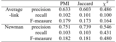
Table 9: Precision, recall and the F-measure for each clustering.
PMI Jaccard χ2
Average precision 0.633 0.603 0.486 -link recall 0.102 0.101 0.100 F-measure 0.179 0.173 0.164 Newman precision 0.751 0.739 0.546 recall 0.103 0.103 0.431 F-measure 0.182 0.181 0.480
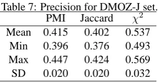
ing, which is often used in word clustering. A word co-occurrence graph is created using PMI, Jaccard, and chi-square measures. The threshold is determined so that the network den-sitydthreis 0.3. Then, we apply clustering to
ob-tain nine clusters; nc = 9. Finally, we compare
the resultant clusters with the correct categories. Clustering results for DMOZ-J sets are shown in Table 9. Newman clustering produces higher precision and recall. Especially, the combination of chi-square and Newman is the best in our ex-periments.
5 Discussion
In this paper, the scope of co-occurrence is document-wide. One reason is that major com-mercial search engines do not support a type of query w1 NEAR w2. Another reason is in (Terra
and Clarke, 2003) document-wide co-occurrences perform comparable to other Windows-based co-occurrences.
Many types of co-occurrence exist other than noun-noun. We limit our scope to noun-noun occurrences in this paper. Other types of co-occurrence such as verb-noun can be investigated in future studies. Also, co-occurrence for the second-order similarity can be sought. Because web documents are sometimes difficult to analyze, we keep our algorithm as simple as possible. An-alyzing semantic relations and applying distribu-tional clustering is another goal for future work.
A salient weak point of our algorithm is the number of necessary queries allowed to a search engine. For obtaining a graph ofnwords,O(n2) queries are required, which discourages us from undertaking large experiments. However some de-vices are possible: if we analyze the texts of the top retrieved pages by queryw, we can guess what words are likely to co-occur withw. This prepro-cessing seems promising at least in social network extraction: we can eliminate 85% of queries in the 500 nodes case while retaining more than 90% precision (Asada et al., 2005).
pro-G. Palla, I. Derenyi, I. Farkas, and T. Vicsek. 2005. Uncovering the overlapping community structure of
complex networks in nature and society. Nature,
435:814.
F. Pereira, N. Tishby, and L. Lee. 1993. Distributional clustering of English words. In Proc. ACL93, pages 183–190.
K. Tanaka-Ishii and H. Iwasaki. 1996. Clustering co-occurrence graph using transitivity. In Proc. 16th
In-ternational Conference on Computational Linguis-tics, pages 680–585.
E. Terra and C. Clarke. 2003. Frequency estimates
for statistical word similarity measures. In Proc.
HLT/NAACL 2003.
P. Turney. 2001. Mining the web for synonyms: PMI-IR versus LSA on TOEFL. In Proc. ECML-2001, pages 491–502.
P. Turney. 2002. Thumbs up or thumbs down? seman-tic orientation applied to unsupervised classification of reviews. In Proc. ACL’02, pages 417–424.
P. Turney. 2004. Word sense disambiguation by web
mining for word co-occurrence probabilities. In
Proc. SENSEVAL-3.
D. Widdows and B. Dorow. 2002. A graph model for unsupervised lexical acquisition. In Proc. COLING