Word-level Language Identification in Bi-lingual Code-switched Texts
Abstract
Code-switching is the practice of moving back and forth between two languages in spoken or written form of communication. In this paper, we address the problem of word-level language identification of code-switched sentences. Here, we primarily consider Hindi-English (Hinglish) code-switching, which is a popular phenomenon among urban Indian youth, though the approach is generic enough to be extended to other language pairs. Identifying word-level languages in code-switched texts is associated with two major challenges. Firstly, people often use non-standard English transliterated forms of Hindi words. Secondly, the transliterated Hindi words are often confused with English words having the same spelling. Most existing works tackle the problem of language identification using n-grams of characters. We propose some techniques to learn sequence of character(s) frequently substituted for character(s) in standard transliterated forms. We illustrate the superior performance of these techniques in identifying Hindi words corresponding to the given transliterated forms. We adopt a novel experimental model which considers the language and part-of-speech of adjoining words for word-level language identification. Our test results show that the proposed model significantly increases the accuracy over existing approaches. We achieved F1-score of 98.0% for recognizing Hindi words and 94.8% for recognizing English words.
1
Introduction
Code-switching is a popular linguistic phenomenon where the speaker alternates between two or more languages even within the same sentence. In countries like India, where there are
more than 20 widely used languages, code-switching is an even more pronounced feature, mostly among urban population (Thakur et al., 2007). Hindi and English are two popular ones among these languages, with millions of people communicating through them in pure forms or using a mixture of words from both the languages (code-switched), popularly known as ‘Hinglish’. Many multi-national brands use Hinglish taglines for promoting their products in India. For example, “Khushiyonki home delivery”1 is the tag line for Domino’s Pizza TM India. Hinglish is also used for casual communication among friends, for example, “Main temple ke pass hoon” meaning “I am near the temple”. There are plenty of research works focusing on analyzing texts used in popular forums, like online social groups, for applications like opinion mining, sentiment analysis, etc. However, machine analysis of Hinglish or any other code-switched text poses the following challenges.
• Inconsistent spelling usage: Despite the availability of the standards for transliteration (e.g., ITRANS 2 ) of Devanagari script to Roman script (the Hindi language is based on Devanagari script while the English language is based on Roman script), people tend to use many inconsistent spellings for the same word. For example, the most common English transliteration for the Hindi word
मैं
is mai, as observed from our data set. But people often use mein or main as alternatives.• Ambiguous word usage: The
transliterated word main, for the Hindi
1
http://www.dominos.co.in/blog/tag/khushiyon-ki-home-delivery/
2 ITRANS: http://www.aczoom.com/itrans/
Harsh Jhamtani
Suleep Kumar Bhogi
Vaskar Raychoudhury
Adobe systems
Samsung R&D institute
Dept. of Comp. Sc. & Engg.
Bangalore, India
Bangalore, India
IIT Roorkee, India
word
मैं
could be misinterpreted by a machine to be the English word.In order to address the afore-mentioned challenges and to enable automated analysis for code-switched languages, we need to identify the language of individual words. In case of transliterated Hindi words, we also need to find the authentic script. For example, in the sentence ‘Main temple ke pass hoon’ the word ‘main’ is a non-standard transliterated form for the Hindi word
मैं
and ‘pass’ refers to the Hindi wordपास
and not the English word.We propose some novel solutions to address the problem of word-level language identification in code-switched texts. Our major contributions can be summarized as below.
• We build a model to tackle the inconsistent spelling usage problem. The model learns the most common deviations from a standard transliteration scheme in English transliteration of Hindi words by identifying the erroneous character(s) that are frequently used in place of correct character(s) in standard transliterated forms.
• In addition to n-grams of characters, we use frequency of usage of a word in English and in Hindi languages as features for word-level language identification.
• We propose a technique using language and part-of-speech of neighboring words which, to the best of our knowledge, has not been applied before to solve this problem.
• We achieved F1-score of 98.0% for recognizing Hindi words and 94.8% for recognizing English words.
The rest of the paper is organized as follows. Section 2 describes the related work. Section 3 describes the data sets used. Section 4 describes the algorithms and features used. Section 5 describes the experiments conducted and their results.
2
Related Work
The socio-linguistic and grammatical aspects of code-switched texts have already been studied by many researchers. Ritchie and Bhatia (1996) and Kachru (1978) have discussed and examined different types of constraints on code-switching. Agnihotri (1998) discussed a number of examples of Hindi-English code-switching which do not comply with the constraints proposed in other literature. However, many of the constraints proposed for code switching, like the Free Morpheme Constraint (Sankoff and Poplack, 1981) and the Equivalence Constraint (Pfaff, 1979), are still widely applicable.
Automatic language identification research has focused on identifying both spoken languages as well as written texts. Language identification of speech has been studied by House and Neuburg (1977), where the authors assumed that the linguistic classes of a language are probabilistic functions of a Markov chain. Language identification of written texts has been studied at document-level as well as at word-level perspectives. Two major techniques adopted are n-gram (Cavnar and Trenkle, 1994) and dictionary-lookup (Řehůřek and Kolkus, 2009). Most of the existing research works on document-level language identification consider only mono-lingual documents (Hughes et al., 2006).
Word-level language identification in code-switched texts has received little attention so far. King and Abney (2013) have used weakly supervised methods based on n-grams of characters. However, their training data is limited to monolingual documents, which limits the capability to capture some patterns in code-switched texts. Nguyen and Dogruoz (2013) experimented with linear-chain CRFs to tackle the problem. But their contextual features are limited to bigrams of words. Our approach is more general in the sense we consider the language and POS (Part-of-speech) of the neighbouring words. So our approach will work for bigrams of words not present in training data.
change rules (SCR) that model possible phonological variant of the word, along with 3-gram model for dialect identification at word-level.
Aswani and Gaizauskas (2010) proposed a bi-directional mapping from character(s) in the Devanagari script to character(s) in the Roman script for the purpose of transliteration. But they have manually come up with a limited number of mappings. Dasigi and Diab (2011) used string based similarity metrics and contextual string similarity to identify orthographic variants in Dialectal Arabic.
3
Data Sets
In this section, we describe the datasets used for our experimentation.
3.1 Data set 1: Hinglish sentences
We have a dataset of 500 Hinglish sentences containing a total of 3,287 words (CNERG3). Each word is labeled as Hindi (H) or English (E). Out of these, 2420 are labeled as Hindi words while the rest 867 are labeled as English words. Corresponding to each Hindi word, the authentic Devanagari script is also written. Some examples from this dataset are given below.
bangalore\E ke\H=के technical\E log\H=लोग We have another data set of 1000 sentences of social network chats. To avoid any bias, the data set was tagged manually by three people not associated with this work. The mean Cohen’s kappa coefficient of inter-annotator agreement between the sets of annotations was 0.852. There were few disagreements on the language of some named entities. An example from this dataset is given below.
Main\H=मैं main\E temple\E ke\H=के pass\H=पास hoon\H=ह�ँ.
Above two data sets were clubbed to form the
Data set 1.
3.2 Data set 2: Transliteration Pairs
The data set comprises of commonly used multiple transliterated forms of Hindi words. It contains 30,823 Hindi words (Roman script) followed by the corresponding word in Devanagari script (Gupta et al., 2012). Some examples from this dataset are given below.
3 http://cse.iitkgp.ac.in/resgrp/cnerg/
tera तेरा thera तेरा
teraa तेरा teraaa तेरा
3.3 Data set 3: Hindi word-frequency list It is a Hindi word frequency list which has 117,789 Hindi words (in Devanagari script) along with their frequency computed from a large corpus (Quasthoff et al., 2006). Some examples of this dataset are as below:
लेने 2226 के 2143862
Also we generated a list standard transliteration forms of all these words using ITRANS rules. This list will be referred to as Translated Hindi Dictionary.
3.4 Data set 4: English word-frequency list It is a standard dictionary of 207,824 English words along with their frequencies computed from a large news corpus.
4
Word-level Language Identification
Our model contains two classifiers. The Classifier 1 works by combining four independent features as shown in the functional diagram Fig. 1. These features do not take into account the context of the word.Classifier 1 Classifier 2 English
Score Modified
Edit Distance
Hindi Score N-grams Features
HINGLISH
Sentences P(E,w)
POS Tagger (English)
POS Tagger (Hindi)
POS-tagged HINGLISH Sentences
Identified Language of Words
Fig 1. Functional Diagram of our Approach
The Classifier 2 operates on the output of
Classifier 1 and the POS tagged Hinglish sentences. This classifier considers some contextual features which take into account the language and POS of neighboring words.
4.1 Using Word-level features : Classifier 1 Here, we describe the features used for Classifier 1. The classifier outputs the probability P with
which w is an English word, for each word w in a Hinglish sentence. If we call this probability P(E, w), then P(H, w) = 1- P(E, w), where P(H, w) is the probability with which w is a Hindi word.
4.1.1 Common Spelling Substitutions and String Similarity (Modified Edit Distance) This feature is used to address the inconsistent spelling usage problem discussed in the Introduction section. To solve this problem, for every word we try to find the most similar word in our Transliterated Hindi Dictionary using string similarity algorithms, like ‘Edit Distance’ (Wagner and Fischer, 1974).
However, we observed cases in code-switching texts where this algorithm does not produce the intended outcome. For example, for the Hindi word खुशबू, the possible transliterated forms are
khushboo and khushbu with the former being the standard one. With the Edit Distance algorithm applied over the two forms, we shall get a dissimilarity value of 2. The same algorithm applied over the strings khushbu and khushi (ख़ुशी), which refer to different Hindi words, also gives the same dissimilarity value. However, for all practical purposes, khushbu is much closer to khushboo than it is to khushi. It is an observed fact that people often tend to substitute, ‘u’ in place of ‘oo’ while writing transliterated forms. But the Edit Distance algorithm does not capture this fact. We call this type of substitutions as common spelling substitutions.
To overcome this problem, we have developed a ‘Modified Edit Distance’ (MED) algorithm (Fig. 2) which considers the common spelling substitutions. The idea is similar to Weighted Edit Distance (Kurtz, 1996), but in case of MED we automate the process of deciding the corresponding
weights. We have experimented with four different methods to learn common spelling substitutions
using the Transliteration Pairs data set. Here we present the working of the four methods.
Method 1
In this method, given the standard transliterated form w1of a word and a non-standard form w2 of the same word, we try to generate substitution pairs by first aligning the consonants. We add ‘;’ at start and end of each word to act as delimiters. ‘;’
is also to be considered as a consonant for the following procedure.
Consider a variable i varying from 1 to length of
w1. For a consonant c at position i of w1, we try to align it with a consonant at the smallest position j
of w2 such that:
• jth character of w2 is same as c.
• No character of w2, at a position greater than or equal to j, has already been aligned.
• |j-i|<=3
If it is not possible to align a consonant, then it is not aligned. We define a segment to be a sequence of characters delimited by two aligned consonants (delimiting consonants inclusive). The two words will contain same number of segments. We consider two corresponding segments as substitution pairs if they do not have identical sequence of letters.
e.g. w1=;tera; , w2=;teraa;
S1 = {;t, ter, ra;} S2 = {;t, ter, raa;}
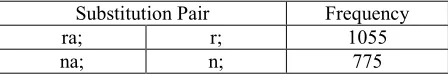
This generates a substitution pair (ra;, raa;). Some substitution pairs generated by this method are given in Table 1.
Substitution Pair Frequency
ra; r; 1055
na; n; 775
Table 1. Substitution pairs generated by Method 1
Method 2
For this method, the only difference with method 1 is in the way the segments are defined. We define a segment to be a sequence of characters delimited by two aligned consonants (delimiting consonants exclusive). We consider two corresponding segments as substitution pairs if they do not have identical sequence of letters. e.g. w1=;tera; , w2=;teraa;
S1 = {e, a}, S2 = {e, aa}
Substitution Pair Frequency
a aa 7764
a ha 872
Table 2. Substitution pairs generated by Method 2
Method 3
In this method, we do not include any delimiter at the beginning and end of the words. Rest of the working is same as in method 2.
Some substitution pairs generated by this method are given in Table 3.
Substitution Pair Frequency
a aa 8674
om on 1243
Table 3. Substitution pairs generated by Method 3
Method 4
In this method, we align the vowels also. Rest of the working is same as in Method 3.
For example, consider main (w1) and mein (w2) as two spelling variants of transliterated form of the Hindi word मैं. We first align ‘m’ of w1 with ‘m’ of w2, ‘i’ of w1 with ‘i’ of w2, and ‘n’ of w1
with ‘n’ of w2.
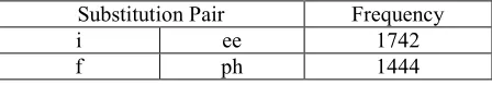
This generates the substitution pair (‘a’, ‘e’), i.e., ‘e’ has been used in place of ‘a’ interchangeably by the user. Some substitution pairs generated by this method are given in Table 4.
Substitution Pair Frequency
i ee 1742
f ph 1444
Table 4. Substitution pairs generated by Method 4
In all methods we keep some threshold thresh
for the frequency of substitution pairs. Substitution pairs occurring less than thresh are not further considered. The comparison of performance of MED based on these four methods will be discussed in the section 5.7.
Let subsList be the list of substitution pairs. Each entry s in subsList has attributes sx, sy, and sf,
where (sx, sy) is the substitution pair and sf is the corresponding frequency of occurrence.
Consider a substitution pair s which occurs with frequency sf in the training data. Then the cost of using the substitution is g(sf), i.e., a function of frequency sf. Here, g(f) = k / (log10(f)), where, k is a constant.
modifiedEditDistance (transliteration w1, transliteration w2, list of substitutions subsList)
N length of w1 M length of w2
initialize all elements of matrix dp[N][M] with 0 for i 1 to N:
for j 1 to M: if w1[i] == w2[j]: v1 dp[i-1][j-1] else:
v1 dp[i-1][j-1] + 1// substitution of a character v2 1 + dp[i-1][j] // deletion of a character v3 1 + dp[i][j-1] // insertion of a character v4 infinity
for s in subsList: p length of sx
q length of sy
if w1 [i-p+1 : i] = sx and w2[j-q+1 : j] =sy :
v4 min( v4 , g(sf) + dp[i-p][j-q] )
dp[i][j] min( v1, v2, v3, v4)
output: MED(w1,w2) = dp[N][M]
Fig 2. Pseudo code for Modified Edit Distance Algorithm
We have used logarithmic scaling as the frequencies of occurrences of the substitution pairs are very much skewed towards larger values. For every other insertion, deletion and substitution of a character, cost is 1 as is commonly used for Edit Distance. For each word w in test data, we try to match it against words in our Transliterated Hindi Dictionary. The word corresponding to the minimum cost and the minimum cost itself computed by the above algorithm are stored. The minimum cost so obtained for each word is
dissimilarityScore for that word. The algorithm for MED is shown in Fig.2.
4.1.2 Frequency of Occurrence in English and Hindi
‘main’, which can correspond to the Hindi word मैं or the English word. If we decide its language randomly, then the expected accuracy of identifying the correct language is 50%. If we know that main in English language is having higher usage frequency than the word मैं in Hindi language, then the probability of the test data word ‘main’ being an English word increases.
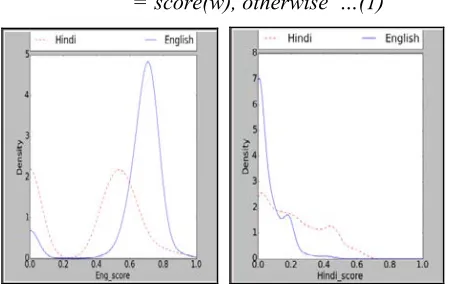
Using formula (1), we compute the value corresponding to this feature and we call it English score (eng_score). First, we use logarithmic scaling on frequencies of occurrences of English words to do away with its skewness towards large values. Then, we normalize the word frequency values with respect to the largest frequency observed.
M=max ( log( freq(q) ) )
∀ wordq ∈ Hindi Dictionary
For a given word w in the test data,
score(w) = log( freq(w))/M
eng_score(w) = 0, if w not in English Dictionary = score(w), otherwise …(1)
Fig 3. Density distribution plot for (a) English Score feature (b) Hindi Score feature
Similarly, we calculate the Hindi score (hin_score) using formula (2). However, first the MED algorithm is used to identify the closest matching Hindi word hw for a given word in the test data.
M=max ( log( freq(q) ) ) ∀ word q ∈ Hindi Dictionary
For a given word w in the test data,
score(w) = log( freq(hw))/M
hin_score(hw) = score(w) …(2)
Thus, we get English score and Hindi score for each word in the Dataset 1. The density
distributions of eng_score and hin_score are shown in Fig. 3(a) and Fig. 3(b) respectively.
4.1.3 Character N-grams
This follows the idea that, in Hinglish sentences some contiguous sequences of letters occur more frequently in words of one language as compared to the words of the other language. For example, bigram ‘es’ frequently occurs at the end of English words (like, roses, fries), often denoting plural morphological forms. We considered bigrams and trigrams of characters for the task of word-level language identification. We used the technique of Delta TF-IDF, which has been shown to be more effective in binary classification of class imbalanced data using unigrams, bigrams, and trigrams (Martineau et al., 2009)
For any term t (n-gram of characters) in word w, the Delta TF-IDF score V is computed using formula (3).
V(t,w) = n(t,w) * log2(Ht / Et) ----(3)
Where n (t, w) is the frequency count of term t
in word w. Ht and Et are the number of occurrences of term t in the English and Hindi dictionaries. Thus for every word w, we generate a set of feature values, with each n-gram t contributing one value.
4.2 Using Context Level Features: Classifier 2 All the previous features we have discussed focus on individual words of a code-switched sentence on a stand-alone basis, i.e., independent of the surrounding words or context. However, language usage of words in code-switched sentences may follow certain patterns, like words of a language are often surrounded by words of the same language (King and Abney, 2013). We tried to capture this context-dependence by considering the language and the POS of the surrounding words. For example, words on the two sides of conjunctions ‘and’, ‘aur (और)’, etc. are usually of same language as the conjunction.
possible POS usage, we consider the most frequent POS usage. For Hindi words, we used POS tagger by Reddy and Sharoff (2011). For each word w in the training data, we assign an identifier (id) X_P to it, where X can take values ‘E’ (for English) or ‘H’ (for Hindi), and P is the corresponding POS of the word. For example, if ‘car’ is an English noun (NN), then its id will be as E_NN.
We then count the number of occurrences of various bigrams of ids’ in the training data. We use these counts to calculate the conditional probability of an identifier to occur given the previous identifier e.g. P(id2|id1) is the probability that identifier id1 will be followed by identifier id2. For each word w, we have at most two possible candidate interpretations - Hindi word wH with POS as PwH, and English word wE with POS as
PwE. wH is found using MED algorithm and wE is found using English Dictionary lookup. Now w
refers to wE with probability P(E,w), and refers to
wH with probability P(H, w) e.g. if w is ‘main’, then wH is
मैं
and wE is the English word main. Now the identifier corresponding to w1H will be H_PRP asमैं
is a Hindi personal pronoun.Symbol Meaning
Sentence S A Hinglish sentence which is a sequence of words w1w2w3 … wN
Matrix
prob_pos[M][M] Conditional probability of the current word’s identifier (id) to be i, given that the identifier (id) of the previous word is j, as learnt from the training data.
Array
eng_prob[N] eng_prob[i] = P(E,w= Probability of the ii) th word in
sentence to be English, as provided by Classifier 1.
Array
hin_tag[N] hin_tag[i] = PwwiH iH = POS tag of
Array
eng_tag[N] eng_tag[i] = PwwiE iE = POS tag of
Integer M total number of identifiers possible Table 5. Notations and Symbols for classifier 2
Consider a Hinglish sentence S = w1w2w3…wn. A possible interpretation can be Sx = w1H w2H w3E … wNH. Now S has an interpretation given by Sx with probability P(S=Sx) given by:
P(S=Sx) = P(H,w1) * P(H,w2) * P(E,w3)..* P(H,wn) Now we define score (Sx) as follows:
score(Sx) = P(S=Sx) * P(id2|id1) * P(id3|id2)*... * P(idN|idN-1)
For a sentence S with N words, we can have a maximum of 2N such possibilities. Now calculating the maximum score over these possibilities has optimal sub-structures, which lets us use dynamic programming. Algorithm for Classifier 2 is presented in Fig.4. We built a similar model using trigrams of identifiers.
maxLikelihood (Sentence S, prob_pos[M][M], hindi_tag[N], eng_tag[N], eng_prob[N]): N length of s
Initialize all elements of dp [N+1][2] with 0 dp [0][0] 0.5
dp [0][1] 0.5 for i 1 to N:
/* dp [i][0] is the maximum score such that wi refers to
wiE when S[1,2,...i] have been considered */
/* dp [i][1] is the maximum score such that wi refers to
wiH when S[1,2,...i] have been considered */
prev_val dp [i-1][0] // 0 => english
v1 prev_val * eng_prob[i] * trans_prob[PwiE][Pwi-1E]
prev_val dp[i-1][1] // 1 => hindi
v2 prev_val *(1- eng_prob[i])*trans_prob[PwiE][Pw
i-1H]
dp [i][0] max(v1,v2)
// Similar procedure to calculate dp [i][1]
Fig. 4. Algorithm for Classifier 2 (using identifier bigram)
Consider following cases for the first three words of the sentence ‘Main main temple ke pass hoon’:
Case 1: Main (H_PRP) main (E_JJ) temple (E_NN)
Case 2: Main (E_JJ) main (E_JJ) temple (E_NN)
Case 3: Main (H_PRP) main (H_PRP) temple (E_NN)
Case 4: Main (E_JJ) main (H_PRP) temple (E_NN)
Case 1 is the correct case. The bigrams of identifiers corresponding to the case 1 i.e. H_PRP-E_JJ and H_PRP-E_JJ-E_NN occur much more frequently in the training data as compared to bigrams of other cases.
5
Experimentation and Results
5.1 Experiment 1: Presence in English Dictionary
In this experiment a word is classified as belonging to English class if it is present in English Dictionary otherwise the word is classified as belonging to Hindi class.
For this experiment, we sorted the words of the English Dictionary in decreasing order of the frequency of occurrences of words. Then we considered only the top K words for the experiment. The results for different values of K are shown in Table 6.
K HPR4 HRE HF1 EPR ERE EF1
100 0.74 0.98 0.84 0.31 0.02 0.04 500 0.76 0.96 0.85 0.59 0.15 0.24 1000 0.79 0.95 0.86 0.69 0.28 0.40 5000 0.85 0.93 0.89 0.75 0.55 0.64 10000 0.87 0.86 0.87 0.63 0.64 0.63 ALL 0.92 0.39 0.55 0.35 0.91 0.50
Table 6. Results of Experiment 1
We observed that with an increase in the number of words in the English dictionary, more English words will be correctly identified as ‘English’ words, resulting in increased recall values for the ‘English’ class (ERE). But at the same time more Hindi words would be incorrectly marked as English, resulting in decrease in HRE.
5.2 Experiment 2: King-Abney’s approach In this experiment we run the King’s (2013) n-grams and context level algorithms on our data set. The results are shown in Table 7.
HPR HRE HF1 EPR ERE EF1 Naïve
Bayes 0.66 0.83 0.74 0.39 0.20 0.27 HMM 0.75 0.91 0.83 0.59 0.29 0.39 CRF 0.76 0.96 0.85 0.76 0.28 0.41
Table 7. Results of Experiment 2
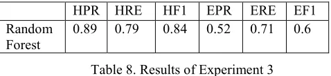
5.3 Experiment 3: Using Delta TF-IDF on n-grams of characters (Our Approach) In this experiment we used only one of our features for classification. We have used Delta TF_IDF
4HPR = Precision for Hindi class, HRE = Recall for the Hindi,
HF1 = f1 score for the Hindi class
EPR = Precision for English class, ERE = Recall for the English class, EF1 = f1 score for the English class
scores of n-grams of characters as features in our
Classifier 1. The results of experiment 3 are presented in Table 8. The best results are obtained using Random Forest with number of trees equal to 10.
HPR HRE HF1 EPR ERE EF1 Random
Forest 0.89 0.79 0.84 0.52 0.71 0.6 Table 8. Results of Experiment 3
5.4 Experiment 4: All word-level features (Classifier 1)
In this experiment we show the results produced by our Classifier 1 i.e., only using word-level features. Results of this experiment are presented in Table 9. We can see using other features, F1 scores have significantly increased.
HPR HRE HF1 EPR ERE EF1 Random
Forest 0.95 0.98 0.97 0.94 0.85 0.89 Table 9. Results of Experiment 4
Fig.5. ROC curve for Random Forest Classifier based on all word-level features
Thus best results came corresponding to Random Forest classifier, with number of trees = 10, and based on following word-level features:
• Delta TF-IDF on n-grams of characters
• eng_score
• hin_score
• dissimilarityScore
The corresponding ROC curve has been shown in Fig 5. The AUC (Area Under the curve) is 0.98.
5.5 Experiment 6: Classifier 2
As input to Classifier 2, we used POS tagged Hinglish sentences and the output of Classifier 1,
corresponding to the output from Experiment 4. We performed two experiments with Classifier 2 using bi-grams and tri-grams of identifiers. The results are shown in Table 10.
HPR HRE HF1 EPR ERE EF1 Identifier
bi-grams 0.974 0.969 0.972 0.920 0.934 0.926 Identifier
tri-grams 0.983 0.977 0.980 0.941 0.955 0.948
Table 10. Results of Experiment 6
The accuracy of Classifier 2 obtained on using identifier tri-grams is more than the accuracy obtained on using identifier bi-grams. This is probably because usage of trigrams captures the context more efficiently. Moreover the improvement offered by Classifier 2 over Classifier 1 is only little. This is mainly because of the already high accuracy values of Classifier 1.
We found that the percentage of named entities in the Dataset 1 is 8.59%. We observed that the percentage of named entities in the wrongly classified words is 23.2%.
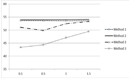
5.6 Experiment 7: Comparing four methods of creating substitution pairs
In this experiment we compare the results of previously described four methods to create substitution pairs. The results of this experiment is shown in Fig. 6. The K value which was defined in section 4.1.1 is varied to compare the results. It is observed that Method 2 gives best results among all methods discussed.
Fig 6. Graph showing comparison between four methods of creating substitution pairs
5.7 Performance of MED
To test the performance of MED algorithm in identifying correct Hindi words corresponding to
given transliterated forms, we compared it with the some other well-known string matching algorithms: Damerau-Levenshtein (49.38%), Levenshtein (47.48%), Jaro-Winkler (50%), Soundex (46.23%). The accuracy of MED is 54.1%.
For each Hindi word w in the Hinglish data-set, we try to match it against every word in our
Transliterated Hindi Dictionary. The word corresponding to the minimum cost is stored and later compared with the correct word. Fig.7 shows the results with a Hindi dictionary of size 117,789.
Fig 7. Performance of MED vs. other Algorithms
6
Conclusion
In this paper, we addressed the problem of word-level language identification in bilingual code-switched texts. We proposed a novel idea of utilizing the patterns in Hinglish sentences by considering the language and the POS of consecutive words. We proposed four different techniques to identify common spelling substitutions Our error analysis shows that a significant fraction of the errors made by the classifiers are actually named entities which are names of people or places, and can be considered either as Hindi or as English. In future, we would like to explore the changes of code-switching behavior from person to person. Also, we shall focus on other pairs of languages, like English-Bengali, English-Gujarati, etc. and also on word-level identification in multilingual code switched texts (i.e. having more than two languages).
7
References
Aravind K. Joshi. 1982. Processing of sentences with intra-sentential code-switching. In Proceedings of the 9th conference on Computational linguistics. Academia Praha, Volume 1: 145-150.
an utterance. I. Preliminary methodological considerations. The Journal of the Acoustical Society of America, 62: 708.
Baden Hughes, Timothu Baldwin, Steven Bird, Jeremy Nicholson, Andrew Mackinlay. 2006. Reconsidering language identification for written language resources. In Proc. International Conference on Language Resources and Evaluation: 485-488. Ben King, and Steven P. Abney. 2013. Labeling the
Languages of Words in mixed-language documents using weakly supervised methods. In Proceedings of the 2013 NAACL-HLT.
Braj B Kachru. 1978. Toward structuring code from the point of view of their usefulness in mixing: An Indian perspective. International Journal of the Sociology of Language, 16:28-46.
Carol W. Pfaff. 1979. Constraints on language mixing: intra-sentential code-switching and borrowing in Spanish/English, Language: 291-318.
David Sankoff, and Shana Poplack. 1981. A formal grammar for code ‐switching 1. Research on Language & Social Interaction, 14(1): 3-45.
Dong Nguyen, and A. Seza Dogruoz. 2013. Word level language identification in online multilingual communication. ACL 2013.
Fabian Pedregosa, Gael Varoquaux Alexandre Gramfort, Vincent Michel, Bertrand Thirion, Olivier Grisel, Mathieu Blondel, Peter Prettenhofer, Ron Weiss, Vincent Dubourg, Jake Vanderplas, Alexandre Passos, David Cournapeau, Matthieu Brucher, Matthieu Perrot, Édouard Duchesnay. 2011. Scikit-learn: Machine learning in Python. The Journal of Machine Learning Research, 12: 2825-2830.
Heba Elfardy, Mohamed Al-Badrashiny, and Mona Diab. 2013. Code Switch point detection in Arabic Natural Language Processing and Information Systems. Springer: 412-416.
Justin Martineau, Tim Finin, Anupam Joshi, and Shamit Patel. 2009. Improving binary classification on text problems using differential word features. In Proceedings of the 18th ACM CIKM.
Kanika Gupta, Monojit Choudhury, and Kalika Bali. 2012. Mining Hindi-English Transliteration Pairs from Online Hindi Lyrics, In Language Resources and Evaluation Conference: 2459-2465.
Kristina Toutanova, Dan Klein, Christopher D. Manning, and Yoram Singer. 2003. Feature-rich part-of-speech tagging with a cyclic dependency network.
In Proceedings of the NAACL-HLT, Volume 1: 173-180.
Niraj Aswani, and Robert J. Gaizauskas. 2010. English-Hindi Transliteration using Multiple Similarity Metrics. In Language Resources and Evaluation Conference.
Pradeep Dasigi, and Mona Diab. 2011. CODACT: Towards Identifying Orthographic Variants in Dialectal Arabic. In Proceedings of the 5th International Joint Conference on Natural Language Processing.
Radim Řehůřek, and Milan Kolkus. 2009. Language
identification on the web: Extending the dictionary method. In Computational Linguistics and Intelligent Text Processing.
Rama Kant Agnihotri. 1998. Mixed codes and their acceptability. Social psychological perspectives on second language learning: 191-215.
Robert A. Wagner, and Michael J. Fischer. 1974. The string-to-string correction problem. Journal of the Association for Computing Machinery (JACM), 21(1): 168-173.
Saroj Thakur, Kamlesh Dutta, and Aushima Thakur. 2007. Hinglish: Code switching, code mixing and indigenization in multilingual environment. Lingua Et Linguistica, 1.2 (2007): 109.
Siva Reddy, and Serge Sharoff. 2011. Cross language POS taggers (and other tools) for Indian languages: An experiment with Kannada using Telugu resources. Cross Lingual Information Access. Stefan Kurtz. 1996. Approximate string searching under
weighted edit distance. Proceedings of the 3rd South American Workshop on String Processing (WSP’96), Thamar Solorio, and Yang Liu. 2008. Learning to predict code-switching points. In Proceedings of EMNLP, 973-981.
Uwe Quasthoff, Matthias Richter, and Chris Biemann. 2006. Corpus portal for search in monolingual corpora. In Proceedings of the fifth international conference on language resources and evaluation: 1799-1802.
William B. Cavnar, and John M. Trenkle. 1994. N-gram-based text categorization. Ann Arbor M, 48113(2): 161-175.